Growth and Insecure Private Property of
Capital
Revised Version
Bertrand Crettez, Naila Hayek, Lisa Morhaim
∗†Abstract
This paper revisits Strulik’s model of growth with insecure property rights. In this model
different social groups devote some effort to control a share of the capital stock. We show
that a slight variation in the modeling of strategic interactions results in the coexistence
of savings and efforts to control a share of the capital stock. We also study the effects
of a change in the number of social groups on growth. We also show that an increase in
social fractionalization may lead to less effort devoted to control capital and to a higher
growth rate.
JEL Classification Numbers : C 73, D 02, D72, E 22, O 11, O 43.
Key Words : Dynamic Games, Insecure Private Property of Capital, Growth.
∗Universit´e Panth´eon-Assas, Paris II, CRED, [email protected].
†We thank two anonymous referees as well as the Editor, Georges Zaccour, for useful comments on a
1
Introduction
This paper addresses the effect of social composition in an economy where property
rights are unenforceable. It focuses on the case where individuals devote a part of their
productive time to appropriate a share of the available physical capital. In this setting
we ask the following question: How does social fractionalization affect investment and
predation activities?
Ogilvie and Carcus (2014) give an impressive overview of the link between private property
rights and growth from a historical perspective. To enhance growth, they argue, property
rights must be private, generalized (all agents must be able to access private property) and
secure. Security of property rights includes three aspects: security of ownership, security
of use, and security of transfers. These three types of security were gradually achieved
across history, at least in the economically developed part of the world, particularly in
Europe. These authors also argue that distributional conflicts are central in explaining
the development of property rights (and institutions in general) as well as the impact of
the latter on growth.
Gonzales (2012) offers an overview of the economics of insecure property rights and
economic backwardness. He focuses on the literature where, as in this paper, conflict uses
resources. This is in contrast with another strand in the literature on the economics of
insecure property rights (Benhabib and Rustichini, 1996, and Tornell and Lane, 1999).
This latter literature focuses on common-pool problems where agents try to redistribute
aggregate resources toward themselves, albeit without incurring direct conflict costs (see
Van Long, 2010, 4.6.2 and 7.2 for a presentation of this literature).
An important issue is the nature of the goods whose rights are insecure. In the literature
on economic growth with imperfect property rights it is often the case that agents are
assumed to have an insecure property right over their production. By contrast, it is at
the same time assumed that agents have complete property rights over consumption
and investment (capital) goods. To put it differently, while individuals only control a
certain share of their output, theuses of this share are secure. A notable exception in the
literature is Strulik (2008). Strulik considers an infinite horizon differential game where
the property of capital is insecure. In this setting, agents (or rather groups of agents)
hand, agents have complete property rights over their individual production (and the
consumption good). Thus, in Strulik’s model, capital can be thought off as a common
good. The access to this good, however, is not free, but depends on the issue of a conflict.1
Among Strulik’s findings two deserve to be singled out. First, Strulik shows that conflict
and growth cannot coexist in a symmetric society (where all groups have the same size).
That is, it is impossible that all groups both invest and try to control a share of capital. As
for the second result, Strulik shows that an increase in social fractionalization negatively
affects growth.
Strulik’s approach is interesting in the light of the recent literature of economic development
and social conflict (namely within-country conflicts), a survey of which can be found in
Ray and Esteban (2017). These authors argue that conflicts occur across economically
similar, rather than different, groups, and over the direct use of resources. As they put
it (p. 267): “Because the conflict is over the direct use of a resource, the groups are
often remarkably similar in their economic characteristics...The gains from conflict are
immediate: the losing group can be excluded from the sector in which it directly competes
with the winners.”2
This paper revisits Strulik’s model of growth with insecure property rights. Our framework
differs from Strulik’s in four respects.
First we use a sequential instead of a differential version of the model. This enables us to simplify the study of the feedback-Nash equilibria. Second, we rely on a standard neo-classical production technology, whereas Strulik sup-poses that the production function is the product of capital and labor. This assumption allows him to easily obtain perpetual growth. On the other hand, Strulik’s specification implies increasing returns to scale at the level of a social group as opposed to society as a whole, which is not obvious.3 Third, and more importantly, we assume that people take other agents’ savings rule as given.
1In the literature on the depletion of common resources, it is possible to accumulate some privately
and safely held capital, but there is no costly competition to access the resources.
2They also write that: “ethnicity is possibly a marker for organizing similar individuals along opposing
lines.”
3We do not focus on perpetual growth. We could obtain endogenous growth by assuming
By contrast, in Strulik’s setting, people take other agents’ consumption rules as given. This difference in the modeling of strategic interactions enables us to show that conflict can coexist with growth in a symmetric society.4 This
result is of interest since it is empirically established that the coexistence of conflict and growth can occur (Polachek and Sevastianova, 2012). Fourth, we also investigate a larger class of conflict technologies. We show that there are conflict technologies, more precisely, contest success functions, such that the predation effort is a decreasing function of social fractionalization. While it is certainly true that the predation effort is empirically an increasing function of social fractionalization (in this respect Strulik’s second result is supported by the facts), our theoretical finding shows that a change in the conflict technol-ogy can be welfare improving. This is interesting as it seems easier to change the conflict technology than the whole property rights system.
The remaining part of the paper unfolds as follows. In the next section we lay out the
model and the definition of the dynamic equilibrium used in the paper. We establish
the existence of an interior feedback Nash equilibrium in section 3. Section 4 shows that
the difference between this result and Strulik’s is due to a difference in the modeling of
strategic interaction. Section 5 addresses the effects of social fragmentation (namely, how
the number of social groups affects the equilibrium decisions). We notably present a case
where more fragmentation is not detrimental to growth. We provide some concluding
remarks in section 6.
2
Model and Definitions
2.1
Model
There are n identical agents (each representing a group of individuals), superscribed by i,
planning their decisions over an infinite discrete time horizon.
As there is no secure private ownership of capital, at each date t, agents compete for a
4Strulik shows that conflict and growth can coexist in an economy populated by two groups ofunequal
share of the total capital stock kt. The dynamics of this total capital stock is given by
kt+1 =
n
X
i=1
eit+ (1−δ)kt, (1)
where ei
t is the savings of agent i at date t, and δ is the capital depreciation rate.
To access the stock of capital, agents must spend some resources. Specifically, we assume
that agents devote a part τti of their productive time (τti ∈[0,1]), dubbed predation time,
to get some capital. The share of the aggregate capital stock accruing to agentiis given by
a function φ(τti,τt−i), φ: [0,1]n→[0,1], where τt−i stands for the vector of the predation efforts of all agents except i.5 We shall specifically assume that
φ(τti,τt−i) = g(τ i t)
g(τi
t) +Pj6=ig(τ j t)
, (2)
where g : [0,1]→R+
∗ is increasing.
Agent i’s resource constraint then reads
fÄφ(τti,τt−i)kt,1−τti
ä
=eit+cit, (3)
where f :R+×[0,1]→R+ is the production function, and cit is the value of consumption
at datet.
We assume that the issues of the agents’ interactions are given by the Nash equilibria of
dynamic games where each agent i solves the next problem
max
(ei t,τti)
+∞
X
t=0 βtU
Ç
fÄφ(τti,τt−i)kt,1−τti
ä
−eit
å
. (4)
where the utility function U is an increasing function defined on either R+ or R∗+.
2.2
Definitions
To further the analysis of the interaction of the n agents we suppose that each player i
uses stationary Markovian strategies. That is, we assume that the decisions (τti, eit) made
by agent i at date t are given by a function Si of the capital stock k
t. We let S be the vector of these individual decisions (itsi-th coordinate being equal to Si).
Definition 1. We denote by Πi(¯t, k
¯
t,S) the value of agent i’s objective at date t¯, when
the value of the capital stock at this date is k¯t, and when agents’ strategies are given by S.
5Physical feasibility implies thatPn
Namely:
Πi(¯t, kt¯,S) = +∞
X
t=¯t
βtU
Ç
fÄφ(τti,τt−i)kt,1−τti
ä
−eit
å
(5)
when for each i, and at each date t, (τi
t, eit) = Si(kt) and kt+1 =Pni=1eit+ (1−δ)kt.
Definition 2. A feedback Nash equilibrium is a set of functions Si : R+ →[0,1]×R+,
one for each agent i, which are such that for each date ¯t, for each capital stock k¯t at
this date and for each player i, Πi¯t, k¯t, Si,S−i
≥ Πit, k¯ ¯t, S,S−i
, for all functions
S :R+→[0,1]×R+ and with kt+1 =Pni=1eit+ (1−δ)kt.
A symmetric feedback Nash equilibrium is a feedback Nash equilibrium in which Si =S
for all i.
To find a feedback Nash equilibrium, we shall look for Markovian strategies Si which are
such that Bellman equation is satisfied for all k and for all agents i
Vi(k;S−i) = U
Ç
fÄφ(τi,τ−i)k,1−τiä−ei
å
+βVi
k0;S−i, (6)
= max τi,ei
®
U
Ç
fÄφ(τi,τ−i)k,1−τiä−ei
å
+βVik0;S−i ´
(7)
where: (τi, ei) =Si(k), k0 =ei+P
j6=iej. We obtain a feedback Nash equilibrium when
β¯tVi(k;S−i) = Πi(¯t, k,S), for all k and for all ¯t.
The problem at hand is unfortunately a non-convex one, notably because of the term φ in
the production function. To address this non-convexity we shall focus on the specific case
where U(c) = lnc, f(k, l) = (k)α(l)1−α, 0< α <1 andδ = 1. However, we shall leave g(.)
unspecified in most of the analysis.6 7
6We thank a referee for noticing that Strulik’s production function, namelyf(k, l) =klis
not a special case of our production function when α= 1. To obtain Strulik’s specification from a Cobb-Douglas function we could set: yt= (Atkt)α(Btlt)1−α where, following Frankel
(1962) and Romer (1986), At =lt, and Bt=kt. Generally, it is assumed that the decision
maker is unaware of the specifications of At and Bt, except if he is a social planner. That
a social group behaves as a social planner is not strictly impossible, but this is probably a strong assumption.
7In appendix A we show that under our specific assumptions the values of the agents’
3
A Feedback Nash Equilibrium
Since U is an increasing function, a glance at equation (7) shows that at each date the
shares of aggregate capital accruing to the different agents are the Nash equilibria of the
static game where each agent solves
max τi f
Ç
φ(τi,τ−i)k,1−τi
å
, (8)
k being given.
Under the assumption that f is Cobb-Douglas, we can see immediately to see that a
Nash equilibrium of the predation game does not depend on k. This leads us to study a
feedback Nash equilibrium by first considering the equilibria of the predation game, and
second the dynamic savings game.
3.1
The Predation Game
A symmetric Nash equilibrium of the predation game is defined as follows.
Definition 3. τ∗ in [0,1] is a symmetric Nash equilibrium for the predation game if τ∗
belongs to arg maxτ∈[0,1]F(τ, τ∗), where the function F : [0,1]2 →R is defined by
F(τ, τ0) =
Ç
g(τ)
g(τ) + (n−1)g(τ0) åα
(1−τ)1−α. (9)
The following assumption will be useful to prove the existence of an interior symmetric
Nash equilibrium.
Assumption G. g : [0,1]→Ris increasing, concave, differentiable on ]0,1[ and satisfies
g(0)>0, gg0(0)(0) > n n−1
1−α α .
To prove the existence of a symmetric Nash equilibrium of the predation game we establish
two technical Lemmata.
Lemma 1. Assume that G holds. Then for any τ0 ∈[0,1], the function τ 7→F(τ, τ0) is strictly quasiconcave on [0,1].
Proof. We can check that the function τ 7→ g(τ)+(gn(−τ)1)g(τ0) is strictly concave and thus
τ 7→αlng(τ)+(gn(−τ)1)g(τ0)+ (1−α) ln(1−τ) is strictly concave. It follows thatτ 7→F(τ, τ
0) is
Lemma 2. Assume that G holds. For all τ0 in [0,1], we have
lim τ→0+F
0
1(τ, τ
0
)>0, (10)
lim τ→1−F
0
1(τ, τ
0
)<0. (11)
Proof. After some computations we obtain that
F10(τ, τ0) =
Ç
g(τ)
g(τ) + (n−1)g(τ0) åαÇ
α(n−1)g
0(τ)g(τ0)(1−τ)1−α
g(τ) [g(τ) + (n−1)g(τ0)] −(1−α)(1−τ) −α
å
.
(12)
Notice that [g(τ()+(n−n1)−g1)(τg0)(τ0)] is an increasing function ofτ
0. So (n−1)g(τ0)
[g(τ)+(n−1)g(τ0)] >
(n−1)g(0) [g(τ)+(n−1)g(0)]
The result follows (inequation (10) results from the assumption made on g).
Using the two above Lemmata, we have
Proposition 1. Assume that G holds. Then there exists a unique interior symmetric Nash equilibrium.
Proof.
Step 1 (Existence).
As F is continuous, for anyτ0 ∈[0,1], the problem
max τ∈[0,1]F(τ, τ
0
) (13)
has a solution. Moreover, it is unique since by Lemma 1 F is strictly quasiconcave.
Let m : [0,1] → [0,1] be the function defined by m(τ0) = arg maxτ∈[0,1]F(τ, τ0), for
any τ0 ∈ [0,1]. By Berge’s Maximum Theorem (see the version given in Theorem 3.6,
Lucas, Stokey with Prescott, 1989), m is continuous on [0,1]. By Brouwer’s theorem,
m: [0,1]→[0,1] has a fixed-point.
Step 2 (Interiority) It is immediate by Lemma 2.
Step 3 (Uniqueness). Any interior symmetric Nash equilibrium satisfies the condition
F10(τ, τ) = 0, which can be expressed as
α(n−1)
n
g0(τ)
g(τ) = 1−α
1−τ. (14)
Under our assumptions on g, the left-hand side decreases with τ, whereas the right-hand
A Remark. AssumptionG, and in particular, the concavity assumption regarding g, is not necessary for the existence of an interior equilibrium. For instance, there may be a
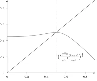
symmetric equilibrium when g(τ) =e1−στ, σ >0. The figure 1 below represents the graph
of an agent’s objective when : n = 2, σ = 4, α = 1/5. There is an interior symmetric
Nash equilibrium at τ = 1/2.
0 0.2 0.4 0.6 0.8
0 0.2 0.4 0.6 0.8
e
4
1−τ(1−τ)4
e
4 1−τ+e8
15Figure 1: An interior equilibrium of the predation game wheng(τ) =e1−στ.
3.2
Equilibrium savings
We turn next to the study of the savings game. We have
Proposition 2. Assume that there exists a symmetric interior equilibrium τ for the static predation game. Then there exists a symmetric feedback Nash equilibrium where
S(kt) = (τ,n(1−αβαβ)+αβ(1−τ)1−α
Äk
t
n
äα
).
Proof.
• First step
We look for a candidate value function. To do this, we conjecture that the policy function
That is, we conjecture that
eit(kt) =e(kt) =θ
Äkt
n
äα
(1−τ)1−α, (15)
where θ ∈[0,1]. In the above expression we have used the assumption that the predation
game has an interior symmetric equilibrium, so thatφ(τ, τ) = 1/n. Under our assumption
on the policy function, we have: ct= (1−θ)
Äk
t
n
äα
(1−τ)1−α,and
lnct= ln
ñ
(1−θ)(1−τ)
1−α
nα
ô
+αlnkt. (16)
Since
kt+1 =
X
i
eit =ne, (17)
=θ[(1−τ)n]1−αÄkt
äα
, (18)
we have
lnkt+1 = ln
î
θ[(1−τ)n]1−αó+αlnkt. (19)
The solution of this first-order difference equation writes
lnkt=αt(lnk0−lnk∞) + lnk∞, (20)
where
lnk∞ =
ln [θ[(1−τ)n]1−α]
1−α . (21)
Using the expressions of lnct and lnkt we can show that
∞
X
t=0
βtU(ct) = 1 1−β
Ç
ln
ñ
(1−θ)(1−τ)1−α
nα
ôå
+ αβ(1−α)
(1−β)(1−αβ)lnk∞+
α
1−αβ lnk0, (22)
≡ V(k0;θ). (23)
• Second step.
Now we shall look for a value of θ. We conjecture that the value function will have the
same expression as V(kt;θ). For the Bellman equation to be satisfied, we must find a
value ofθ such that:
V(kt;θ) = max ei
t,τi
¶
lnîÄφ(τi, τ)kt
äα
(1−τi)1−α−etió+βV(kt+1;θ)
©
where kt+1 =eit+ (n−1)θ
Äk
t
n
äα
(1−τ)1−α (all agents buti use the same saving function).
Concentrating on the right-hand side of the Bellman equation, we consider the following
problem
max ei
t,τi
®
lnîÄφ(τi, τ)kt
äα
(1−τi)1−α−eitó+β
®
1 1−β ln
ñ
(1−θ)(1−τ)
1−α
nα
ô
+ 1−α
(1−β)(1−αβ)αlnk∞+
α
1−αβ ln
ñ
eit+ (n−1)θ(1−τ)1−αÄkt
n
äα ô´
. (25)
Assume that there is an interior solution. Then this solution satisfies:
−1
Ä
φ(τi, τ)k t
äα
(1−τi)1−α−e t
+ αβ
1−αβ
1
et+ (n−1)θ(1−τ)1−α
Äk
t
n
äα = 0. (26)
By assumption there exists a positive symmetric equilibrium for the predation game.
Thus τi =τ and φ(τ, τ) = 1/n. As in equilibrium eit =θ(1−τ)1−αÄknäα we obtain from
equation (26) that
θ∗ = αβ
n(1−αβ) +αβ. (27)
• Third step
We now check that the two sides of the Bellman equation are the same.
To do this observe that the right-hand side of the Bellman equation is given by:
max ei t ® ln ñ
(1−τ)1−αÄkt
n
äα
−eit
ô
+βV(kt+1;θ∗)
´
= ln
ñ
(1−θ∗)(1−τ)
1−α
nα
ô
+αlnkt
+ β
1−βln
ñ
(1−θ∗)(1−τ)
1−α
nα
ô
+αβlnk∞
(1−α) (1−β)(1−αβ)
+ αβ
1−αβ
Ä
(1−α) lnk∞+αlnkt
ä
,
(28)
with
lnk∞=
ln [θ∗[(1−τ)n]1−α]
1−α . (29)
After some computations, we obtain
max ei t ® ln ñ
(1−τ)1−αÄkt
n
äα
−eit
ô
+βV(kt+1;θ∗)
´
= 1
1−β ln
ñ
(1−θ∗)(1−τ)1−αÄkt
n
äα ô
+ αβ(1−α)
(1−β)(1−αβ)lnk∞
+ α
which is indeed equal to V(kt;θ∗).
• Fourth step
We still need to show that the above solution of the Bellman equationis the value function
V(k0) where for all k0
V(k0) = sup (ct,τt,kt)t
∞
X
t=0
βtlnct, (31)
and
ct≤
Ç
g(τt)
g(τt) + (n−1)g(τ)kt
åα
(1−τt)1−α, (32)
kt+1 = (n−1)ψkαt +
Ç
g(τt)
g(τt) + (n−1)g(τ)
kt
åα
(1−τt)1−α−ct, (33)
with ψ = (1/n)α(1−τ)1−α.8
Now, consider the candidate value function:
V(k;θ∗) = 1 1−βln
ñ
(1−θ∗)(1−τ)1−αÄk
n
äα ô
+ αβ(1−α)
(1−β)(1−αβ)lnk∞+
α
1−αβ lnk,
(34)
Let us establish that for a feasible path (ct, τt, kt)t such that limT→+∞PTt=0βtlnct>−∞
we have limt→+∞βtV(kt;θ∗) = 0. First, using the sequence (¯kt)t introduced in the
appendix, we can show that lim supt→+∞βtV(k
t;θ∗)≤0.
Now, since V(.;θ∗) satisfies the Bellman equation, we have for allT > 0
−∞<
∞
X
t=0
βtlnct≤ T
X
t=0
βtlnct+βT+1V(kT+1;θ∗). (35)
Hence,
∞
X
t=0
βtlnct− T
X
t=0
βtlnct≤βT+1V(kT+1;θ∗). (36)
As
0 = lim T→+∞
"∞ X
t=0
βtlnct− T
X
t=0
βtlnct
#
≤lim inf T→+∞β
T+1V(k
T+1;θ∗), (37)
the result follows. Now let us show that V(k0;θ∗) =V(k0) for all non-negative k0. This is
also true for k0 = 0. Let us then assume that k0 > 0. Since V(.;θ∗) is continuous and
satisfies the Bellman equation, there exists a feasible path (ct, τt, kt)t such that
V(k0;θ∗) =
T
X
t=0
βtlnct+βT+1V(kT+1;θ∗), (38a)
≤ +∞
X
t=0
βtlnct+ lim sup T→∞
βT+1V(kT+1;θ∗), (38b)
≤ +∞
X
t=0
βtlnct, (38c)
≤V(k0). (38d)
As k0 >0, for each feasible sequence from k0, we have
V(k0;θ∗)≥
T
X
t=0
βtlnct+βT+1V(kT+1;θ∗). (39)
If we let T go to infinity, we obtain:
V(k0;θ∗)≥
∞
X
t=0
βtlnct+ lim T→∞β
T+1V
(kT+1;θ∗), (40)
=
∞
X
t=0
βtlnct. (41)
Thus
V(k0;θ∗)≥V(k0). (42)
We conclude that V(.;θ∗) = V(.).
We have therefore shown that there is an interior feedback Nash equilibrium in which
each agent both saves and devotes a part of the productive time to appropriating the
be seen by inspecting equation (25). The termei
t+(n−1)θ(1−τ)1
−αÄk
t
n
äα
is equal to kt+1 (and thus appears in the expression V(kt+1;θ) in the right-hand side of
the Bellman equation). The part (n−1)θ(1−τ)1−αÄk
t
n
äα
in the expression of
kt+1 represents the equilibrium value of other agents’ savings. In equilibrium,
the share θ of production devoted to savings is low so that the value of ei t
maximizing the right-hand side of the Bellman equation is non nil.
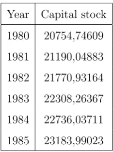
As we have already mentioned, in Strulik’s model, conflict and growth cannot coexist in a symmetric society. Before addressing the reason underlying the difference between this result and ours, we briefly consider the empirical sup-port of the coexistence of conflict and growth. In that connection, a study by Polachek and Sevastianova (2012) shows that growth can happen with intra-national conflicts.9 As the authors put it: “...neither international wars nor
civil wars necessarily reduce per capita income, and in fact can temporarily raise it.” (pp. 9). For instance, growth occurred for Uganda during the period 1981-1985, where according to Polachek and Sevastianova a domestic intrastate war took place. Of course, this growth in per capita income could have happened without any investment. But if we look at the capital stock of Uganda, we can see that this stock increased every year between 1980 and 1985.10 The values of the capital stock are displayed in figure 2.
9A working paper is also available at:
https://www.iza.org/publications/dp/4762/does- conflict-disrupt-growth-evidence-of-the-relationship-between-political-instability-and-national-economic-performance.
10The data are available in Feenstra, Robert C., Robert Inklaar and Marcel P. Timmer
(2015), “The Next Generation of the Penn World Table”,American Economic Review, 105 (10), 3150-3182, available for download at www.ggdc.net/pwt The capital stock is evaluated
Year Capital stock
1980 20754,74609
1981 21190,04883
1982 21770,93164
1983 22308,26367
1984 22736,03711
1985 23183,99023
Figure 2: Capital stock in Uganda 1980-1985
In the next section we emphasize the difference between our setting and Strulik’s which
explains the difference in our results.
4
Comparison with Strulik’s Approach
Recall that the problem faced by each agent is
max
+∞
X
t=0
βtU(cit) (43)
such that
f
Ç
g(τti)
Pn
j=1g(τ
j t)
kt,1−τti
å
=cit+eit, (44)
kt+1 = (1−δ)kt+ n
X
j=1
ejt, (45)
eit≥0, (46)
cit≥0, (47)
0≤τti ≤1. (48)
So far we have specifically focused on the following problem
max
+∞
X
t=0 βtU
Ñ
f
Ç
g(τti)
Pn
j=1g(τ
j t)
kt,1−τti
å
−eit
é
such that
kt+1 = (1−δ)kt+ n
X
j=1
ejt, (50)
0≤eit≤f
Ç
g(τi t)
Pn
j=1g(τ
j t)
kt,1−τti
å
, (51)
0≤τti ≤1. (52)
Strulik’s approach is different.11 Instead of havingk
t+1 = (1−δ)kt+Pni=1eitand assuming that all the effort but ei
t are given, Strulik substitutes
f
Ç
g(τtj)
Pn
h=1g(τth)
kt,1−τtj
å
−cjt
for ejt in equation (50). This implies in particular that τi
t will affect every individual production through the terms g(τ
j t)
Pn
h=1g(τth).
Strulik indeed considers the following problem
max
+∞
X
t=0
βtU(cit) (53)
such that
kt+1 = (1−δ)kt+ n X j=1 ( f Ç
g(τtj)
Pn
h=1g(τth)
kt,1−τtj
å
−cjt
)
, (54)
0≤cit≤f
Ç
g(τi t)
Pn
j=1g(τ
j t)
kt,1−τti
å
, (55)
0≤τti ≤1. (56)
Notice that in this approach social groups are assumed to take into account the fact that an increase in their predation effort decreases ceteris paribus
the shares of the capital stock held by of all the other people. In particular, a social group takes into account the fact that an increase in its predation effort will lead to a decrease in the savings of the other groups (through a decrease in the value of their production, their consumption decisions being assumed to be unaffected). This may be considered as a rather strong assumption.
11Recall that Strulik uses a continuous time setting. We translate his modeling assumptions in a
Proposition 3 (Strulik). Assume that U0(c)>0 andf20 >0. Then there is no symmetric interior equilibrium in Strulik’s approach.
Proof. If (cit, τti) is interior i.e. 0< cit< f
Ç
g(τi t)
Pn j=1g(τ
j t)
kt,1−τti
å
and 0< τti <1, then by
Theorem 2.2 12 in Blot and Hayek (2014), the necessary conditions of optimality include
the following ones13
U0(cit) =βqti+1 (57)
0 =βqti+1
Ñ
g0(τi t)g(τti)
ÄPn
j=1g(τ
j t)
äf
i
1kt−f2i−
n X h=1
g0(τi t)g(τth)
ÄPn
j=1g(τ
j t)
ä2f
h
1kt
é (58) (59)
=βqti+1
Ç
(n−1)g0(τ)
n2g(τ) f
i
1kt−f2i−(n−1)
®
g0(τ)
n2g(τ)f
i
1kt
´å
. (60)
The last equation can be rewritten as follows
0 =−βqi t+1f
i
2. (61)
It follows that: qti+1 = 0 sincef2 >0. But then we get U0(cit) = 0, which is impossible by
assumption.
5
Effects of Social Fractionalization
In our model, society is clustered in n symmetric groups (whose size is equal to one). An
increase inn leads to an increase in the value of the fractionalization index 1−(1/n).14
12The crucial hypothesis in this theorem is an invertibility condition which is satisfied in our case since
(1−δ) +Pn
j=1f
j
1
g(τtj) Pn
h=1g(τ
h t)
6
= 0. Moreover it is clear that the multiplier λ0 in the cited Theorem 2.2 is
different from zero in our case so we have set it equal to one.
13In the following expression,fj
1 stands forf10(
g(τtj)
(Pn h=1g(τ
h t))
kt,1−τ j t).
14The fractionalization index gives the probability that two people drawn at random from the society
will belong to different groups (Bruk and Apenchenko, 1964). That is, if ni is the population share of
groupi, the fractionalization index isPm
i=1ni(1−ni). Another measure of social fragmentation is the
polarization indexP introduced by Esteban and Ray (1994), whereP =Pm
i=1 Pm
j=1n2injdij, withdij
being the intergroup perceived distance. TheRindex is a special case of theP index wheredij = 1 when
i6=j (Montalvo and Reynal-Querol, 2005). Theses indexes are briefly discussed in Ray and Esteban
(2017), subsection 5.1. In our symmetric society, the fractionalization and the R indexes have the same
This section studies in turn the effect of an increase in fractionalization on the predation
effort, growth and steady-state welfare.
5.1
Predation effort and social fractionalization
We study how the symmetric Nash equilibrium τ of the predation game changes when
fractionalization increases. To ease this study, we assume without loss of generality that
the agents maximize the log ofF (see equation (9)). Now, in any equilibrium, the marginal
productivity of the predation time is nil. This condition can be expressed as
αg0(τ)
g(τ) −
αg0(τ)
g(τ) + (n−1)g(τ0)−
1−α
1−τ = 0. (62)
We notice that the marginal productivity of the predation time increases with the number
n of social groups as well as with the predation time τ0 of the other agents. Further, in
any equilibrium, the marginal productivity of the predation time is (locally) decreasing in
τ. But in a symmetric equilibrium,τ =τ0, and the effect of an increase in the number
of social groups on the equilibrium value of the predation time is indeterminate. To wit,
while an increase in n leads to a rise in the productivity of the predation time and should
then trigger an increase in this time (τ), it may well be that when all the agents increase
their predation time in the same way, the marginal productivity of the latter does not
decrease. In this case, an increase in social fractionalization cannot result in a rise in the
equilibrium value of the predation time.
To address this issue more formally, observe that in any interior symmetric equilibrium
the condition (62) reduces to
α(n−1)
n
g0(τ)
g(τ) − 1−α
1−τ = 0. (63)
The next Proposition (and the Corollary thereafter) provides conditions that ensure the
(strict) monotonicity of the predation effort with respect to social fractionalization. We
will also provide an example to emphasize that such conditions are not necessary.
Proposition 4.
(i) Assume that for anyτ ∈]0,1[, (2−α)g0(τ)2−2(1−α)g(τ)g00(τ)≥0, then the predation
effort is increasing with social fractionalization.
(ii) Assume that for any τ ∈]0,1[,1−1αg0(τ)2−g(τ)g00(τ)≤0, then the predation effort is
Proof. Applying the Implicit function theorem to (63) we obtain
dτ
dn =−
αg0(τ)
n2g(τ)
α(n−1)
n
Ç
g00(τ)g(τ)−g0(τ)2
g(τ)2 å
− 1−α
(1−τ)2
(64)
We have
αg0(τ)
n2g(τ) >0. (65)
Thus, when in equilibrium the number of groups competing for capital increases ceteris
paribus, the net marginal value of the predation effort increases.
Using equation (63) the denominator of the expression in (64) can be rewritten as
α(n−1)
ng(τ)2
ñ
g00(τ)g(τ)−g0(τ)2
Ç
1 + α(n−1)
n(1−α)
åô
(66)
Therefore, we see that the effect of an increase in social fractionalization on the Nash
equilibrium effort is given by the sign of
d(τ, n) =g0(τ)2
Ç
1 + α 1−α
Ç
n−1
n
å å
−g(τ)g00(τ). (67)
One can check that for anyτ ∈]0,1[, the sequence (d(τ, n))n>1is increasing, upper bounded
byd(τ,+∞) = 1−1αg0(τ)2−g(τ)g00(τ) and that lim
n→+∞d(τ, n) =d(τ,+∞).
A sufficient condition for the predation effort to increase with social fractionalization is
therefore: for any τ ∈]0,1[, d(τ,2) ≥ 0, i.e. (2−α)g0(τ)2 −2(1−α)g(τ)g00(τ) ≥ 0. A
sufficient condition for the predation effort to decrease with social fractionalization is
therefore: for anyτ ∈]0,1[,d(τ,∞)≤0, i.e. d(τ,+∞) = 1−1αg0(τ)2−g(τ)g00(τ)≤0.
Corollary 1.
(i) When g is concave on ]0,1[, the predation effort is increasing with social
fractionaliza-tion.
(ii) When τ ∈]0,1[, g0(τ)2−g(τ)g00(τ) <0, then the predation effort is decreasing with
social fractionalization.
Strulik (Proposition 4.b) shows that the predation effort increases with fractionalization,
albeit in a setting where there are no savings.15
Example.
The predation effort can increase with social fractionalization even though g is not
concave. It is immediate to check that when g(τ) = eτ, we have for any τ ∈]0,1[,
(2−α)g0(τ)2−2(1−α)g(τ)g00(τ)>0.
Remark. The condition (ii) of Proposition 4 is sufficient but not necessary. Indeed let us considerσ > 0 and
g(τ) = e1−στ. (68)
Then condition (63) reduces to
1−τ = σ 1−α
α(n−1)
n , (69)
which implies that
τ = 1− ασ
1−α
(n−1)
n (70)
We see at once that
∂τ
∂n =−
ασ
1−αn
−2
<0. (71)
One can check that the condition in (ii) in our previous proposition is not always satisfied.
Indeed, for any τ ∈]0,1[ the sign of 1−1αg0(τ)2 −g(τ)g00(τ) is the same as the sign of
1 1−α −
Ä2(1−τ)
σ + 1
ä
, which is positive if σ is high enough.
5.2
Growth and social fractionalization
Along an equilibrium path, the dynamics of the capital stock is as follows
kt+1 =
αβn
(1−αβ)n+αβ
Äkt
n
äα
(1−τ)1−α. (72)
15Moreover, recall that our setting slightly differs from Strulik’s: we use a Cobb-Douglas function
whereas Strulik uses the production functionAki(1−τi), and we consider a generalg(.) function, whereas
Studying the effect of a change in n on the above equation boils down to study the effect
of n on
αβn1−α(1−τ)1−α
(1−αβ)n+αβ (73)
and τ.
We can show that
Proposition 5. When g(.) is concave, an increase in social fractionalization always decreases kt+1/kαt.
Proof. First of all we can see that
∂ ∂n
Ç
αβn1−α (1−αβ)n+αβ
å
<0, (74)
since this expression has the same sign as: β(1−α)−n(1−αβ)<0. Now we have already
observed that when g is concaveτ is an increasing function ofn. The result follows.
This result is also similar to the one obtained by Strulik (2008) (Proposition 3) albeit in
a slightly different setting. Two effects are at play here. On the one hand, when social
fractionalization increases, the saving rate decreases. This is a standard effect in common
pool literature. This effect is due to the fact that an increase in an agent’s savings benefits
all the other agents (since they will reap a share of these savings). In addition, as we
have already seen, an increase in social fractionalization decreases individual efforts and
therefore total production. Therefore, savings out of this production also decrease.
When g is not concave, however, it is possible thatkt+1/kαt increases with social
fraction-alization. Indeed, differentiating equation (73) we see that the effect of an increase in
social fractionalization on kt+1/kαt is given by the sign of
(1−τ)αβ−Ä
(1−αβ)n+αβä
ñ
(1−τ)α+ (1−α)n∂τ ∂n
ô
. (75)
As the next example shows when g is convex, the above expression can be positive.
Example (continued) Let us assume that e1−στ. Then one can see that
(1−τ)α+ (1−α)n∂τ
whenever
α(n−1)
1−α <1. (77)
This condition is satisfied whenever : α = 1/5, σ = 4, and n = 2 or n = 3. We see
at once from condition (75) that the growth rate increases with social fractionalization.
By contrast with the concave case, an increase in social fractionalization decreases the
predation effort, which leads to an increase in the productive effort and thus individual
production. In turn, this allows to save more.
We think that the above theoretical finding is of interest since it shows that a change in the technology of conflict may have positive effects on growth (because the predation effort can be lower). And we conjecture that it is easier to change the technology of conflict than to change institutions (and especially the property rights regime).16
5.3
Steady-state welfare and social fractionalization
Since the time period utility function is lnct to study the effect of social fractionalization
on steady-state welfare, it is sufficient to study this effect on c∞, the steady-state value of
ct. In a feedback Nash equilibrium we have from equation (15)
ct = (1−θ∗)
Ç
kt
n
åα
(1−τ)1−α. (78)
From equation (72) the steady-state value of capital is
k∞ = (θ∗) 1
1−α(1−τ)n. (79)
Using the value of θ∗ given in (27) and the preceding equations, we have
c∞ =
n(1−αβ)(αβ)1−αα(1−τ)
Ä
n(1−αβ) +αβä
1 1−α
. (80)
16Our analysis has been cast in a neo-classical setting preventing perpetual growth. But
we can recover our results (regarding predation time and savings) in a perpetual growth setting by assuming thatyt= (kt)α(Btlt)1−αand that each social group takesBt=ktas given.
Everything would be as ifyt=Ctkαtl
1−α
t (withCt≡kt1−α). In particular, the predation game
Now we observe that
∂lnc∞
∂n =
1
n −
1−αβ
1−α
1
n(1−αβ) +αβ −
1 1−τ
∂τ
∂n. (81)
From the above condition we readily obtain the next Proposition
Proposition 6. When the function g(.) is concave the steady-state value of consumption, and therefore welfare, decrease when social fractionalization increases.
Proof. When g(.) is concave, the predation effort τ increases with n. (Corollary 1 (i)). It
then follows from equation (81), that c∞1 ∂c∞∂n = ∂ln∂nc∞ <0.
But as we have already seen, g needs not be concave. When, g(τ) = e1−στ, we know that
an increase in n increases the growth rate whenever (1−τ)α+ (1−α)n∂n∂τ <0. If this
condition holds, then one can check that condition (81) is satisfied, so that steady-state
consumption, and welfare, increase with social fractionalization. All these results, whether
g is concave or not, follow from what was seen in the preceding subsection.
6
Conclusion
In this paper we have considered a growth model without enforceable property right in
capital. We have studied the effect of social fractionalization on the predation effort and
the savings rate. We have seen that it is not always the case that an increase in social
fractionalization results in a higher predation effort and a lower saving rate. The predation
technology matters.
Our results relied on some assumptions that could be weakened in future work. Implicit
in our setting is that the state capacity is weak. This is assumed rather than explained.
To put it another way, as a task in the agenda for future research we should pay more
attention to explain the quality of property rights.17
In addition, we have restricted ourselves to considering Markov strategies. But trigger
strategies are also worth studying (as, e.g., in Linder and Strulik, 2008). Finally, peer
effects, or habit formation, as in e.g., Rouillon (2017) deserve more investigation.
17In this vein, Vahabi (2015), (2016) considers that this quality is linked to the characteristics of the
References
[1] Benhabib, Jess and Aldo Rustichini (1996), Social Conflict and Growth, Journal of
Economic Growth, 1, 125-142.
[2] Blot J. and Hayek N., (2014) Infinite-horizon optimal control in the discrete-time
framework, SpringerBriefs in Optimization, Springer, New York.
[3] Bruk, Solomon I., Apenchenko, V.S. (Eds.), 1964. Atlas Narodov Mira, Academy of
Science, Moscow.
[4] Esteban Joan, Ray Debraj (1994), On the measurement of polarization,Econometrica
62, 819–52.
[5] Gonzales, Francisco M. (2012), The Use of Coercion in Society: Insecure property
rights, Conflicts and Economic Backwardess, Oxford Handbook of the Economics of
Peace and Conflict, Michelle R. Garfinkel and Stergios Skaperdas eds.
[6] Lindner, Ines and Strulik, Holger (2008), Social fractionalization, endogenous
preda-tion norms, and economic development, Economica, vol. 75(298), pp. 244-58.
[7] Montalvo Jos´e G. and Marta Reynal-Querol (2005), Ethnic polarization, potential
conflict and civil war, American Economic Review, 95, 796–816.
[8] Ogilvie, Sheilaghand A.W. Carus (2014), Institutions and Economic Growth in
Historical Perspective, Handbook of Economic Growth, Vol. 2A, chapter 8, edited by
Aghion, Philippe and Durlauf, Steven, 403–513. Amsterdam: Elsevie.
[9] Polachnek, Solomon and Daria Sevastionava (2012), Does conflict disrupt growth?
Evidence of the relationship between political instability and national economic
performance, The Journal of International Trade % Economic Development An
International and Comparative Review Volume 21, Issue 3, pp 361-388.
[10] Ray, Debraj and Joan Esteban (2017), Conflict and Development,The Annual Review
of Economics, 9, 263–93.
[11] Rouillon, S´ebastien, Cooperative and Noncooperative Extraction in a Common Pool
with Habit Formation, Dynamic Games and Applications, September 2017, Volume
[12] Stokey, Nancy L., Lucas, Robert E. and E.C. Prescott (), Recursive Methods in
Economic Dynamics, Harvard University Press, Cambridge, Massachussets.
[13] Strulik, Holger 2008, Social composition, social conflict and economic development,
Economic Journal, 118, july, 1145-1170.
[14] Tornell, Aaron. and Philip R. Lane (1999), The Voracity Effect, American Economic
Review, 89, 22-46.
[15] Vahabi, Merhdad (2015), The political economy of predation: Manhunting and the
Economics of Escape, Cambridge University Press, Cambridge.
[16] Vahabi, M. (2016), A Postive Theory of the Predatory State, Public Choice, 168, 3-4,
153-175.
[17] Van Long, Ngo (2010), A Survey of Dynamic Games in Economics, World Scientific,
Singapore.
[18] Van Long, Ngo (2011), Dynamic Games in the Economics of Natural Resources: A
A
Definition of the Objective
In this section we check that the sum used to define the value function is meaningful. We
recall that the value function V :R+ →
R∪ {∞}is defined by
V(k0) = sup (ct,τt,kt)t
∞
X
t=0
βtlnct, (82)
where
ct≤
Ç
g(τt)
g(τt) + (n−1)g(τ)
kt
åα
(1−τt)1−α, (83)
kt+1 = (n−1)ψkαt +
Ç
g(τt)
g(τt) + (n−1)g(τ)
kt
åα
(1−τt)1−α−ct, (84)
and ψ = (1/n)α(1−τ)1−α.
It will be useful to bound all feasible sequences of capital stocks. To do this observe that
for all t
kt+1 ≤¯kt+1 =nk¯αt. (85)
One can check that ¯kt=n
1−αt
1−αkαt 0 .
Now observe that since lnct is concave, for all positive ˆcand for all positive ct one has
lnct−ln ˆc≤ 1 ˆ
c(ct−ˆc). (86)
It follows that for all non-negative ct, we have
U+(ct) = max{0,lnct} ≤Act+B, (87)
where A= 1/cˆand B = max{0,ln ˆc−1}. Therefore, we have
T
X
t=0
U+(ct)≤ T
X
t=0
(Act+B), (88)
≤
T
X
t=0
Ä
A¯ktα+Bä. (89)
Since ¯kα
t is a concave function, we also have for all positive ˆk
¯
kαt −kˆα ≤αˆkα−1(¯kt−ˆk), (90)
so that
¯
where γ =αkˆα−1 and γ0 = (1−α)ˆkα.
Now notice that
¯
kt+1 =nk¯tα (92)
≤n(γk¯t+γ0) (93)
≤(nγ)2k¯t−1+nγ0(1 +nγ) (94)
≤(nγ)t+1k0+nγ0
1−(nγ)t+1
1−(nγ) (95)
= (nγ)t+1
Ç
k0− nγ0
1−(nγ)
å
+ nγ
0
1−(nγ) (96)
We thus have
T
X
t=0
βtU+(ct)≤
T
X
t=0 βt
Ç
A
Ç
ntγt+1k0+ γ0
1−(nγ)
å
+B
å
, (97)
Assuming nβγ < 1, we see that limT→+∞PtT=0βtU+(ct) is well-defined, and so is