Proof of the satisfiability conjecture
for large
k
Allan Sly, UC Berkeley
Joint work with Jian Ding and Nike Sun
Introduction:
random constraint satisfaction problems;
CSPs: Worst and average case (1/22)
Random Constraint satisfaction problem
(
CSP
): the random
K-SAT problem is perhaps the canonical random CSP.
Basics: Boolean variables
x
1, . . . ,
x
n.
Constraints,
m
clauses chosen uniformly at random.
Example: A 3-CNF formula with 4 clauses:
G
p
x
q p
+
x
1 OR+
x
2 OR-
x
3q
ANDclause
p
+
x
3 OR+
x
4 OR-
x
5q
AND
p
-
x
1 OR-
x
4 OR+
x
5q
ANDp
+
x
2 OR-
x
3 OR+
x
4q
The problem is parameterized the problem by the density of clauses
α
m
{
n
.
CSPs: CNF as bipartite graph (2/22)
Graphical description
: We can encode a K-SAT formula as a
bipartite hyper-graph:
Take a 4-CNF formula with 3 clauses:
G
p
x
q
p
+
x
1 OR+
x
3 OR-
x
5 OR-
x
7q
ANDp
-
x
1 OR-
x
2 OR+
x
5 OR+
x
6q
AND
p
-
x
3 OR+
x
4 OR-
x
6 OR+
x
7q
We can encode the formula as a bipartite graph
G
p
V
,
F
,
E
q
:
variablesV
clausesF
edgesE
clauseaPF, variablevPV:
blueedge(av)if+xvin clausea
yellowedge(av)if-xvin clausea
(4-CNF: each clause has degree 4)
Threshold: SAT threshold conjecture (3/22)
The SAT threshold conjecture.
For each k
¥
2
,
random k-SAT has a sharp satisfiability threshold
α
sat.
increasingα
PpSATq
withn
PpSATq Ñ1
asnÑ 8
PpUNSATq Ñ1
asnÑ 8
with k fixed
— that is, a single critical value
α
satseparates SAT
|
UNSAT
Threshold: SAT threshold conjecture (3/22)
The SAT threshold conjecture.
For each k
¥
2
,
random k-SAT has a sharp satisfiability threshold
α
sat.
increasingα
PpSATq
withn
PpSATq Ñ1
asnÑ 8
PpUNSATq Ñ1
asnÑ 8
with k fixed
— that is, a single critical value
α
satseparates SAT
|
UNSAT
Threshold: SAT threshold conjecture (3/22)
The SAT threshold conjecture.
For each k
¥
2
,
random k-SAT has a sharp satisfiability threshold
α
sat.
increasingα
PpSATq
withn12
PpSATq Ñ1
asnÑ 8
PpUNSATq Ñ1
asnÑ 8
with k fixed
— that is, a single critical value
α
satseparates SAT
|
UNSAT
Threshold: SAT threshold conjecture (3/22)
The SAT threshold conjecture.
For each k
¥
2
,
random k-SAT has a sharp satisfiability threshold
α
sat.
increasingα
PpSATq
withn13
PpSATq Ñ1
asnÑ 8
PpUNSATq Ñ1
asnÑ 8
with k fixed
— that is, a single critical value
α
satseparates SAT
|
UNSAT
Threshold: SAT threshold conjecture (3/22)
The SAT threshold conjecture.
For each k
¥
2
,
random k-SAT has a sharp satisfiability threshold
α
sat.
increasingα
PpSATq
withn14
PpSATq Ñ1
asnÑ 8
PpUNSATq Ñ1
asnÑ 8
with k fixed
— that is, a single critical value
α
satseparates SAT
|
UNSAT
Threshold: SAT threshold conjecture (3/22)
The SAT threshold conjecture.
For each k
¥
2
,
random k-SAT has a sharp satisfiability threshold
α
sat.
increasingα
PpSATq
withn15
PpSATq Ñ1
asnÑ 8
PpUNSATq Ñ1
asnÑ 8
with k fixed
— that is, a single critical value
α
satseparates SAT
|
UNSAT
Threshold: SAT threshold conjecture (3/22)
The SAT threshold conjecture.
For each k
¥
2
,
random k-SAT has a sharp satisfiability threshold
α
sat.
increasingα
PpSATq
withn16
PpSATq Ñ1
asnÑ 8
PpUNSATq Ñ1
asnÑ 8
with k fixed
— that is, a single critical value
α
satseparates SAT
|
UNSAT
Threshold: SAT threshold conjecture (3/22)
The SAT threshold conjecture.
For each k
¥
2
,
random k-SAT has a sharp satisfiability threshold
α
sat.
increasingα
PpSATq
withn17
PpSATq Ñ1
asnÑ 8
PpUNSATq Ñ1
asnÑ 8
with k fixed
— that is, a single critical value
α
satseparates SAT
|
UNSAT
Threshold: SAT threshold conjecture (3/22)
The SAT threshold conjecture.
For each k
¥
2
,
random k-SAT has a sharp satisfiability threshold
α
sat.
increasingα
PpSATq
withn18
PpSATq Ñ1
asnÑ 8
PpUNSATq Ñ1
asnÑ 8
with k fixed
— that is, a single critical value
α
satseparates SAT
|
UNSAT
Threshold: SAT threshold conjecture (3/22)
The SAT threshold conjecture.
For each k
¥
2
,
random k-SAT has a sharp satisfiability threshold
α
sat.
increasingα
PpSATq
withn19
PpSATq Ñ1
asnÑ 8
PpUNSATq Ñ1
asnÑ 8
with k fixed
— that is, a single critical value
α
satseparates SAT
|
UNSAT
Threshold: SAT threshold conjecture (3/22)
The SAT threshold conjecture.
For each k
¥
2
,
random k-SAT has a sharp satisfiability threshold
α
sat.
increasingα
PpSATq
withn20
PpSATq Ñ1
asnÑ 8
PpUNSATq Ñ1
asnÑ 8
with k fixed
— that is, a single critical value
α
satseparates SAT
|
UNSAT
Threshold: SAT threshold conjecture (3/22)
The SAT threshold conjecture.
For each k
¥
2
,
random k-SAT has a sharp satisfiability threshold
α
sat.
increasingα
PpSATq
withn21
PpSATq Ñ1
asnÑ 8
PpUNSATq Ñ1
asnÑ 8
with k fixed
— that is, a single critical value
α
satseparates SAT
|
UNSAT
Threshold: SAT threshold conjecture (3/22)
The SAT threshold conjecture.
For each k
¥
2
,
random k-SAT has a sharp satisfiability threshold
α
sat.
increasingα
PpSATq
withn21
PpSATq Ñ1
asnÑ 8
PpUNSATq Ñ1
asnÑ 8 with k fixed
— that is, a single critical value
α
satseparates SAT
|
UNSAT
Threshold: 2-SAT; Friedgut; large-kbounds (4/22)
Conjecture is known in special case
k
2
, with
α
sat1
Goerdt ’92, ’96, Chv´atal–Reed ’92, de la Vega ’92
2-SAT scaling window: Bollob´as–Borgs–Chayes–Wilson ’01
For general
k
,
Friedgut (’99)
proved the transition sharpens
around a (possibly non-convergent)
threshold sequence
α
satpn
q
Threshold: 1RSB threshold; theorem statement (5/22)
Main theorem.
For k
¥
k
0(absolute constant),
random k-SAT has a sharp satisfiability threshold, with explicit
value
α
satα
matching the one-step replica symmetry breaking
Threshold: Satisfiability bounds (6/22)
Previous Bounds:
In context of prior satisfiability bounds:
(
kÑ
0 as
k
Ñ 8
)
bound on threshold gap
αsat¤ 2kln 2 pln 2q{2 k Op1q trivial
2kln 2 p1 ln 2q{2
k k Kirousis et al. ’98
αsat¥ (algorithmic)1.8172k{k 2kln 2 Frieze–Suen ’96
(algorithmic)2kplnkq{k 2kln 2 Coja-Oghlan ’10
2k1ln 2Op1q 2k1ln 2 Achlioptas–Moore ’02
2kln 2Opkq Opkq Achlioptas–Peres ’03
2kln 23pln 2q{2k Op1q Coja-Oghlan–
2kln 2 p1 ln 2q{2k k –Panagiotou ’13, ’14
Threshold: Satisfiability bounds (6/22)
Previous Bounds:
In context of prior satisfiability bounds:
(
kÑ
0 as
k
Ñ 8
)
bound on threshold gap
αsat¤ 2kln 2 pln 2q{2 k Op1q trivial
2kln 2 p1 ln 2q{2 k k Kirousis et al. ’98
αsat¥ (algorithmic)1.8172k{k 2kln 2 Frieze–Suen ’96
(algorithmic)2kplnkq{k 2kln 2 Coja-Oghlan ’10
2k1ln 2Op1q 2k1ln 2 Achlioptas–Moore ’02
2kln 2Opkq Opkq Achlioptas–Peres ’03
2kln 23pln 2q{2k Op1q Coja-Oghlan–
2kln 2 p1 ln 2q{2k k –Panagiotou ’13, ’14
Moments: First moment threshold; non-concentration (7/22)
Moment method on
Z
|t
satisfying assignments of
G
u|
:
E
Z
2
np
1
1
{
2
kq
mexp
t
n
r
ln 2
α
log
p
1
1
{
2
kqsu
exponent decreases in
α
, crosses zero at
α
2
kln 2
First moment threshold
α
separates
E
Z
Ñ 8
E
Z
Ñ
0, whereas
α
satseparates
P
p
Z
¡
0
q Ñ
1
P
p
Z
¡
0
q Ñ
0
(in
n
Ñ 8
limit)
Moments: First moment threshold; non-concentration (7/22)
Moment method on
Z
|t
satisfying assignments of
G
u|
:
E
Z
2
np
1
1
{
2
kq
mexp
t
n
r
ln 2
α
log
p
1
1
{
2
kqsu
exponent decreases in
α
, crosses zero at
α
2
kln 2
First moment threshold
α
separates
E
Z
Ñ 8
E
Z
Ñ
0
, whereas
α
satseparates
P
p
Z
¡
0
q Ñ
1
P
p
Z
¡
0
q Ñ
0
(in
n
Ñ 8
limit)
Moments: First moment threshold; non-concentration (7/22)
Moment method on
Z
|t
satisfying assignments of
G
u|
:
E
Z
2
np
1
1
{
2
kq
mexp
t
n
r
ln 2
α
log
p
1
1
{
2
kqsu
exponent decreases in
α
, crosses zero at
α
2
kln 2
First moment threshold
α
separates
E
Z
Ñ 8
E
Z
Ñ
0, whereas
α
satseparates
P
p
Z
¡
0
q Ñ
1
P
p
Z
¡
0
q Ñ
0
(in
n
Ñ 8
limit)
Moments: First moment threshold; non-concentration (7/22)
Moment method on
Z
|t
satisfying assignments of
G
u|
:
E
Z
2
np
1
1
{
2
kq
mexp
t
n
r
ln 2
α
log
p
1
1
{
2
kqsu
exponent decreases in
α
, crosses zero at
α
2
kln 2
First moment threshold
α
separates
E
Z
Ñ 8
E
Z
Ñ
0, whereas
α
satseparates
P
p
Z
¡
0
q Ñ
1
P
p
Z
¡
0
q Ñ
0
(in
n
Ñ 8
limit)
Moments: Condensation and profile fluctuations (8/22)
Central complication of random
k
-SAT is that
Z
fails to
concentrate for two distinct (but entangled) reasons —
1. condensation and replica symmetry breaking (RSB)
—
E
Z
dominated by
atypical clusters
for
α
¡
α
sat2. neighborhood profile fluctuations
—
E
Z
dominated by
atypical graphs
for all
α
¡
0
— aim of this talk is to describe these obstacles, and explain how
Some physics perspective:
RSB: Connection with spin glasses (9/22)
Statistical Physics for dense graphs
Spin glasses
are marked by
a prevalence of
frustrated interactions
— e.g. SK spin-glass
(’75):
sample
p
g
ijqi
j, then use them to define
P
p
x
q
exp
!
β
?
n
¸
i j
g
ijx
ix
j)
,
x
P t
+,
-
u
nSome remarkable predictions proved for
dense
graphs
Guerra ’03, Talagrand ’06: Parisi formula (conjecture: Parisi ’79, ’80)
Panchenko ’11: Parisi ultrametricity (conjecture: Parisi ’79, ’80)
Analogy of CSPs to spin glasses has been noted and developed
RSB: Phase diagram (10/22)
Statistical physics for random CSPs with RSB:
heuristic implementation of the definition in terms of pure state decomposition (see Eq.4). Generalizing the results of ref. 16, it is possible to show that the two calculations provide identical results. However, the first one is technically simpler and under much better control. As mentioned above we obtain, for allk!4 a value of"d(k) larger than the one quoted in refs. 6 and 11.
Further we determined the distribution of cluster sizeswn, thus
unveiling a third ‘‘condensation’’ phase transition at"c(k)!"d(k) (strict inequality holds fork!4 in SAT andq!4 in coloring, see below). For"!"c(k) the weightswnconcentrate on a logarithmic
scale [namely,"logwnis#(N) with#(N1/2) fluctuations]. Roughly
speaking, the measure is evenly split among an exponential number of clusters.
For"$"c(k) [and!"s(k)] the measure is carried by a subexponential number of clusters. More precisely, the ordered sequence {wn} converges to a well known Poisson-Dirichlet process
{w*n}, first recognized in the spin glass context by Ruelle (26). This
is defined byw*n%xn/&xn, wherexn$0 are the points of a Poisson
process with ratex"1"m(")andm(")!(0, 1). This picture is known in spin glass theory as one-step replica symmetry breaking (1RSB) and has been proven in ref. 27 for some special models. The Parisi 1RSB parameterm(") is monotonically decreasing from 1 to 0 when"increases from"c(k) to"s(k) (see Fig. 3).
Remarkably, the condensation phase transition is also linked to an appropriate notion of correlation decay. Ifi(1), . . . ,i(n)![N] are uniformly random variable indices, then, for"!"c(k) and any fixedn:
!
!
'xi!(
"#)xi)1*. . .xi)n**$#)xi)1**. . .#)xi)n**"30 [5]
asN3+. Conversely, the quantity on the left side of Eq.5remains positive for"$"c(k). It is easy to understand that this condition is even weaker than the extremality one (compare Eq.3) in that we probe correlations of finite subsets of the variables. In the next two sections we discuss the calculation of"dand"c.
Dynamic Phase Transition and Gibbs Measure Extremality.A rigorous calculation of"d(k) along any of the two definitions provided above (compare Eqs.3and4) remains an open problem. Each of the two
approaches has, however, an heuristic implementation that we shall now describe. It can be proved that the two calculations yield equal results as further discussed in the last section.
The approach based on the extremality condition in Eq.3relies on an easy-to-state assumption and typically provides a more precise estimate. We begin by observing that, because of the Markov structure of#!, it is sufficient for Eq.3to hold that the same condition is verified by the correlation betweenxiand the set
of variables at distance exactly!fromi, that we shall keep denoting asx!. The idea is then to consider a large yet finite neighborhood
ofi. Given!"!!, the factor graph neighborhood of radius!"around
iconverges in distribution to the radius-!"neighborhood of the root in a well defined random tree factor graphT.
For coloring of random regular graphs, the correct limiting tree modelTis coloring on the infinitel-regular tree. For random
k-SAT,Tis defined by the following construction. Start from the root variable node and connect it tolnew function nodes (clauses),lbeing a Poisson random variable of meank". Connect each of these function nodes withk"1 new variables and repeat. The resulting tree is infinite with nonvanishing probability if"$
1/k(k"1). Associate a formula to this graph in the usual way, with each variable occurrence being negated independently with probability 1/2.
The basic assumption within the first approach is that the extremality condition in Eq.3can be checked on the correlation between the root and generation-!variables in the tree model. On the tree,#!is defined to be a translation invariant Gibbs measure (17) associated to the infinite factor graphjT(which provides a specification). The correlation between the root and generation-!
variables can be computed through a recursive procedure (defining a sequence of distributionsP"!, see Eq. 15 below). The recursion can
be efficiently implemented numerically yielding the values pre-sented in Table 1 fork(resp. q)%4, 5, 6. For largek(resp. q) one can formally expand the equations onP!and obtain:
"d)k*%
2k
k
#
log k,log logk&'d&O$
log logk
logk
%&
[6]ld)q*%q-logq&log logq&'d&o)1*. [7]
with'd%1 (under a technical assumption of the structure ofP!).
The second approach to the determination of"d(k) is based on the ‘‘cavity method’’ (6, 25). It begins by assuming a decomposition in pure states of the form4with two crucial properties: (i) if we denote byWnthe size of thenth cluster (and hencewn%Wn/&Wn),
then the number of clusters of sizeWn%eNsgrows approximately
aseN&(s); (ii) for each single-cluster measure#n!, a correlation
decay condition of the form3holds.
The approach aims at determining the rate function&(s), com-plexity: the result is expressed in terms of the solution of a distributional fixed point equation. For the sake of simplicity we
jMore precisely#!is obtained as a limit of free boundary measures.
α
d,+α
dα
cα
sFig. 2. Pictorial representation of the different phase transitions in the set of solutions of a rCSP. At"d,,some clusters appear, but for"d,,!"!"dthey comprise
only an exponentially small fraction of solutions. For"d!"!"cthe solutions are split among abouteN&"clusters of sizeeNs". If"c!"!"sthe set of solutions
is dominated by a few large clusters (with strongly fluctuating weights), and above"sthe problem does not admit solutions any more.
Σ(s)
s
αs(k)
αc(k)
m(α)
1
0.5
0
Fig. 3. The Parisi 1RSB parameterm(") as a function of the constraint density
". In theInset, the complexity&(s) as a function of the cluster entropy for"%
"s(k)"0.1 [the slope at&(s)%0 is"m(")]. Both curves have been computed from the largekexpansion.
10320" www.pnas.org'cgi'doi'10.1073'pnas.0703685104 Krza¸kałaet al.
increasingα
Krz¸aka la–Montanari–Ricci-Tersenghi–Semerjian–Zdeborov´a ’07,
Montanari–Ricci-Tersenghi–Semerjian ’08
— culmination of a significant body of literature, incl. Monasson–Zecchina ’96,
Biroli–Monasson–Weigt ’00, M´ezard–Parisi–Zecchina ’02,
M´ezard–Mora–Zecchina ’05, M´ezard–Palassini–Rivoire ’05, . . .
Rigorous work: Bounds in CSPs
with RSB
– random regular graph independent set: Bollob´as ’81, McKay ’87,
Frieze– Luczak ’92, Frieze–Suen ’94, Wormald ’95
– random graph coloring: Bollob´as ’88, Achlioptas–Naor ’04,
Coja-Oghlan–Vilenchik ’13
– randomk-NAE-SAT: Achlioptas–Moore ’02, Coja-Oghlan–Zdeborov´a ’12
– randomk-SAT: recall earlier slide
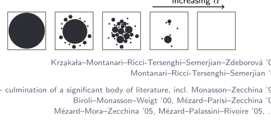
RSB: Condensation (11/22)
In physics picture,
non-concentration
KMRSZ ’07, MRS ’08due to
clustering
followed by
condensation
:
(with k fixed)increasingα
black disk = solution cluster
well-connected clustered condensed UNSAT
αclust αcond αsat
E
Z
¸
(cluster size)
exp
t
ns
u
E
r
number of clusters of that size
s
exp
t
n
Σ
p
s
qu
Ð
maximizer
s
p
α
q
Condensation threshold
: Where
α
cond,
s
Σ
p
s
q
is maximized
with
Σ
p
s
q
0
. After
α
cond, biggest contribution from
exponentially rare clusters.
Solution
: Count clusters rather than solutions.
RSB: Condensation (11/22)
In physics picture,
non-concentration
KMRSZ ’07, MRS ’08due to
clustering
followed by
condensation
:
(with k fixed)increasingα
black disk = solution cluster
well-connected clustered condensed UNSAT
αclust αcond αsat
heuristic implementation of the definition in terms of pure state decomposition (see Eq.4). Generalizing the results of ref. 16, it is possible to show that the two calculations provide identical results. However, the first one is technically simpler and under much better control. As mentioned above we obtain, for allk!4 a value of"d(k) larger than the one quoted in refs. 6 and 11.
Further we determined the distribution of cluster sizeswn, thus
unveiling a third ‘‘condensation’’ phase transition at"c(k)!"d(k) (strict inequality holds fork!4 in SAT andq!4 in coloring, see below). For"!"c(k) the weightswnconcentrate on a logarithmic
scale [namely,"logwnis#(N) with#(N1/2) fluctuations]. Roughly
speaking, the measure is evenly split among an exponential number of clusters.
For " $ "c(k) [and ! "s(k)] the measure is carried by a subexponential number of clusters. More precisely, the ordered sequence {wn} converges to a well known Poisson-Dirichlet process
{w*n}, first recognized in the spin glass context by Ruelle (26). This
is defined byw*n%xn/&xn, wherexn$0 are the points of a Poisson
process with ratex"1"m(")andm(")!(0, 1). This picture is known in spin glass theory as one-step replica symmetry breaking (1RSB) and has been proven in ref. 27 for some special models. The Parisi 1RSB parameterm(") is monotonically decreasing from 1 to 0 when"increases from"c(k) to"s(k) (see Fig. 3).
Remarkably, the condensation phase transition is also linked to an appropriate notion of correlation decay. Ifi(1), . . . ,i(n)![N] are uniformly random variable indices, then, for"!"c(k) and any fixedn:
!
!
'xi!(
"#)xi)1*. . .xi)n**$#)xi)1**. . .#)xi)n**"30 [5]
asN3+. Conversely, the quantity on the left side of Eq.5remains positive for"$"c(k). It is easy to understand that this condition is even weaker than the extremality one (compare Eq.3) in that we probe correlations of finite subsets of the variables. In the next two sections we discuss the calculation of"dand"c.
Dynamic Phase Transition and Gibbs Measure Extremality.A rigorous calculation of"d(k) along any of the two definitions provided above (compare Eqs.3and4) remains an open problem. Each of the two
approaches has, however, an heuristic implementation that we shall now describe. It can be proved that the two calculations yield equal results as further discussed in the last section.
The approach based on the extremality condition in Eq.3relies on an easy-to-state assumption and typically provides a more precise estimate. We begin by observing that, because of the Markov structure of#!, it is sufficient for Eq.3to hold that the same condition is verified by the correlation betweenxiand the set
of variables at distance exactly!fromi, that we shall keep denoting asx!. The idea is then to consider a large yet finite neighborhood ofi. Given!"!!, the factor graph neighborhood of radius!"around
iconverges in distribution to the radius-!"neighborhood of the root in a well defined random tree factor graphT.
For coloring of random regular graphs, the correct limiting tree modelTis coloring on the infinitel-regular tree. For random
k-SAT,Tis defined by the following construction. Start from the root variable node and connect it to l new function nodes (clauses),lbeing a Poisson random variable of meank". Connect each of these function nodes withk"1 new variables and repeat. The resulting tree is infinite with nonvanishing probability if"$ 1/k(k"1). Associate a formula to this graph in the usual way, with each variable occurrence being negated independently with probability 1/2.
The basic assumption within the first approach is that the extremality condition in Eq.3can be checked on the correlation between the root and generation-!variables in the tree model. On the tree,#!is defined to be a translation invariant Gibbs measure (17) associated to the infinite factor graphjT(which provides a specification). The correlation between the root and generation-!
variables can be computed through a recursive procedure (defining a sequence of distributionsP"!, see Eq. 15 below). The recursion can be efficiently implemented numerically yielding the values pre-sented in Table 1 fork(resp. q)%4, 5, 6. For largek(resp. q) one can formally expand the equations onP!and obtain:
"d)k*%2
k
k
#
log k,log logk&'d&O$
log logk
logk
%&
[6]ld)q*%q-logq&log logq&'d&o)1*. [7]
with'd%1 (under a technical assumption of the structure ofP!). The second approach to the determination of"d(k) is based on the ‘‘cavity method’’ (6, 25). It begins by assuming a decomposition in pure states of the form4with two crucial properties: (i) if we denote byWnthe size of thenth cluster (and hencewn%Wn/&Wn),
then the number of clusters of sizeWn%eNsgrows approximately
aseN&(s); (ii) for each single-cluster measure#
n!, a correlation
decay condition of the form3holds.
The approach aims at determining the rate function&(s), com-plexity: the result is expressed in terms of the solution of a distributional fixed point equation. For the sake of simplicity we
jMore precisely#!is obtained as a limit of free boundary measures.
α
d,+α
dα
cα
sFig. 2. Pictorial representation of the different phase transitions in the set of solutions of a rCSP. At"d,,some clusters appear, but for"d,,!"!"dthey comprise
only an exponentially small fraction of solutions. For"d!"!"cthe solutions are split among abouteN&"clusters of sizeeNs". If"c!"!"sthe set of solutions
is dominated by a few large clusters (with strongly fluctuating weights), and above"sthe problem does not admit solutions any more.
Σ(s)
s
αs(k)
αc(k)
m(α)
1
0.5
0
Fig. 3. The Parisi 1RSB parameterm(") as a function of the constraint density
". In theInset, the complexity&(s) as a function of the cluster entropy for"%
"s(k)"0.1 [the slope at&(s)%0 is"m(")]. Both curves have been computed
from the largekexpansion.
10320 " www.pnas.org'cgi'doi'10.1073'pnas.0703685104 Krza¸kałaet al.
heuristic implementation of the definition in terms of pure state decomposition (see Eq.4). Generalizing the results of ref. 16, it is possible to show that the two calculations provide identical results. However, the first one is technically simpler and under much better control. As mentioned above we obtain, for allk!4 a value of"d(k) larger than the one quoted in refs. 6 and 11.
Further we determined the distribution of cluster sizeswn, thus
unveiling a third ‘‘condensation’’ phase transition at"c(k)!"d(k) (strict inequality holds fork!4 in SAT andq!4 in coloring, see below). For"!"c(k) the weightswnconcentrate on a logarithmic
scale [namely,"logwnis#(N) with#(N1/2) fluctuations]. Roughly
speaking, the measure is evenly split among an exponential number of clusters.
For " $ "c(k) [and ! "s(k)] the measure is carried by a subexponential number of clusters. More precisely, the ordered sequence {wn} converges to a well known Poisson-Dirichlet process
{w*n}, first recognized in the spin glass context by Ruelle (26). This
is defined byw*n%xn/&xn, wherexn$0 are the points of a Poisson
process with ratex"1"m(")andm(")!(0, 1). This picture is known in spin glass theory as one-step replica symmetry breaking (1RSB) and has been proven in ref. 27 for some special models. The Parisi 1RSB parameterm(") is monotonically decreasing from 1 to 0 when"increases from"c(k) to"s(k) (see Fig. 3).
Remarkably, the condensation phase transition is also linked to an appropriate notion of correlation decay. Ifi(1), . . . ,i(n)![N] are uniformly random variable indices, then, for"!"c(k) and any fixedn:
!
!
'xi!(
"#)xi)1*. . .xi)n**$#)xi)1**. . .#)xi)n**"30 [5]
asN3+. Conversely, the quantity on the left side of Eq.5remains positive for"$"c(k). It is easy to understand that this condition is even weaker than the extremality one (compare Eq.3) in that we probe correlations of finite subsets of the variables. In the next two sections we discuss the calculation of"dand"c.
Dynamic Phase Transition and Gibbs Measure Extremality.A rigorous calculation of"d(k) along any of the two definitions provided above (compare Eqs.3and4) remains an open problem. Each of the two
approaches has, however, an heuristic implementation that we shall now describe. It can be proved that the two calculations yield equal results as further discussed in the last section.
The approach based on the extremality condition in Eq.3relies on an easy-to-state assumption and typically provides a more precise estimate. We begin by observing that, because of the Markov structure of#!, it is sufficient for Eq.3to hold that the same condition is verified by the correlation betweenxiand the set
of variables at distance exactly!fromi, that we shall keep denoting asx!. The idea is then to consider a large yet finite neighborhood ofi. Given!"!!, the factor graph neighborhood of radius!"around
iconverges in distribution to the radius-!"neighborhood of the root in a well defined random tree factor graphT.
For coloring of random regular graphs, the correct limiting tree modelTis coloring on the infinitel-regular tree. For random
k-SAT,Tis defined by the following construction. Start from the root variable node and connect it to l new function nodes (clauses),lbeing a Poisson random variable of meank". Connect each of these function nodes withk"1 new variables and repeat. The resulting tree is infinite with nonvanishing probability if"$ 1/k(k"1). Associate a formula to this graph in the usual way, with each variable occurrence being negated independently with probability 1/2.
The basic assumption within the first approach is that the extremality condition in Eq.3can be checked on the correlation between the root and generation-!variables in the tree model. On the tree,#!is defined to be a translation invariant Gibbs measure (17) associated to the infinite factor graphjT(which provides a specification). The correlation between the root and generation-!
variables can be computed through a recursive procedure (defining a sequence of distributionsP"!, see Eq. 15 below). The recursion can be efficiently implemented numerically yielding the values pre-sented in Table 1 fork(resp. q)%4, 5, 6. For largek(resp. q) one can formally expand the equations onP!and obtain:
"d)k*%2
k
k
#
log k,log logk&'d&O$
log logk
logk
%&
[6]ld)q*%q-logq&log logq&'d&o)1*. [7]
with'd%1 (under a technical assumption of the structure ofP!). The second approach to the determination of"d(k) is based on the ‘‘cavity method’’ (6, 25). It begins by assuming a decomposition in pure states of the form4with two crucial properties: (i) if we denote byWnthe size of thenth cluster (and hencewn%Wn/&Wn),
then the number of clusters of sizeWn