R E S E A R C H A R T I C L E
Open Access
Bayesian model selection techniques as
decision support for shaping a statistical
analysis plan of a clinical trial: An example from
a vertigo phase III study with longitudinal
count data as primary endpoint
Christine Adrion
*and Ulrich Mansmann
Abstract
Background: A statistical analysis plan (SAP) is a critical link between how a clinical trial is conducted and the clinical study report. To secure objective study results, regulatory bodies expect that the SAP will meet requirements in pre-specifying inferential analyses and other important statistical techniques. To write a good SAP for model-based sensitivity and ancillary analyses involves non-trivial decisions on and justification of many aspects of the chosen setting. In particular, trials with longitudinal count data as primary endpoints pose challenges for model choice and model validation. In the random effects setting, frequentist strategies for model assessment and model diagnosis are complex and not easily implemented and have several limitations. Therefore, it is of interest to explore Bayesian alternatives which provide the needed decision support to finalize a SAP.
Methods: We focus on generalized linear mixed models (GLMMs) for the analysis of longitudinal count data. A series of distributions with over- and under-dispersion is considered. Additionally, the structure of the variance components is modified. We perform a simulation study to investigate the discriminatory power of Bayesian tools for model criticism in different scenarios derived from the model setting. We apply the findings to the data from an open clinical trial on vertigo attacks. These data are seen as pilot data for an ongoing phase III trial. To fit GLMMs we use a novel Bayesian computational approach based on integrated nested Laplace approximations (INLAs). The INLA methodology enables the direct computation of leave-one-out predictive distributions. These distributions are crucial for Bayesian model assessment. We evaluate competing GLMMs for longitudinal count data according to the deviance information criterion (DIC) or probability integral transform (PIT), and by using proper scoring rules (e.g. the logarithmic score).
Results: The instruments under study provide excellent tools for preparing decisions within the SAP in a transparent way when structuring the primary analysis, sensitivity or ancillary analyses, and specific analyses for secondary endpoints. The mean logarithmic score and DIC discriminate well between different model scenarios. It becomes obvious that the naive choice of a conventional random effects Poisson model is often inappropriate for real-life count data. The findings are used to specify an appropriate mixed model employed in the sensitivity analyses of an ongoing phase III trial.
*Correspondence: [email protected]
Institute for Medical Information Sciences, Biometry and Epidemiology (IBE), Ludwig-Maximilians University, Marchioninistr. 15, 81377 Munich, Germany
Conclusions: The proposed Bayesian methods are not only appealing for inference but notably provide a
sophisticated insight into different aspects of model performance, such as forecast verification or calibration checks, and can be applied within the model selection process. The mean of the logarithmic score is a robust tool for model ranking and is not sensitive to sample size. Therefore, these Bayesian model selection techniques offer helpful decision support for shaping sensitivity and ancillary analyses in a statistical analysis plan of a clinical trial with longitudinal count data as the primary endpoint.
Keywords: Statistical analysis plan, Sensitivity analysis, Longitudinal count data, Bayesian generalized linear mixed models, INLA, Predictive performance, Bayesian model evaluation, Informed model choice
Background
A statistical analysis plan (SAP) is a critical link between how a clinical trial is conducted and the clinical study report. To secure objective study results, regulatory bodies expect that the SAP will meet requirements in pre-specifying inferential analyses and other important statis-tical techniques. Writing a good SAP for a model-based sensitivity or ancillary analysis [1,2] involves non-trivial decisions on and justification of many aspects of the cho-sen model setting. In particular, trials with longitudinal count data as primary endpoint pose challenges for model choice and model validation. This paper explores tools for this decision process when sensitivity analyses are per-formed using generalized linear mixed models (GLMMs) for the analysis of longitudinal count data. These tools can be used to build transparent strategies for shaping the final models reported in the SAP.
The documentation of longitudinal profiles for the pri-mary endpoint offers many advantages. They are more informative compared with a single timepoint analysis and give information about the ’speed of efficacy’ [3]. Treat-ment effects evaluated by comparing change over time in quantitative outcome variables between the treatment groups are of great interest [4,5]. The analysis of longitu-dinal profiles offers an effective way to handle composite endpoints like: (1.) the long-term effect of experimental treatment (E) is better than that of standard treatment (S), and (2.) patients under E reach a pre-specified effect faster than those under S.
We are interested in parametric modeling approaches for quantifying absolute effects, adjusting for baseline covariates and handling stratification. There is a rich lit-erature on nonparametric methods for longitudinal data, for example, Brunner et al. [6]. These models do, in general, allow estimation of relative effects. Omaret al. [7] provide an overview of several alternative parametric approaches in trying to deal with individual longitudi-nal profiles: (i) the ’summary statistic method’ [8] using a suitable summary measure (e.g. rates of change, post-treatment mean, last value of the outcome measure, or area under a curve) calculated for each subject, and subse-quently analyzed with rather simple statistical techniques; (ii) repeated measures analysis of variance; (iii) marginal
models based on generalized estimating equations (GEE) [9]; (iv) mixed effects modeling approach involving fixed and random effects components [10,11].
Mixed effects (or random effects) models allow us to investigate the profile of individual patients, estimate patient effects and describe the heterogeneity of treatment effects over individual patients. They account for differ-ent sources of variation (patidiffer-ent effects, cdiffer-enter effects, measurement errors) and provide direct estimates of the variance components which might be of interest in their own right. Furthermore, they allow us to address various covariance structures and are useful for accommodating overdispersion often observed among count response data [10-12].
The EMA Guideline on Missing Data in Confirma-tory Clinical Trials from 2010 [13] explicitly considers random effects approaches (i.e. generalized linear mixed effects models (GLMMs) in the case of a non-Gaussian response) as an approach to handling trials with a series of primary endpoints measured repeatedly over time. Mixed models are also helpful for handling missing values. They are applicable under missing completely at ran-dom (MCAR) as well as missing at ranran-dom (MAR) [14], while simple repeated univariate analyses for each time point using test procedures such as thet-test, ANOVA, or the Wilcoxon rank sum test rely on the more restrictive assumption of MCAR. Also, for non-ignorable missing data mechanisms, newer model-based strategies for lon-gitudinal analyses are increasingly available and offer the opportunity to account for dropout patterns (e.g. pat-tern mixture models [15]). To be fully compatible with the intention-to-treat (ITT) principle, one has to explic-itly consider incomplete individual profiles to correctly incorporate the information available for all randomized patients.
specifying a GLMM for the analysis. Consideration should mainly be given to the following issues:
(i) Distributional assumptions: Poisson, negative binomial, or more sophisticated extensions, e.g., accounting for zero-inflation.
(ii) Transformation of outcome variable: e.g.
log-transformation for skewed continuous positive variables [18], or variance-stabilizing transformations (e.g. inverse hyperbolic sine-transformation for non-negative count variables). An FDA guideline [19] postulates that a rationale for the choice of data transformation along with the interpretation of the estimates of treatment effects based on the transformed scale should be provided. In some situations, transformation of endpoint data is
indicated and preferred to untransformed analyses on the original scale. However, careful consideration should be given to using a transformation which should be pre-specified at the protocol design stage. (iii) Variance-covariance structure: specifying whether
random effects (e.g. patient-specific intercept, patient-specific slopes) are appropriate; specification of the within-error structure. Altogether, random effects selection can be challenging, particularly when the outcome distribution is not normal (see [20-22] for more details).
(iv) Methods for handling dropouts: e.g. dealing with informative drop-outs, applying an analysis in which the last observation is carried forward, accounting for non-ignorable missing data mechanisms
(pattern-mixture models). This approach must be fully compatible with the intention-to-treat principle. (v) Use of covariate- or baseline-adjusted analyses,
handling multi-center data: specifying the mean structure by identifying the fixed effects terms.
The last issue is proposed by Pococket al.[23] for avoid-ing misuse and data-driven selection of covariates within the clinical trial setting. The typical strategy for settling this complex issue is to decide on a simple model on which the primary analysis is based and to use sensitivity anal-yses to assess the robustness of the derived result under realistic model deviations.
In this paper, we propose using pilot or pre-study data to make aninformed choiceabout the sensitivity analysis stated in the SAP. Pilot or pre-study (commonly called a “feasibility” or “vanguard” study) data come from a trial in an earlier phase, from a registry, or from a proof-of-concept study. For phase III trials, data from phase II trials generally exist [24]. In this respect we could also use data from the comparable treatment arms of related studies. Using these data helps to shape and justify in advance the modeling strategy for analyzing the main
trial data, and to check the validity and the appropri-ateness of several model assumptions. It is imperative to minimize misspecification of the assumed GLMM, and this analysis enables the trial statistician to define a broad and robust setting for the final choice of the model.
Having determined the main focus of this paper, we need to motivate our choice ofBayesiantools for achiev-ing our goal. Within the GLMM framework, analytical methods for model assessment and goodness-of-fit cri-teria are not straightforward, andfrequentistapproaches remain limited. The inclusion of random effects makes theoretical derivations rather complex, imposing com-putational challenges. Some proposed model evaluation procedures focus on checking the deterministic compo-nents (i.e. mean and variance-covariance structure) of a GLMM based on the cumulative sums of residuals, or assess the overall adequacy by means of a goodness-of-fit statistic which can be used in a manner similar to the well-known R2 criterion [25,26]. Furthermore, for small sample sizes, likelihood-based inference via penal-ized quasi-likelihood in the case of a longitudinal discrete outcome can be unreliable with variance components being difficult to estimate. In contrast, many easy-to-implement tools are available within theBayesian frame-work. We will briefly review Bayesian tools developed recently and demonstrate their usefulness: For assess-ing goodness-of-fit and performassess-ing model validation, we apply the probability integral transform (PIT) [27-29] as a graphical posterior model check. We implement formal statistical criteria such as the deviance information cri-terion (DIC) [30], conditional predictive ordinate (CPO) [31,32], or proper scoring rules [28,29,33-36] to compare the forecasting capability of different competing GLMMs. A further objective is exploring the behavior of these dif-ferent Bayesian methods for model validation concerning the coherence of their preference for a certain candidate model.
Supplementary Material of this paper [see Additional files 1 and 2].
For data analysis, inla-program [38] based on the open-source software R version 2.12.1 [39] was used to demonstrate the applicability of the Bayesian toolbox.
Methods
Bayesian generalized linear mixed models for longitudinal count data
In the following, regression approaches to modeling dis-crete count outcomes are briefly outlined. In the clinical trial setting, we assume that each patienti,i = 1,. . .,N, is randomized to a new drug (xi= 1) or a standard
treat-ment (xi = 0). The observationsyij for each patient are
counts measured in the course of time during each study visit,j=1,. . .,ni(presuming an imbalanced design), with
timetij∈Randti1=0. The linear predictor is defined as ηij=(β0+b0i)+(β1+b1i)tij+β2xi+β3xitij, (1)
with β=(β0,β1,β2,β3)T being the population-level parameter vector (fixed effects), b0i denoting
patient-specific random intercepts and b1i subject-by-visit
ran-dom slopes. The fixed effects (in a frequentist framework) account for group-specific effects (e.g. treatment group or time), serving at the same time as parameters of interest in a clinical trial. We want to relate the count response to explanatory variables such as time and treat-ment. In the most general case, a standard assumption for a GLMM with both random intercept and slope is that bi = (b0i,b1i)Tfollows a bivariate normal
distribu-tion with mean zero and an unknown precision matrix
Q=Q(φ)depending on parametersφ, i.e.
bi|Q∼iidN2(0,Q−1).
The variance covariance matrixQ−1for variance com-ponentsφis parameterized in terms of precisions and a correlation parameter. That is,
Q−1=
1/τb0i ρ/
√τ
b0iτb1i ρ/√τb0iτb1i 1/τb1i
,
whereτ.refers to the marginal precision of random effects b.i. Therefore, it is necessary to allow for the correlation
ρbetween random intercepts and slopes. In GLMMs for-mulated within a Bayesian framework, a non-Gaussian hyperprior distribution must be assigned to the precision matrixQ(φ), whereτ.andρrepresent the hyperparame-ters. As proposed by Fonget al.[40] and Wakefield [41], we assume
Q∼Wishart2(r,R−1).
The prior parameters of the Wishart prior are
(r,R11,R22,R12), wherer > 1 (to obtain a proper prior)
in the case of two dependent random effects.R12 is ele-ment (1, 2) of the inverse of R and R12 = R21 be-cause of symmetry. Integration overQgives a marginal t2(0, [(r−1)]−1R,r−1)-distribution ofbi = (b0i,b1i)T,
witht2denoting the Student’stdistribution with 2 degrees of freedom.
Poisson GLMM
Poisson loglinear regression is a common choice for mod-eling count response data. The probability function can be expressed as
Prμ(y)=exp(−μ)μy/y!
fory= 0, 1, 2,. . .andμ >0. For longitudinal count data withi = 1,. . .,N subjects andj = 1,. . .,ni
measure-ments per subject, the observed countsyijare
condition-ally independent Poisson variablesYij∼Poi(μij), with the
conditional mean ofYij related to the linear predictor by
a logarithmic link function. Letμij= E(Yij|β,bi). Hence,
the resulting predictor in a standard Poisson GLMM for predicting the mean rate is
log(μi)=ηi=Xiβ+Zibi,
whereXiis anni×pmatrix andZiis anni×qmatrix,
withβap×1 vector of population-level parameters (fixed effects) and bi a q × 1 vector of zero-mean normally
distributed random effects. In the longitudinal setting described in equation (1),p= 4,q = 2 andZi = (1,ti).
The primary Poisson assumption is equidispersion, i.e. the equality of the mean and the variance functions. However, this is often inconsistent with empirical evidence. In real-ity, the value of the variance often exceeds that of the mean
μij, resulting in overdispersion. Thus, although they are
widely used to model count data, Poisson GLMMs may not well be suited to types of count outcomes from specific applications.
Negative binomial GLMM
A conventional modeling approach for overdispersed count data where the variance exceeds the mean (i.e. a given rate μij) is the negative binomial (NB) loglinear
regression. In the classical univariate setting (dropping the subscripti), the NB density can be written as
Prk,p(y)= (
y+k)
(k) (y+1)p
k(1−p)y,
parameter. For negative binomial data, the corresponding mean and variance are then given by
μ= k(1−p)
p and σ
2=μ+μ2/k= k(1−p) p2 ,
withp=k/(k+μ)=μ/σ2, k=μ2/(σ2−μ).
Overdispersion in the negative binomial model can be interpreted by unobserved heterogeneity among the observations y. If this phenomenon is not taken into account in the modeling process, it can lead to underes-timated variance which then leads to incorrect posterior inference. It must be kept in mind that in the NB regres-sion, the dispersion parameter takes observation-specific values. In the limitk → ∞, holdingμfixed, the variance approaches the mean and therefore the negative bino-mial NB(k,p)converges to Poi(μ)(withμ = k1−pp) in a distributional manner.
Zero-inflated GLMM
In many biometrical and epidemiological applications, the count data encountered often contain a high propor-tion of extra zeros relative to the Poisson distribupropor-tion, which is routinely applied for these situations. Therefore, a major source of overdispersion in these situations is a preponderance of zero counts.Zero-inflatedcount mod-els provide a parsimonious yet powerful way to model this type of situation. Such models assume that the data originate from a mixture of two separate processes: one generates only zeros, and the other is either a Poisson or a negative binomial data-generating process. The result of a Bernoulli trial is used to determine which of the two processes generates an observation.
Hence, as regards zero-inflated estimation method in general, two regression equations are created: one predict-ing whether the count occurs (“always zero group”) and a second predicting differences in the occurrence of the count (“not always zero group”). While these differences are not modeled with standard Poisson or negative bino-mial regression, zero-inflated models first account for the excessive zeros by predicting group membership – i.e. an unobserved latent dichotomous outcome – based on the constellation of covariates included in the model and then predicting frequency of counts for only those in the “not always zero group”. The zero-inflated version of a distri-bution Dof a random variable Y ∼ ZID(π0,θ), where ZID denotes a zero-inflated distribution, has a probability function of the form
fZID(y)=π0I[y=0]+(1−π0)fD(y;θ),
wherefD(y|θ)is the probability function of distributionD
with parameters θ. Hence,fZID(y) exhibits an additional, zero-inflation hyperparameter π0 for the proportion of
additional zeros. From the equation above, the probabil-ity of zero is equal toπ0+(1−π0)fD(y=0|θ), while the
probability ofy>0 is given by(1−π0)fD(y|θ).
Two popular models that account for data with excess zeros are the inflated Poisson (ZIP) and the zero-inflated negative binomial (ZINB). The ZIP distribution introduced by Lambert [42] is the simplest ZID.
In the longitudinal setting, the full ZIP mixed effects model has the following representation:
Yij∼ZIP(π0ij,μij) and
Yij∼
0, with probabilityπ0,ij
Poi(μij), with probability(1−π0,ij).
A ZIP model will reflect the data accurately when overdispersion is caused by an excess of zeros. In gen-eral, a ZIP mixed effects model can be used when one is not certain about the nature of the source of zeros, and observations are overdispersed and simultaneously corre-lated because of the sampling design or the data collection procedure. By contrast, if overdispersion is attributed to factors beyond the inflation of zeros, a ZINB model is more appropriate [43]. Furthermore, the rate of zero-inflation may change over time. This problem goes beyond the scope of this paper, and we focus on ZIP GLMMs as an alternative to the Poisson GLMM generally used for ana-lyzing longitudinal counts. More details concerning these issues can be found in Hilbe [44] or Lambert [42].
Again, a Bayesian approach provides an easy way to deal with zero-inflated hierarchical count data by incorporat-ing a prior forπ0(generally beta prior or a uniform prior when no information is available). For longitudinal data with repeated observations, the correlation structure may be taken into account by introducing random effects in the proposed zero-inflated model. More details can be found in Dagne [45] or Ghoshet al.[46].
NMM with variance-stabilizing transformation
It is not uncommon for a regression model to be inap-propriate for a given response variable but reasonable for some transformation provided that it is methodolog-ically justified. For a longitudinal count outcome, this means that anormalmixed effects model (NMM) should be considered as an alternative modeling strategy, with an assumption of Gaussian errors on the transformed scale: an inverse hyperbolic sine-transformation [47] of the responseyvia
arcsinh(y)=log(y+
y2+1)
the Appendix A1. This approach is motivated by analyz-ing the data with a robust and well-understood algorithm as regards parameter estimation. Particularly in a fre-quentist framework, likelihood-based inference is far less straightforward for GLMMs than it is for NMMs. Analyt-ical intractability is the reason why a variety of numerAnalyt-ical integration techniques for maximizing the likelihood have been developed (e.g. Gauss quadrature or penalized quasi-likelihood). In a Bayesian framework, computation is a major issue for complex hierarchical GLMMs since the usual implementation based on the Markov chain Monte Carlo (MCMC) method tends to exhibit poor perfor-mance, lack of convergence or slow mixing properties when applied for such models. As regards computational cost, NMMs clearly outperform mixed models for non-Gaussian response.
Bayesian inference using the INLA approach
For Bayesian GLMMs, an analytical computation of the posterior marginals of the unknown fixed parameters and hyperparameters is not possible: The posterior marginals are not available in closed form because of the non-Gaussian outcome. Hence, the standard approach used to obtain posterior estimates are MCMC methods [48-50]. However, within the MCMC framework several problems in terms of both convergence and computational time occur in practical applications. Recently, Rue et al. [37] proposed an approximate alternative for parameter esti-mation in a subclass of Bayesian hierarchical models, the so-calledlatent Gaussian models. These are models with a structured additive predictor
ηi=α+ nf
l=1
f(l)(uli)+ nβ
g=1
βgxgi+i, (2)
wheref(l)(·)represents an unknown function of continu-ous covariatesu, comprising for example nonlinear effects of covariates, time trends, spatial dependencies, or inde-pendent identically distributed individual-level parame-ters (random effects). Theβg’s denote the linear effect of
some covariates x, and the i’s are unstructured terms.
Gaussian priors are assigned toα,f(l)(·),βgand, whereas
the priors for the hyperparameters φ do not have to be Gaussian. Random effects are introduced by defining f(ui)=fiand letting{fi}be independent, have zero mean
and be Gaussian distributed. INLA is a new computa-tional approach to statistical inference for latent Gaussian Markov random field (GMRF) models that can bypass MCMC. Known problems with MCMC no longer apply using INLA as no Monte Carlo inference is involved. The theoretical background and computational issues are described in detail in Rueet al.[37,51]. In short, a latent GMRF model, which underlies INLA, is a hierarchical model which can be characterized through three stages. In
the first stage, the distributional assumption is formulated for the observablesyi, usually assumed to be conditionally
independent given some latent parameters and, possibly, some additional hyperparameters. In the second stage, an a priori model for the unknown parameters is assigned and the corresponding GMRF is specified. The third and last stage of the model consists of determining the prior distributions for the hyperparameters. With this method, a recipe for fast Bayesian inference using accurate, deter-ministic approximations to the marginal posterior den-sity for the hyperparameters and the marginal posterior densities for the latent variables is provided in a fully automated way. The INLA computational approach com-bines Laplace approximations and numerical integration in a very efficient manner. Three types of approximation are available: Gaussian, full Laplace, or simplified Laplace approximation. Each of these approaches has different features varying in accuracy and computational cost. In this article, we used the full Laplace approximation for the numerically inaccessible integrals of the posterior marginal density as this approximation is supposed to be the most accurate [37,52].
Using the INLA approach it is also possible to challenge the model itself. For example, a set of competing GLMMs can be assessed through cross-validation in a reason-able time without reanalyzing the model after omission of observation yij. Hence, within the INLA framework,
GLMMs can be fitted at low computational cost, giving access to various predictive measures for model compar-ison. Additionally, this approach facilitates the validation of distributional assumptions concerning the model being studied.
Details on how to use the open-source softwareinla
can be found in the manual offered by Martino and Rue [38] or [53], and on the website www.r-inla.org. The inla-program, written in C and bundled within an R-interface [39] called R-INLA, can be down-loaded from the webpage for Windows, MAC and Linux, or simply by typing the following command line within R source("http://www.math.ntnu.no/
inla/givemeINLA.R"). Accordingly, R-INLA
per-mits model specification and post-processing of results directly inR. All analyses in this paper were run using the
R-INLApackage built in October 2011.
Methods for model assessment and comparison
data and to firmly establish the model’s credibility (model assessment). For example, we can check whether a spe-cific random effect at a certain grouping level is war-ranted or whether it can be eliminated. To identify model deficiencies and facilitate model comparison and model selection, several Bayesian tools recently proposed by var-ious authors are available. These tools can be applied to addressing the issue of predictive performance of a model, or to identify model deficiencies and to detect possible outliers or surprising observationsyijthat do not fit the
given model and may require further attention. Addi-tionally, methods for model comparison should provide information about which model performs best.
Deviance information criterion (DIC)
Appropriate statistical selection of the best model from a collection of hierarchical GLMMs is problematic mainly because of ambiguity in the “size” of such models arising from the shrinking of their random effects towards a com-mon value. To address this problem, Spiegelhalteret al. [30] suggest DIC as a generalization of the Akaike infor-mation criterion (AIC) which can be used as a Bayesian approach for model comparison and to assess the ade-quacy of hierarchical models. DIC compares the global performance and predictive accuracy of different alterna-tive models accounting for model complexity. Like AIC, the basic idea of DIC is a trade-off between model fit and model complexity. Models with more parameters tend to fit the data better than models with less parameters. How-ever, a larger set of parameters makes the model more complex with the danger of overfitting. Hence, model selection should account for both goodness-of-fit and complexity of the model. The smaller the DIC the bet-ter the trade-off between model fit and complexity. The model with the smallest DIC is considered to be the model that would best predict a replicate data set of the same structure as that currently observed. DIC is based on the posterior distribution of theBayesian deviancestatistic,
D(θ)= −2 logf(y|θ)+2 logh(y), (3)
where f(y|θ) is the likelihood function for the observed data vector ygiven the parameter vector θ, andh(y) is some standardizing function of the data (thus not hav-ing an impact on model selection). In this approach, the fit of a model is summarized by the posterior expectation of the devianceD¯ = Eθ|y[D], while the complexity of a
model is captured by the effective number of free param-eterspD, which is typically less than the total number of
parameters. For non-hierarchical models, pD should be
approximately the true number of parameters.pDcan be
thought of as the“posteriori mean of the deviance”minus the“deviance evaluated at the posterior means”
pD=Eθ|y[D]−D(Eθ|y[θ])=D(θ)−D(θ)¯ .
DIC is then defined as
DIC=2D¯ −D(θ)¯ =D(θ)¯ +2pD
= ¯D+pD, (4)
DIC is scale-free. Because of the standardizing func-tion h(y) in (3), DIC values have no intrinsic meaning, and only differences in DIC across candidate models are meaningful. The question of what constitutes a notewor-thy difference in DIC between two candidate models has not yet received a satisfactory answer. Differences of 3 to 5 are normally being thought of as the smallest that are still noteworthy [49,50].
Spiegelhalteret al.[30] and Plummer [54] discuss some limitations of DIC: Although widely used, DIC lacks a clear theoretical foundation. It can be shown that DIC is an approximation of a penalized loss function based on the deviance, with a penalty from a cross-validation argument. However, this approximation is valid only when the effective number of parameters in the model is much smaller than the number of independent observations. The ratiopd/nmay be used as an indicator of the validity
of DIC. In disease mapping or random effects models for longitudinal data this assumption often does not hold and therefore DIC under-penalizes more complex models.
Computational details DIC is simple to calculate using MCMC simulation and is routinely implemented in Win-BUGS [55-58]. With the INLA approach, both compo-nents of DIC, pD and D, can be computed by setting¯
the option dic = TRUE in the control.compute
statement within theinla(.)-call. For further details see [37].
Conditional predictive ordinate (CPO)
As a device for detecting possible outliers or surpris-ing observationsyijwithin a posited model and therefore
checking the model fit, theconditional predictive ordinate (CPO) for each observation can be computed [59]. To be more precise, this predictive quantity given by
CPOij=π(yij|y−ij) (5)
constitutes the position of the observed value yij within
the leave-one-out cross-validatory posterior predictive distribution evaluated at the observed valueyij. A small
value ofCPOijindicates an observationyijthat is unlikely
under the model fit without the observation in question, i.e. ’surprising’ in the light of the prior knowledge and the other observations [60]. Accordingly, this observation is not expected under the cross-validation posterior predic-tive distribution of the current model. CPO measure is discussed among others by Gelfandet al.[32], Congdon [61] and Gilkset al.[48]. Since for discrete dataCPOijcan
future wheny−ijis already observed, it can be interpreted easily.
Computational details Examination of model
perfor-mance at the level of the individual observation can pro-vide added insight into discovering the reasons for poor global performance. For each observationyijof the model,
we use the value of the cross-validation predictive density at the observed data points as a local discrepancy mea-sure. A plot forCPOijversusijcan be used informally as
a diagnostic tool to reveal surprising observations. With MCMC sampling, calculating the CPO predictive quan-tity requires refitting the model by single case omission. Withinla, CPO can be returned for each observation at low computational cost without rerunning the analysis by using the optioncpo = TRUE. However, in practice, the assumptions behind the numerical computation might fail for some observations. For these points, the CPO values have to be re-computed manually. That is,yijis removed
from the model and simply refitted only computing the posterior marginals for the linear predictor for this obser-vation. (As the results from fitting the whole model can be used to improve e.g. initial values, this process allows a more efficient implementation). For further reading refer to [51].
Proper scoring rules as a toolbox for the assessment of prognostic performance
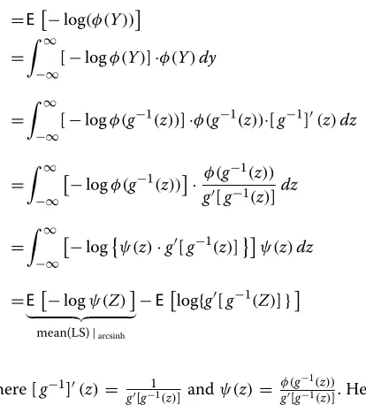
Besides model choice criteria such as DIC, CPO or graph-ical techniques, the comparison and ranking of differ-ent competing models can be based on proper scoring ruleswhich were proposed by Gneiting and Raftery [33] for assessing the quality of probabilistic forecasts (see [34-36,62] for more details). Scoring rules provide a suit-able summary measure for the evaluation of probabilistic forecasts, by assigning a numerical score based on the posterior predictive distribution P and on the event y that materializes. We take scoring rules to be negatively oriented penalties that a forecaster wishes to minimize: Specifically, if the forecaster quotes the predictive dis-tribution P and yis the observed value, the penalty is s(P,y). We writes(P,Q)for the expected value ofs(P,Y), when Y ∼ Q. Models with smaller score values should be preferred to models with larger values. Additionally, propriety is an essential property of a scoring rule that encourages honest and coherent predictions. Gneiting and Raftery [33] contend that the goal of probabilistic forecasting is to maximize the sharpness of the predictive distributions subject to calibration.Calibrationrefers to the statistical consistency between the probabilistic fore-casts and the observations y, and is a joint property of the predictive distributions and the actual observationy. Sharpnessrefers to the concentration of the predictive dis-tribution, and is a property of the forecast only [28,29,63].
Hence, in the context of model comparison, scoring rules provide a diagnostic approach to assessing the predictive performance of a model.
The most prominent example of strictly proper scoring rules is thelogarithmic score[64] which is defined as
LSij= −log(πyij), (6)
where πyij =Pr(Yij = yij|y−ij) indicates the
cross-validated leave-one-out predictive probability mass at the observed value yij, i=1,. . .,N, j=1,. . .,ni. The
sub-script −ij in y−ij denotes that for patient i observation j is removed. Concerning logarithmic score values, the following relationship holds:
LSij= −log(CPOij).
Gneiting and Raftery [33] proposed ranking compet-ing forecast procedures (i.e. competcompet-ing models) on the basis of their mean scores, e.g.LS=(Ni=1ni)−1
i,jLSij,
and not by graphical methods such as boxplots. The difference in the mean scores can be considered since only the mean scores are still proper. Therefore, we want to compare the mean scores of two rival models by using a formal significance test to assess if score differ-ences are statistically significant on a certain level. The paired Monte Carlo permutation test [65,66] based on the observation-level scores provides a convenient approach, as unlike the paired t-test it does not require distribu-tional assumptions (e.g. normality of individual scores) or trust in asymptotic behavior. Permutation tests compare the observed score values, suitably summarized in a test statistic, with randomly permutated score values, which can be viewed as samples under the null hypothesisH0of no difference.
Computational details To calculate the scores in the
MCMC setting, a leave-one-out cross-validation ap-proach using the posterior predictive distribution is the gold standard, obtained by reanalyzing the data with-out a suspect statistical unit. However, full and exact cross-validation is extremely time-consuming in practice and often generally infeasible within an MCMC analysis. Marshall and Spiegelhalter [67] proposed the “full-data mixed approach” (ghost sampling) generating full ’ghost’ sets of random effects for each unit without repeatedly fit-ting the model with one particular observation removed (for more details also compare [68] or [69]).
optioncpo = TRUEin thecontrol.compute state-ment within theinla(.)-call [37,38,51].
Probability integral transform (PIT)
Unusually small values of CPO indicate surprising obser-vations. However, what is meant by ’small’ has to be calibrated to the level of the Gaussian field in order to compare CPO values. One possible calibration procedure is to compute the probability integral transform (PIT) proposed by Dawid [27]. In the univariate case, PIT is a tool for assessing calibration and therefore evaluates the adequacy of a single model.
The PIT value for each single observation is defined as
PITij=Pr(ynewij ≤yij|y−ij), (7)
withy−ijbeing the observation vector with theijth com-ponent omitted, and is simply the value that the pre-dictive cumulative distribution function (CDF) attains at the observation yij. This procedure is performed in
cross-validation mode meaning that in each step of the validation process the ensuing leave-one-out posterior predictive distribution is calculated.
Unusually large or small values of PITij indicate
pos-sible outliers or surprising observations not supported by the model under consideration. If the observation is drawn from the predictive distribution, which is an ideal and desirable situation, and the predictive distribution is continuous, the PIT has a uniform distribution on the unit interval [ 0, 1]. To evaluate whether a data vectory seems to come from a specific distribution, i.e. to check calibration empirically, a histogram of all PIT values can be plotted and checked for uniformity [28,29,33]. A his-togram of the PITs far from the uniform might indicate a questionable model and hint at reasons for forecast fail-ures and model deficiencies. U-shaped histograms indi-cate under-dispersed predictive distributions, inverse-U shaped histograms point at over-dispersion, and skewed histograms occur when central tendencies are biased. In the case of count data, the predictive distribution is discrete resulting in PIT values no longer being uni-form under the null hypothesis of an ideal forecast. To overcome this problem, several authors suggest a “non-randomized” version of PIT values (see [28] for more tech-nical details). Hence, anadjustedPIT can be used instead, defined as
PITij=Pr(ynewij <yij|y−ij)+0.5·Pr(y
new
ij =yij|y−ij), (8)
These adjusted PIT values can be interpreted in exactly the same way as in applications with continuous outcome data. However, when using PIT as a diagnostic tool it has to be considered that PIT does not take into account the sharpness of the density forecast, as opposed to proper scoring rules providing a combined assessment of both calibration and sharpness simultaneously.
Computational details In the MCMC setting,
nonran-domized PIT values for count outcomes are cumbersome and rather time consuming because of the leave-one out cross-validation approach. To reduce the computational burden, the INLA approach can be applied to compute PITij,i=1,. . .,N,j=1,. . .,ni.
Motivating example: vertigo phase III dose-finding study (BEMED trial)
Study synopsis The BEMED trial (Medical treatment
of Meni`ere’s disease with Betahistine; EudraCT No.: 2005-000752-32; BMBF177zfyGT; Trial Registration: Cur-rent Controlled Trials ISRCTN44359668) is an ongo-ing investigator-initiated, multi-center, national, random-ized, double-blind, placebo-controlled, clinical trial with a parallel group design. This dose-finding phase III trial recruiting patients from several dizziness units through-out Germany comprises three arms: therapy with high dose betahistine-dihydrochloride (3 × 48 mg per day) vs. a low dose (2× 24 mg per day) vs. placebo. Total treatment time will be nine months with a three month follow-up. The objective of this study is to evaluate the effects of betahistine in high-dosage vs. low-dosage vs. placebo on the occurrence of vertigo attacks. The study was approved by the local ethics committee and is per-formed in accordance with the International Conference on Harmonization Guidelines for Good Clinical Prac-tice, as well as with the Declaration of Helsinki. Written informed consent was obtained from patients who met the study inclusion criteria.
Design aspects and statistical analyses A sample size of n = 138 patients in total (46 in each group) to be ana-lyzed was considered necessary. The total treatment time will be nine months with a three month follow-up. The primary efficacy outcome is the number of vertigo attacks in the three treatment arms during the last three months of the 9 month treatment period. The primary efficacy analysis is nonparametric and will be performed accord-ing to the ITT principle. The closed testaccord-ing procedure is used to avoid adjusting the significance level. Sensitivity analyses will be performed using a longitudinal approach to quantify patient profiles and the ’speed of efficacy’, i.e., how quickly reduction in attack frequency is achieved in the three treatment groups. For the prospectively speci-fied SAP, it has to be decided which candidate set of mixed effects models proposed at the beginning of the Methods Section seems appropriate for analyzing the counts.
Informed model choice The decision on the models for
population, comparable intervention, and same definition of primary outcome (frequency of vertigo attacks).
Results
Application to clinical trial data
Vertigo pre-study: data and modeling details
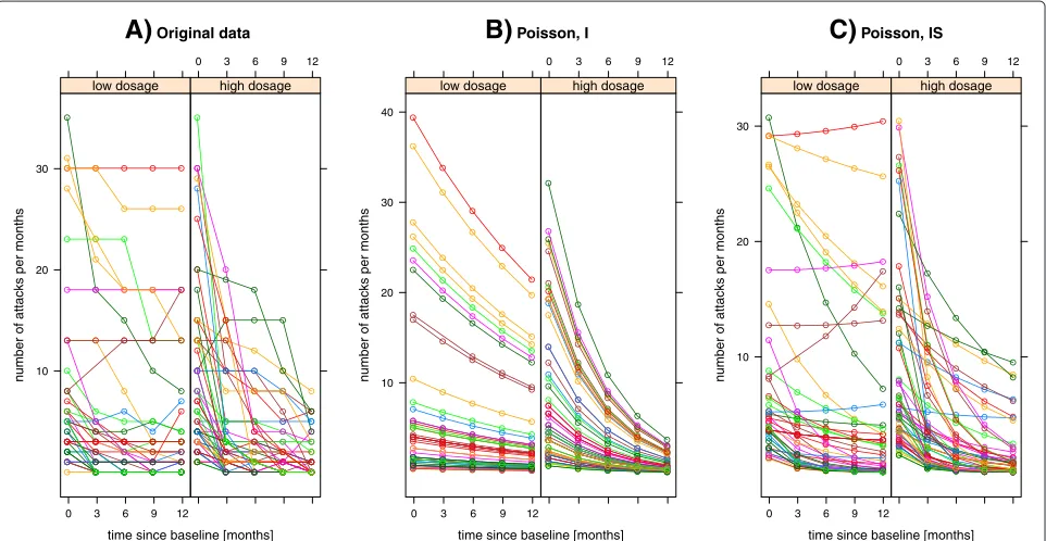
To demonstrate the applicability of the Bayesian tool-box within the GLMM framework, we used real life longitudinal count data from an open, non-masked, exploratorytrial conducted by the dizziness unit, Depart-ment of Neurology, University Hospital Munich, Germany [70]. 112 patients between the ages of 18 and 80 years with Meni`ere’s disease received either a low dosage of betahistine-dihydrochloride, i.e. 16 or 24 mg tid, or a higher dosage of 48 mg tid for at least 12 months. 50 patients were in the low dosage group (coded as zero) and 62 in the high dosage group (coded as one). Both treatment groups did not differ with respect to patient characteristics at baseline measurement (ti1 ≡ t1 = 0, for alli = 1,. . ., 112). In particular, there was no signif-icant difference in the number of attacks at baseline (see [70] for more details). The full dosage was given from the beginning of the treatment. Since the major aim of the treatment of Meni`ere’s disease is reducing the attack frequency, the efficacy outcome variable was the number of vertigo attacks per month during a 3-month period, i.e. during a period of 3 months preceding treatment and then every 3 months for up to 12 months. Follow-up examination every 3 months showed that the mean num-ber of attacks per month decreased in both groups over time, and was significantly lower in the high-dosage than in the low dosage group; the longer the treatment, the greater the difference between the two treatment groups. Longitudinal data are displayed in Figure 1. Moderate ver-tical differences between the individual profiles could be identified.
We consider a count outcome variable, yij, which in
our example represents the number of vertigo attacks per months for the ith patient measured at timetij ≡ tj =
0, 3, 6, 9, 12, for j = 1, 2, 3, 4, 5. To account for between-patient variability we introduced between-patient-level random intercepts as well as patient-specific slopes, and then fitted main effects and interaction models:
ηij=(β0+b0i)+β1timej+β2dosagei·timej model (I) ηij=(β0+b0i)+(β1+b1i)timej+β2dosagei·timej model (IS)
The main effect for a treatment group, defined by
dosagei, was left out of the systematic part since treat-ment effect was expected to happen slowly with time and not in a way that a strong effect is established after a short time and stays stable for the duration of the longitudinal observation.
We considered flexible models allowing for overdisper-sion and zero-inflation, respectively. Hence, both for mod-els of type (I) and (IS), we investigated four different types of GLMM by changing the distributional assumption:
a) Poisson model foryij∼Poi(μij). Poisson GLMM
was used as the “reference model” as this
distributional assumption is often the default choice. b) Zero-inflated Poisson (ZIP) model, which will
explain the mean attack frequency and the
zero-inflation probability (i.e. assuming an excess of zero observations).
c) Negative Binomial (NB) model, as a robust alternative to accommodate substantial extra variation or overdispersion.
d) Normal mixed effects model (NMM), for
arcsinh-transformed outcome “attack frequency” as an alternative modeling strategy to accomplish stabilization of variance.
All models included patient-specific random intercepts b0i|σb−2 ∼iid N(0,σb2), while the need for
patient-specific slopes associated withtimewas investigated for all candidate models. Therefore, for the latter type of GLMM, correlated patient-specific intercepts and slopes being zero mean bivariate normal were assumed, i.e.
(b0i,b1i)T|Q ∼iid N2(0,Q−1). For models of type (I), a
Gamma prior was assigned to the precisionσb−2. Accord-ing to Fonget al.[40], for models of type (IS) we assumed
Qto follow a Wishart2(r,R−1)-distribution withQ = I2. In general, independent zero-mean Gaussian priors with fixed small precisions were assigned to each component of the population-level parameter vectorβ. As the accu-racy of the simplified Laplace approximation is often not sufficient for the computation of predictive measures [52], the full Laplace approximation was chosen in the follow-ing application, in combination with the so-called GRID integration strategy for numerically exploring the approx-imative posterior marginal densities (for more details concerning this issue see [37]).
Vertigo pre-study: analysis results
In Table 1 INLA summaries for the vector of population-level parameters (fixed effects) are described. Addition-ally, 95% credible intervals are reported. These 95% equal-tail intervals correspond to the 2.5% and 97.5% per-centiles of the corresponding posterior distribution and enable assessment of whether, e.g., time profiles of the pri-mary efficacy outcome variable differ in both treatment groups (dosage∗time). We conclude that posterior esti-mates for models of type (I) and of type (IS), respectively, agree between differing distributional assumptions.
A)
Original datatime since baseline [months]
n
u
mber of attacks per months
10 20 30
0 3 6 9 12
low dosage
0 3 6 9 12
high dosage
B)
Poisson, Itime since baseline [months]
n
u
mber of attacks per months
10 20 30 40
0 3 6 9 12
low dosage
0 3 6 9 12
high dosage
C)
Poisson, IStime since baseline [months]
n
u
mber of attacks per months 10
20 30
0 3 6 9 12
low dosage
0 3 6 9 12
high dosage
Figure 1Trajectory plots for vertigo data.Effect of betahistine-dihydrochloride on the frequency of attacks of vertigo in a total of 112 Meni`ere’s disease patients; 2 treatment groups: “low-dosage” (50 patients) vs. “high-dosage” (62 patients).A)individual trajectories for vertigo data.B)andC) display the conditional posterior mean trajectories of the number of attacks depending upon fixed and random effects after fitting a Poisson GLMM (I: model with random intercepts. IS: model with random intercepts and slopes). The same color is used to indicate observations and model-based estimates for the same patient.
time, interaction for treatment group and time, and ran-dom effects are visualized by means of trajectory plots, assuming a Poisson (IS) GLMM. Furthermore, Figure 2 illustrates the approximated posterior marginals for the most important fixed effects by comparing INLA results with those obtained using the MCMC approach (see Appendix A3).
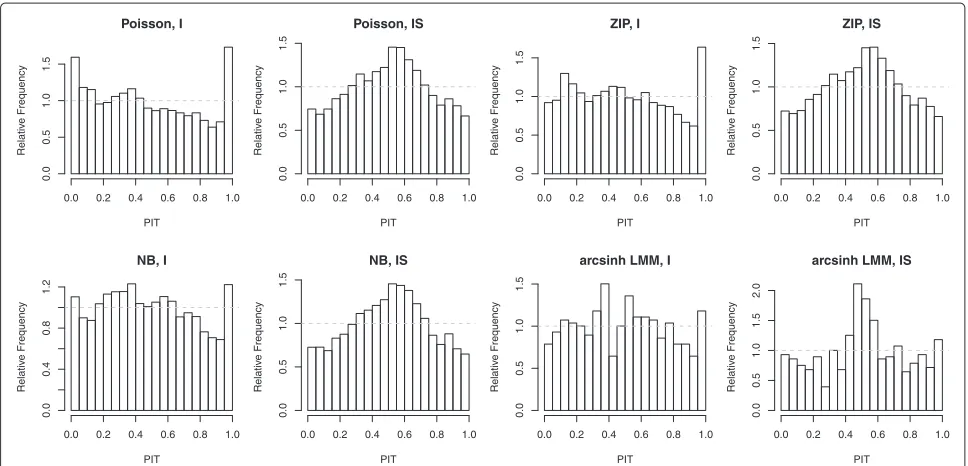
However, our key scientific problem was to quantify the goodness of competing models in terms of prediction
accuracy. The question to be answered was how structural differences concerning random effects or distributional assumptions affect the performance of a posited model. Calibration check was performed by PIT histograms serv-ing as an informal tool for discordancy diagnostics (see Figure 3). In contrast to NB GLMM and arcsinh NMM, which seem to be sufficiently well calibrated for type (I)-models, the Poisson (I) and the ZIP (I) model were slightly U-shaped, indicating a worse predictive performance for
Table 1 INLA summaries for estimated posterior means of population-level parameters (together with 2.5% and 97.5% posterior quantiles) using full Laplace approximations
Parameter Model
Intercept time dosage∗time
Poisson, I 1.366 (1.123, 1.603) -0.051 (-0.063, -0.038) -0.130 (-0.150, -0.109)
Poisson, IS 1.638 (1.432, 1.837) -0.189 (-0.275, -0.107) -0.173 (-0.288, -0.061)
ZIP, I 1.375 (1.121, 1.620) -0.049 (-0.062, -0.036) -0.115 (-0.137, -0.093)
ZIP, IS 1.628 (1.421, 1.830) -0.209 (-0.302, -0.119) -0.198 (-0.323, -0.075)
NB, I 1.447 (1.193, 1.695) -0.069 (-0.090, -0.050) -0.127 (-0.156, -0.098)
NB, IS 1.642 (1.433, 1.840) -0.190 (-0.289, -0.101) -0.168 (-0.289, -0.049)
arcsinh∗, I 2.056 (1.853, 2.259) -0.067 (-0.084, -0.051) -0.074 (-0.096, -0.052)
arcsinh∗, IS 2.055 (1.854, 2.255) -0.068 (-0.114, -0.022) -0.073 (-0.134, -0.012)
Figure 2Vertigo data: INLA vs. MCMC approach.Bayesian inference for fixed effects (Poisson random slope model): comparison of samples from a long MCMC chain () with the posterior marginals computed with the Laplace approximation (—) obtained by using INLA. The vertical blue line shows the posterior mean.
higher columns at the right-hand end of the histograms. Visual assessment of PIT histograms for type (IS)-models revealed noticeable deviations from uniformity due to miscalibration of density forecasts.
Additionally, competing random slope models did not clearly outperform each other. The difference between negative binomial and Poisson was marginal because of a small degree of overdispersion: e.g. the hyperparameter k was estimated to be rather large for the NB (I) model
with random intercepts, with a posterior mean of 7.03, 95% credible interval [ 4.65, 10.36]. For the NB (IS) model, the posterior estimates fork were even larger (data not shown). Likewise, there was no convincing evidence for zero-inflation (e.g. the posterior mean for zero-probability hyperparameterπ0was estimated to be 0.09, 95% credi-ble interval [0.05, 0.14], for ZIP (I). For model type ZIP (IS), the posterior mean forπ0was even less). Modeling the arcsinh-transformed outcome by means of an NMM
Poisson, I
PIT
Relativ
e Frequency
0.0 0.2 0.4 0.6 0.8 1.0
0.0
0.5
1.0
1.5
Poisson, IS
PIT
Relativ
e Frequency
0.0 0.2 0.4 0.6 0.8 1.0
0.0
0.5
1.0
1.5
ZIP, I
PIT
Relativ
e Frequency
0.0 0.2 0.4 0.6 0.8 1.0
0.0
0.5
1.0
1.5
ZIP, IS
PIT
Relativ
e Frequency
0.0 0.2 0.4 0.6 0.8 1.0
0.0
0.5
1.0
1.5
NB, I
PIT
Relativ
e Frequency
0.0 0.2 0.4 0.6 0.8 1.0
0.0
0.4
0.8
1.2
NB, IS
PIT
Relativ
e Frequency
0.0 0.2 0.4 0.6 0.8 1.0
0.0
0.5
1.0
1.5
arcsinh LMM, I
PIT
Relativ
e Frequency
0.0 0.2 0.4 0.6 0.8 1.0
0.0
0.5
1.0
1.5
arcsinh LMM, IS
PIT
Relativ
e Frequency
0.0 0.2 0.4 0.6 0.8 1.0
0.0
0.5
1.0
1.5
2.0
has several computational advantages, and the PIT values seemed reasonably close to uniform for model type (I), hence yielding fairly correct forecasts. Nevertheless, this does not take the sharpness of the density forecasts into account, as opposed to proper scoring rules.
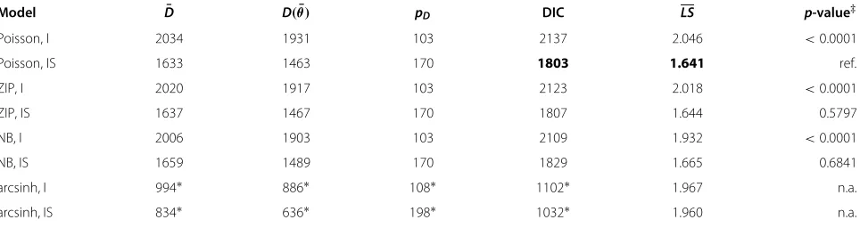
Table 2 enables a comparison of LS and DIC for all eight types of GLMM (the lowest mean score and DIC is printed in bold face). The Poisson (IS) model was ranked best in the leave-one-out predictive assessment by the log-arithmic score. A permutation test was applied to decide whether the difference in mean log scores was signifi-cant on a 5% level. More exactly, we used the Poisson (IS) model emerging with the lowestLSas the reference model and tested in a pairwise manner. The last column of Table 2 depicts Monte Carlop-values based on permu-tation tests (9999 permupermu-tations) for comparison ofLSfor the Poisson (IS) GLMM withLSif the remaining compet-ing models are chosen for data analysis. n.a. means that a permutation test is not applicable because of backtrans-formation ofLSobtained within the arcsinh-NMM (see Appendix A2 for further details).
The Poisson (IS) model and the negative binomial (IS) counterpart do not differ significantly with respect to their mean cross-validated logarithmic scores. The same holds for the ZIP (IS) alternative. Ranking these models by means of their DIC value (disregarding NMM types) revealed that they are very close to each other.
In summary, there was no evidence of considerable over-dispersion and excess of zeros. Inclusion of a zero-inflation component is apparently not necessary for these pre-study data. Applying mean log score and DIC to rank all eight models considered so far suggests that random intercept models are inferior to random intercept and slope models.
Hence, we are inclined to believe that a Poisson random intercept and slope model is suitable for these longitudinal count response data.
SAP for BEMED trial: selection of candidate models
After detailed analyses of the pre-study data described above, we will present these results in the SAP and choose a negative binomial model with random intercepts as well as random slopes as a robust candidate to conduct sensitivity analyses for the efficacy data of the BEMED trial. Accordingly, this proposed modeling strategy will be determined in the SAP.
Simulation study Sampling details
In the last section, a prediction-oriented Bayesian toolbox was applied to real-life clinical count data. It is also impor-tant to investigate whether these tools help to evaluate different model alternatives and whether the model com-parisons are valid. To assess the discriminatory power as well as the properties of DIC and mean logarithmic score in the longitudinal count response situation, a simulation study was carried out. Following the real data structure of our clinical trial about patients with vertigo attacks, a par-allel group design was assumed with four measurements occurring at timest = (t1,t2,t3,t4) = 0, 1, 2, 3 (exactly balanced design) for all subjects. There are two groups each of sizen, with different fixed time slopes, parame-terized byβ1 = −0.3 andβ2 = −0.5, but equal starting points at timet1=0. To be more detailed, we considered repeated count outcomes to follow a negative binomial distribution, conditioned on the random effects. Accord-ingly, the true sampling model is Yij|μi ∼iid NB(k,pi),
i=1,. . ., 2n,j=1,. . ., 4. To account for patient-specific variability, a random interceptai was introduced, so the
model can be summarized as
logμij=α+ai+tij[β2Gi+β1(1−Gi)] ,
withai|σa−2 ∼N(0,σa2), andGirepresenting the placebo
and the verum group, respectively. The standard deviation
Table 2 Posterior mean of the deviance (D¯), deviance of the mean (D(θ)¯ ), effective number of parameters (pD) as measure
of model complexity, DIC value, and mean of logarithmic scores (LS)
Model D¯ D(θ)¯ pD DIC LS p-value‡
Poisson, I 2034 1931 103 2137 2.046 <0.0001
Poisson, IS 1633 1463 170 1803 1.641 ref.
ZIP, I 2020 1917 103 2123 2.018 <0.0001
ZIP, IS 1637 1467 170 1807 1.644 0.5797
NB, I 2006 1903 103 2109 1.932 <0.0001
NB, IS 1659 1489 170 1829 1.665 0.6841
arcsinh, I 994∗ 886∗ 108∗ 1102∗ 1.967 n.a.
arcsinh, IS 834∗ 636∗ 198∗ 1032∗ 1.960 n.a.
∗Comparison of DIC for NMMs is not applicable because of differentarcsinh-transformed outcomes.
of the random intercept was set to σa = 0.3 and the
population intercept fixed atα = 3. The following candi-date GLMMs are ranked by DIC as well as evaluated with respect to their forecasting capability:
• negative binomial (true data generating distribution),
• Poisson,
• zero-inflated Poisson,
• zero-inflated negative binomial,
• NMM for arcsinh-transformed count outcome.
The ZIP and ZINB model were chosen to investigate whether the zero-inflated component improves the model performance. To define simulation scenarios we varied the sampling size (n, numbers per group) and the degree of over-dispersion as follows: n = 20, 50, 100 and k = 0.5, 1, 5, 10, 20, 50. By combining the possible values of the sample size and the overdispersion parameterk, we therefore obtain count data for 18 different simulation scenarios which can be analyzed for all five rival models described above. Each model scenario providedr = 100 simulation runs to assess the variability of results.
All analyses were performed using the INLA approach. To get reliable results and to enhance the accuracy of Bayesian predictive measures (i.e. DIC and logarithmic CPO values), the full Laplace approximation in combi-nation with the so-called GRID integration scheme was chosen as the strategy for deterministic approximation of the latent Gaussian field and the posterior marginals of the hyperparameters. For more details of estimation pro-cedure, the reader is referred to [37,51] and the Additional files 1 and 2 (Supplementary Material).
When working with small data sets, the prior distri-bution can become influential in the posterior results, especially with respect to the spread of the posterior dis-tribution, even if non-informative settings are chosen. This can particularly be an issue with prior distributions on the variance components. Therefore, for prior spec-ification we followed the procedure outlined in [40] so as not to favor one modeling strategy over another. We assumed a marginal Cauchy distribution for the patient-specific intercept ai. A 95% range of [−0.6, 0.6] for ai
gives a prior σa−2 ∼ Ga(0.5, 0.001115), and hence, inte-gration overσa−2gives the marginal distribution ofaias
t1(0, 0.00223, 1).
Simulation results
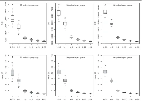
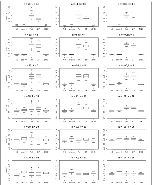
Figure 4 depicts boxplots for different simulation sce-narios if count response data {y(ijr)}, i = 1,. . ., 2n; j = 1,. . ., 4;r = 1,. . ., 100, are analyzed by choosing a Pois-son GLMM, i.e. a wrong modeling strategy in the case of high overdispersion. Both DIC as a measure of model selection and mean of logarithmic score (LS(r), r = 1,. . ., 100) were calculated for all 100 runs. The striking
feature of these plots is that for all 6 setups, DIC andLS discriminate strongly between the wrong model and the true negative binomial model generating the counts. If a Poisson model is chosen for data with a considerably high amount of overdispersion (small k), higher score values are assigned to the predictive distribution. DIC is clearly influenced by the sample size because of the deviance measure depending on the likelihood, whereas forLSthe number of sampling units does not impact scaling of the mean of the scores.
Based on these simulations, we conclude that DIC and LSprovide a suitable measure for ranking and evaluating model alternatives defined by different error distributions or variance structures.
For all three sample size situations (i.e. 40, 100, 200 units in total), Figure 5 reveals the difference in mean log scores for the true negative binomial GLMM compared with the following model alternatives: Poisson (neglect-ing over-dispersion), zero-inflation (assum(neglect-ing an excess of zeros) and a Gaussian response model after arcsinh-transformation of the counts yij. The inadequacy of the
Poisson model in terms of probabilistic forecasting is evi-dent in the case of high overdispersion, denoted by the parameterk. Ifk→ ∞,LSof the “wrong” Poisson model approximates the mean log score of the true NB model.
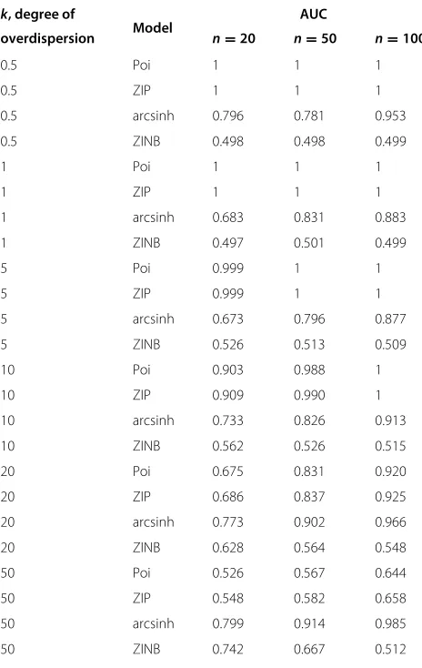
Furthermore, Table 3 reports the area underneath the receiver operating curve (AUC) as a summary measure for LS(r), r = 1,. . ., 100, of the true NB model and a competing model alternative, as displayed in Figure 5. For each combination ofk(degree of overdispersion) and n (sample size) the discriminatory power of the mean log score was investigated. Perfect discrimination corre-sponds to an AUC value of 1 while random discrimination corresponds to an AUC value of 0.5. The AUC can be interpreted as being equal to the probability that LS of the wrong model exceeds that of the true NB model, i.e. the probability that the wrong model has a lower predic-tive performance compared with the true data generating distribution. Accordingly, it is the probability that test results from a randomly selected pair ofLS(r) values for the wrong model and the true NB model are correctly ordered, namely Pr(LS(r,wrong)>LS(r,true)),r=r.
Figure 4Simulation study: Discriminatory power of DIC andLSfor different scenarios (100 runs per scenario).Data generating process: longitudinal, negative binomial counts with subject-specific intercept (balanced design); modeling strategy: Poisson GLMM with random intercept; number of subjects per group:n=20, 50, 100; degree of overdispersion:k=0.5, 1, 5, 10, 20, 50. Ask→ ∞, the degree of overdispersion decreases and the negative binomial converges to a Poisson distribution. Hence, DIC andLSdecline. Note that the range of DIC increases in the case of a larger sample size.
arcsinh NMM as an alternative to accomplish variance-stabilization, the AUC is lower than that of a wrong Poisson model. However, if k → ∞ and the amount of overdispersion goes down, the choice of an NMM for arcsinh-transformed counts results in AUC clearly larger than 0.5. Hence, the quality of observation-level predic-tions of the NMM is worse than that of the (zero-inflated) Poisson. If the negative binomial converges in distribution to the Poisson, the arcsinh-transformation of the count outcome is no longer appropriate.
Discussion
We have discussed Bayesian strategies for model evalu-ation of GLMMs for longitudinal count data and used integrated nested Laplace approximations to do the cal-culations. We especially looked at tools such as the DIC, logarithmic score, and PIT. These techniques for model assessment are implemented in the package R-INLA
which can easily be used inRand aim to score the mod-els with respect to their appropriateness explaining the observed data. Therefore, a very practical toolbox is at the hand for statisticians. It must be noted that other instru-ments such as pivotal quantities [71] or different proper scoring rules [28] can be used if the calculations are done with MCMC methods (e.g. using WinBUGS [55,72]).
Table 3 Area under the curve (AUC) for comparison of
mean logarithmic scoreLS(r)of true vs. wrong modeling
strategy (r=1,. . ., 100 iterations per simulation scenario)
k, degree of AUC
overdispersion Model n=20 n=50 n=100
0.5 Poi 1 1 1
0.5 ZIP 1 1 1
0.5 arcsinh 0.796 0.781 0.953
0.5 ZINB 0.498 0.498 0.499
1 Poi 1 1 1
1 ZIP 1 1 1
1 arcsinh 0.683 0.831 0.883
1 ZINB 0.497 0.501 0.499
5 Poi 0.999 1 1
5 ZIP 0.999 1 1
5 arcsinh 0.673 0.796 0.877
5 ZINB 0.526 0.513 0.509
10 Poi 0.903 0.988 1
10 ZIP 0.909 0.990 1
10 arcsinh 0.733 0.826 0.913
10 ZINB 0.562 0.526 0.515
20 Poi 0.675 0.831 0.920
20 ZIP 0.686 0.837 0.925
20 arcsinh 0.773 0.902 0.966
20 ZINB 0.628 0.564 0.548
50 Poi 0.526 0.567 0.644
50 ZIP 0.548 0.582 0.658
50 arcsinh 0.799 0.914 0.985
50 ZINB 0.742 0.667 0.512
True model: negative binomial GLMM; competing modeling strategies: Poisson, ZIP, NMM for arcsinh-transformed counts, ZINB. Sample size: n=20, 50, 100 patients per group; degree of overdispersion:k=0.5, 1, 5, 10, 20, 50. AUC can be interpreted as a summary measure for the goodness of discrimination between the true negative binomial model generating the longitudinal data and rival models which should be taken into consideration in practice. Fork→ ∞, the difference between a negative binomial and the alternative Poisson model dissolves because of convergence in distribution; therefore, AUC→0.5 and both model alternatives approximate with respect to their forecasting ability.
We next discuss four important aspects of this pro-cess: prior distributions, normality assumption for ran-dom effects, Bayesian model evaluation, and modeling of clinical trial data.
Prior distributions
Bayesian analysis needs a specification of prior distri-butions. However, when fitting a GLMM in a Bayesian setting, specifying prior distributions is not straightfor-ward; this is particularly true for variance components. Fonget al. [40] pointed out that the priors for variance
components should be chosen carefully. To quantify the sensitivity of the posterior distributions with respect to changes in the priors for the random effects precision parameters, Roos & Held [73] discuss a measure based on the so-called Hellinger distance for GLMMs with binary outcome but not for count data. Adapting their approach to count data is a topic for future research. In this study, we followed advice from the literature: in the case of neg-ative binomial models, estimation of the posterior mean of the dispersion parameter can be affected when a vague prior specification is used to characterize the gamma hyper-parameter. To circumvent the problem of distort-ing posterior inferences, e.g. Lordet al.[74] recommend a non-vague prior distribution for the dispersion parame-ter to minimize the risk of a mis-estimated posparame-terior mean and to obtain stable and valid results. This issue is par-ticularly relevant for data characterized by a small sample size in combination with low sample mean values. The situation is quite complex and the only practical way to handle this issue is a careful simulation study to investi-gate whether changing priors would influence the decision on the relevant model. The material provided in the Web Supplement may help a statistician set up such simulation studies.
Gaussian random effects