HYPOTHESIS TESTING FOR AN EXCHANGEABLE NORMAL
DISTRIBUTION
A. Mohammadpour
1and J. Behboodian
2*1
Department of Statistics, Faculty of Mathematics & Computer Science, Amirkabir University of Technology, Tehran 15914, Islamic Republic of Iran
2
Department of Statistics, College of Sciences, Shiraz University, Shiraz 71454, Islamic Republic of Iran
Abstract
Consider an exchangeable normal vector with parameters
μ
,
σ
2, and
ρ
. On the
basis of a vector observation some tests about these parameters are found and their
properties are discussed. A simulation study for these tests and a few
nonparametric tests are presented. Some advantages and disadvantages of these
tests are discussed and a few applications are given.
*
E-mail: [email protected] 1. Introduction
Statistical studies are often based on independent and identically distributed (IID) random variables. In applications we may not have such strong assumptions on the observations. A weaker assumption is exchangeability. Exchangeable random variables were first introduced by de Finetti [5] and then considered by many researchers, for example, Chow & Teicker [4], de Finetti [6,7,8], Feller [10], Fürst [12], and Koch & Spizzichino [14].
This work is concerned with hypothesis testing for an exchangeable normal distribution. The random vector
X=(X1,…, Xp)´ is said to have an exchangeable normal distribution if its distribution is multivariate normal with the following mean vector and variance-covariance matrix
). 1 , 0 [ , 0 ,
1 1 1
, ,
.
2
1
∈ > ⎟ ⎟ ⎟
⎠ ⎞
⎜ ⎜ ⎜
⎝ ⎛
⋅ ⋅ ⋅ ∞ < < ∞ − ⎟ ⎟ ⎟
⎠ ⎞
⎜ ⎜ ⎜
⎝ ⎛
× ×
ρ σ ρ
ρ ρ
ρρ ρ
σ μ μ
μ μ
p p
p K
K K K
Keywords: Exchangeable normal distribution; Power func-tion; Robust test; Test of randomness; Uniformly most power-ful test; Uniformly most powerpower-ful unbiased test
(see, e.g., Tong [21], page 112). We denote this exchangeable normal distribution with three parameters
μ, σ2
, and ρ by ENp(μ, σ2, ρ). It is clear that (X1,…, Xp) and (X , , X )
p
i
i1… are identical in distribution for any
permutation {i1,…,ip} of {1,…,p}.
Some statisticians have worked on this distribution. For example, Rao [19] has a t-test for μ, McElroy [17] considers a regression study with exchangeable normal errors, and Arnold [1] extends this study to linear models.
In Section 2, we study some tests about the parameters of an exchangeable normal distribution, and we plot their power functions. Section 3 is concerned with a simulation study and a comparison of these tests with a few nonparametric tests. In Section 4 a few applications are given for these tests.
2. Hypothesis Testing
In this section we introduce some intuitively test functions for testing the parameters of an exchangeable normal vector X. We also point out some restrictions on these tests and find the best ones.
First we study two tests for ρ. Suppose we want to
test , when μ is known. It can be proved that
⎩ ⎨ ⎧
> =
0 :
0 :
1 0
ρ ρ
1 ) 1 ( 1 ) 1 ( / + − = − − − p T p p S X ρ ρ μ ,
where = denotes equality in distribution, X and S2
denotes the sample mean and variance respectively, and
Tp-1 denotes the t-variable with p-1 degrees of freedom
(see Rao [19] page 197). Under H0:ρ=0, we have
1
/ =T −
−
p
p S
X μ
. If ρ is close to 1 then
ρ ρ ) 1 ( 1 ) 1 ( − + −
p is
close to 0. Therefore, we reject H0 if 1or 2
/ p k k s x > −μ , where 2 1 , 1 1= − −α
p
t
k , and k2= -k1, and P(Tp−1>
2 ) 2 1 , 1 α α = − − p t .
Now, consider the case that σ 2 is known but μ is unknown. It can be proved that
2 1 2 2 ) 1 ( ) 1 ( − = − − p S p χ σ ρ ,
where denotes the chi-square distribution with p-1
degrees of freedom (see Rao [19] page 197). Under , we have . If ρ is close
to 1 then (1-ρ) is close to 0. Thus, we reject H
2 1 − p χ 0 :
0 ρ=
H (p−1)S2/σ2=χ2p−1
0, if , where
. 2 , 1 2 2 / ) 1
(p− s σ <χp− α
α χ
σ α
ρ= (( −1) / < 2−1, )= 2
2
0 p S p
P
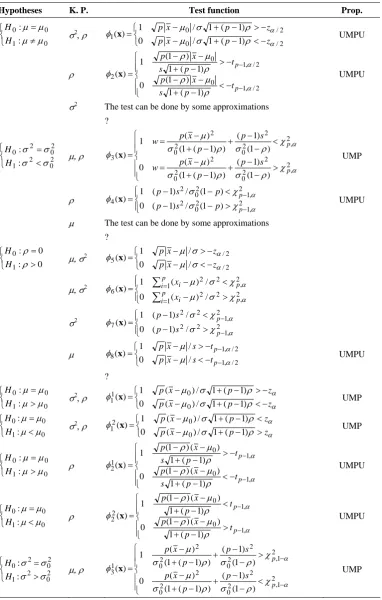
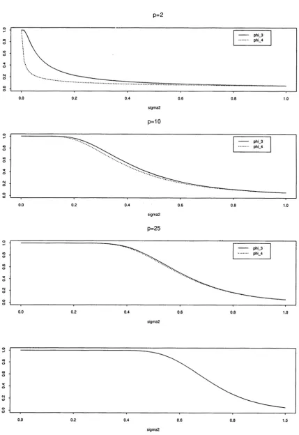
Table 1 shows intuitively test functions for parameters of an exchangeable normal vector and Figures 1-4 show their power functions (the graphs and the computations are prepared by S-PLUS). We use the following abbreviation in this table, K: known, P: parameter, Prop: property, UMP: uniformly most powerful, UMPU: UMP unbiased.
Note that, there is no test for anyone of μ, σ 2, and ρ, when two of them are unknown. A main reason for this, due to the fact that dimension of minimal sufficient statistic is less than the dimension of parameter space (see Remark 2.1).
In the following theorem we prove that some of the test functions in Table 1 are the best.
Theorem 2.1. If X=(X1,…, Xp)´ has the distribution
ENp(μ, σ2, ρ), then the test functions in Table 1 follows the properties in the last column of this table.
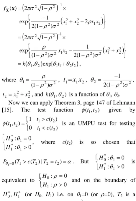
Proof. Hypothesis testing for ρ. Let μ be known. Without loss of generally assume that μ =0. First consider the case p=2. In this case the joint density of
X=(X1, X2)´ is given by
(
)
(
)
(
)
(
)
(
,)
exp{
}
,) 1 ( 2 1 ) 1 ( exp 1 2 2 ) 1 ( 2 1 exp 1 2 ) ( 2 2 1 1 2 1 2 2 2 1 2 2 2 1 2 2 1 2 2 2 1 2 2 2 1 2 2 1 2 2 t t k x x x x x x x x f θ θ θ θ σ ρ σ ρ ρ ρ πσ ρ σ ρ ρ πσ + = ⎭ ⎬ ⎫ ⎩ ⎨ ⎧ + − − − × − = ⎭ ⎬ ⎫ ⎩ ⎨ ⎧ + − − − × − = − − x X d d d
where 1 2 2
) 1 ( ρ σ
ρ θ
−
= ,
t
1=
x
1x
2, ,) 1 ( 2 1 2 2 2 σ ρ θ − − =
, and is a function of θ
2 2 2 1 2 x x
t = + k(θ1,θ2) 1, θ2.
Now we can apply Theorem 3, page 147 of Lehmann [15]. The test function given by
is an UMPU test for testing
, where c(t
) , (t1 t2
φ ⎩ ⎨ ⎧ < > = ) ( 0 ) ( 1 ) , ( 2 1 2 1 2 1 t c t t c t t t φ ⎩ ⎨ ⎧ > = 0 : 0 : 1 * 1 1 * 0 θ θ H H
2) is so chosen that
α θ1=0(T1>c(T2)|T2=t2)=
P . But is
equivalent to and on the boundary of
(or H
⎩ ⎨ ⎧ > = 0 : 0 : 1 * 1 1 * 0 θ θ H H ⎩ ⎨ ⎧ > = 0 : 0 : 1 0 ρ ρ H H * 1 * 0,H
H 0, H1) i.e. on θ1=0 (or ρ=0), T2 is a
complete sufficient statistic for σ 2. If we define
d d , ) ( 2 2 2 2 2 2 1 2 2 1 2 2 2 1 2 2 1 2 2 2 1 2 2 2 1 2 1 2 2 1 σ σ σ X X X X X X X X X X X X X X T T T T + ⎟ ⎠ ⎞ ⎜ ⎝ ⎛ + = + + = + + + = + = ′
then T´ is an ancillary and as a result independent from
T2. Therefore,
, ) ( ) | ) ( ( ) | ) ( ( 2 0 2 2 2 1 0 2 2 2 1 0 1 1 1 c T P t T T c T P t T T c T P > ′ = = > ′ = = > = = = θ θ θ where 2 2 2 2 1 ) ( 2 ) ( T T T c T
c = + and is a
constant to be determined for a given α. Hence,
) (2
1 2 c t
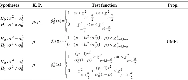
Table 1. Intuitively test functions for hypothesis testing for an ENp(μ, σ2, ρ)
Hypotheses K. P. Test function Prop.
⎩ ⎨ ⎧ ≠ = 0 1 0 0 : : μ μ μ μ H H
σ2, ρ
⎩ ⎨ ⎧ − < − + − − > − + − = 2 / 0 2 / 0 1 ) 1 ( 1 / 0 ) 1 ( 1 / 1 ) ( α α ρ σ μ ρ σ μ φ z p x p z p x p x UMPU ρ ⎪ ⎪ ⎩ ⎪⎪ ⎨ ⎧ − < − + − − − > − + − − = − − 2 / , 1 0 2 / , 1 0 2 ) 1 ( 1 ) 1 ( 0 ) 1 ( 1 ) 1 ( 1 ) ( α α ρ μ ρ ρ μ ρ φ p p t p s x p t p s x p x UMPU
σ2 The test can be done by some approximations
?
⎩H1:σ <σ0
⎨ ⎧ = 2 2 2 0 2 0:σ σ
H μ, ρ ⎪ ⎪ ⎩ ⎪ ⎪ ⎨ ⎧ > − − + − + − = < − − + − + − = = 2 , 2 0 2 2 0 2 2 , 2 0 2 2 0 2 3 ) 1 ( ) 1 ( ) ) 1 ( 1 ( ) ( 0 ) 1 ( ) 1 ( ) ) 1 ( 1 ( ) ( 1 ) ( α α χ ρ σ ρ σ μ χ ρ σ ρ σ μ φ p p s p p x p w s p p x p w x UMP ρ ⎪⎩ ⎪ ⎨ ⎧ > − − < − − = − − 2 , 1 2 0 2 2 , 1 2 0 2 4 ) 1 ( / ) 1 ( 0 ) 1 ( / ) 1 ( 1 ) ( α α χ σ χ σ φ p p p s p p s p x UMPU
μ The test can be done by some approximations
? ⎩ ⎨ ⎧ > = 0 : 0 : 1 0 ρ ρ H H
μ, σ2
⎩ ⎨ ⎧ − < − − > − = 2 / 2 / 5 / 0 / 1 ) ( α α σ μ σ μ φ z x p z x p x
μ, σ2
⎪⎩ ⎪ ⎨ ⎧ > − < − =
∑
∑
= = 2 , 1 2 2 2 , 1 2 2 6 / ) ( 0 / ) ( 1 ) ( α α χ σ μ χ σ μ φ p p i i p p i i x x x σ2 ⎪⎩ ⎪ ⎨ ⎧ > − < − = − − 2 , 1 2 2 2 , 1 2 2 7 / ) 1 ( 0 / ) 1 ( 1 ) ( α α χ σ χ σ φ p p s p s p x μ ⎩ ⎨ ⎧ − < − − > − = − − 2 / , 1 2 / , 18 0 /
/ 1 ) ( α α μ μ φ p p t s x p t s x p x UMPU ? ⎩ ⎨ ⎧ > = 0 1 0 0 : : μ μ μ μ H H
σ2, ρ
⎩ ⎨ ⎧ − < − + − − > − + − = α α ρ σ μ ρ σ μ φ z p x p z p x p ) 1 ( 1 / ) ( 0 ) 1 ( 1 / ) ( 1 ) ( 0 0 1
1 x UMP
⎩ ⎨ ⎧ < = 0 1 0 0 : : μ μ μ μ H H
σ2, ρ
⎩ ⎨ ⎧ > − + − < − + − = α α ρ σ μ ρ σ μ φ z p x p z p x p ) 1 ( 1 / ) ( 0 ) 1 ( 1 / ) ( 1 ) ( 0 0 2
1 x UMP
⎩ ⎨ ⎧ > = 0 0 : : μ μ μ μ H H 0 1 ρ ⎪ ⎪ ⎩ ⎪⎪ ⎨ ⎧ − < − + − − − > − + − − = − − α α ρ μ ρ ρ μ ρ φ , 1 0 , 1 0 1 2 ) 1 ( 1 ) ( ) 1 ( 0 ) 1 ( 1 ) ( ) 1 ( 1 ) ( p p t p s x p t p s x p x UMPU ⎩ ⎨ ⎧ < = 0 0 : : μ μ μ μ H H 0 1 ρ ⎪ ⎪ ⎩ ⎪⎪ ⎨ ⎧ > − + − − < − + − − = − − α α ρ μ ρ ρ μ ρ φ , 1 0 , 1 0 2 2 ) 1 ( 1 ) ( ) 1 ( 0 ) 1 ( 1 ) ( ) 1 ( 1 ) ( p p t p x p t p x p x UMPU
⎩H1:σ >σ0 ⎨ ⎧ = 2 2 2 0 2 0:σ σ
Table 1. Continued
Hypotheses K. P. Test function Prop.
⎩ ⎨ ⎧ ≠ = 2 2 2 0 2 0 : : σ σ σ σ H H 0 1 μ, ρ ⎪ ⎪ ⎩ ⎪⎪ ⎨ ⎧ < < < > = − − 2 2 1 , 2 2 , 2 2 , 2 2 1 , 2 3 0 or , 1 ) ( α α α α χ χ χ χ φ p p p p w w x ⎩ ⎨ ⎧ > = 2 0 2 1 2 0 2 0 : : σ σ σ σ H H ρ ⎪⎩ ⎪ ⎨ ⎧ < − − > − − = − − − − 2 1 , 1 2 0 2 2 1 , 1 2 0 2 1
4 0 ( 1) / (1 )
) 1 ( / ) 1 ( 1 ) ( α α χ ρ σ χ ρ σ φ p p s p s p x UMPU
⎩ ≠ 2
0 2 1:σ σ
H
⎨
⎧ = 2
0 2 0:σ σ
H ρ ⎪ ⎪ ⎩ ⎪ ⎪ ⎨ ⎧ < − − < < > − − = − − − − − − 2 2 1 , 1 2 0 2 2 2 , 1 2 2 , 1 2 2 1 , 1 2 0 2 2 4 ) 1 ( ) 1 ( 0 or , ) 1 ( ) 1 ( 1 ) ( α α α α χ ρ σ χ χ χ ρ σ φ p p p p s p s p x
where c2 may be chosen so that Pθ1=0(T′>c2)=α. In
fact, this test is the usual t-test, more often written in the form of ⎪ ⎪ ⎩ ⎪⎪ ⎨ ⎧ ′ < ′ > = , / 0 / 1 ) x ( c p s x c p s x φ
where p=2,
p t t
x = 21+ 2 , =
∑
− − ==( ) /( 1)
2 1 2 p x x
s ip i
) 1 /( )
(t2−px2 p− (see Ferguson [11] page 230). With
) 2 1 ; 1 ( − −α
=
′ t p
c , the test function is an UMPU
size-α test for testing ⎨⎧ .
) (x φ ⎩ > = 0 : 0 : 1 0 ρ ρ H H
When p>2, the proof is similar to the above proof. In this case, by some simple algebraic calculations or using an orthogonal transformation we can show that the density of X=(X1,…, Xp)´ is
(
)
(
)
, ) 1 ( 2 ) 1 )( ) 1 ( 1 ( 2 exp ) , ( ) 1 )( ) 1 ( 1 ( ) 1 ( 2 1 exp ) , ( ) ( 2 1 2 2 2 2 2 2 1 2 1 2 2 ⎪⎭ ⎪ ⎬ ⎫ − − ⎪⎩ ⎪ ⎨ ⎧ − − + = ⎪⎭ ⎪ ⎬ ⎫ ⎥ ⎥ ⎦ ⎤ − − + − ⎪⎩ ⎪ ⎨ ⎧ ⎢ ⎢ ⎣ ⎡ − − =∑
∑
∑
= = = ρ σ ρ ρ σ ρ σ ρ ρ ρ σ ρ ρ σ σ ρ p i i p p i i p i i p x p x p p k p x x kfX x
where 2 / 1 2 / ) 1 ( 2 ) ) 1 ( 1 ( ) 1 ( ) 2 ( ) ,
(ρ σ = πσ − −p − − + p− ρ −
kp p p
(see Tong [21] page 112, formula (5.3.8)´ which contains an error). Note that,
p x x x x p p i i j
i i j )/
2 ( ) ( 1 2
2
∑
∑
= < + = . Therefore, } , exp{ ) , ( )
( k 1 2 1t1 2t2
fX x = ′p θ θ θ θ , (2.1)
where θ1=ρ/(σ2(1+(p−1)ρ)(1−ρ)), =
∑
<j i xixj
t1 ,
,
∑
== p
i xi
t2 1 2 k′p(θ1,θ2) is a function of θ1, θ2, and θ2
can be determined. The rest of this case is similar to the case p=2. Therefore, φ8 is UMPU.
Hypothesis Testing for μ. Note that X and (X,S2) are minimal sufficient statistics for μ and (μ, σ 2) when (σ 2, ρ) are known, respectively. It is known that
) / ) ) 1 ( 1 ( ,
( p p
N
X= μ + − ρ , and
are independent. Therefore, the properties of the
tests , , , , and can be proved immediately (see e.g., Lehmann [15] page 192).
= −
−1) /((1 ) )
(p S2 ρ σ2
2 1 − p χ 1 φ 1 1 φ 2 1
φ φ2 1
2
φ 2
2
φ
d d
Hypothesis Testing for σ 2
. Let (μ, ρ) be known. Fix σ 2 under H1 and apply the Neyman-Pearson lemma (see
also Hypothesis testing for ρ). Then we have the properties of , and . The proof for the properties of
, and is similar to the test functions of μ.
3 φ 1 3 φ 4 φ 1 4 φ
Remark 2.1. If μ and σ2 are both unknown we have trivial UMPU test for ρ. To prove this fact we observe that
{11 22 33}
3 2 1, , )exp
( )
( q t t t
fX x = p θ θ θ θ +θ +θ ,
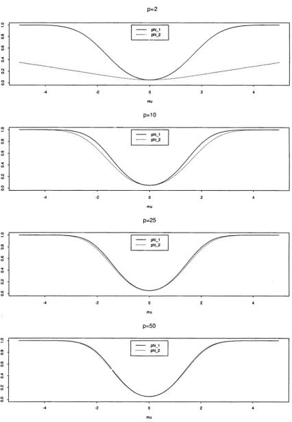
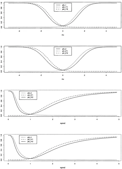
Figure 4. Power functions for the tests φ1, φ11, and φ12; φ2, φ21, and φ22; φ3, φ31, and φ32; and φ4, φ41, and φ42, where
l
/
1 ρ
θ = , , ,
, , ,
, and
∑
<= i jxixj
t1 θ2=−(1+(p−2)ρ)/(2l)
∑
== p
i xi
t2 1 2 θ3=(1−ρ)μ/l t3=
∑
ip=1xi l=σ2(1+ )1 )( ) 1
(p− ρ −ρ qp(θ1,θ2,θ3) can be determined.
Therefore the test function given by
is a UMPU test for
testing where is so chosen that
) , (t1 t2
φ
=
) , , (t1 t2 t3
φ
⎩ ⎨ ⎧
< >
) ( 0
) ( 1
3 , 2 1
3 , 2 1
t t c t
t t c t
⎩ ⎨ ⎧
> =
0 :
0 :
1 0
ρ ρ
H H
) , (t2 t3 c
α θ1=0(T1>c(T2,T3)|T2 =t2,T3 =t3)=
P .
Note that and also the event
depends on T
2 / ) ( 32 2
1 T T
T = −
)} , (
{T1>cT2 T3 2 and T3. Therefore, we
have
⎩ ⎨ ⎧
< > =
= = >
= 0 ( )
) ( 1
) , | ) , ( (
3 , 2 1
3 , 2 1 3
3 2 2 3 2 1 0
1 t ct t
t t c t t
T t T T T c T
Pθ ,
which is equal to . If we use the method in the proof of Theorem 2.1, then we obtain a similar result.
) , , (t1 t2 t3
φ
Remark 2.2. If σ2 is known but μ is unknown, we cannot have such an UMPU test for ρ by the method given in Theorem 2.1, because the density is not of the form (2.1).
Remark 2.3. As in the case ρ = 0, the test is not UMP.
1
φ
Remark 2.4. The tests , and are not UMP or UMPU, because when ρ = 0 they are not UMP or UMPU (see Tate & Klett [20], and Parsian & Nematolahi [18]).
2 3
φ 2
4
φ
Remark 2.5. The tests and are not UMPU. To show this fact, compare these tests with in Figure 3.
5
φ φ6
8
φ
3. A Simulation Study
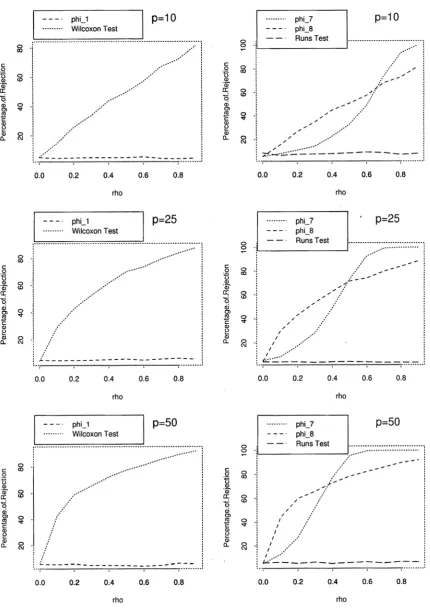
In this section we consider the effect of ρ > 0 on the test functions in Section 2. For this purpose we change ρ in the interval [0,1) and by simulation we study the robustness of these test functions. A good test function for μ or σ 2 should be robust when ρ changes in [0,1), but not for testing ρ.
For example, consider , the test function for testing
, when , and α = 0.05. Figure 5
(left column) shows the percentage times of rejecting H
1
φ
⎩ ⎨ ⎧
≠ =
0 1
0 0
: :
μ μ
μ μ
H H
0
0 =
μ
0
when μ = 0 for . This test is robust, because percentage times of rejecting H
) 1 , 0 [
∈ ρ
0 are approximately 5%
for all . But, for example, the Wilcoxon test (nonparametric test for mean; see, e.g., Gibbons [13]) is not robust, i.e. percentage times of rejecting H
) 1 , 0 [
∈ ρ
0
increases when ρ goes to 1.
However tests for ρ should not be robust, because they are sensitive to the change of ρ. Now consider , and the Runs test (test of randomness; see, e.g., Gibbons [13]). Figure 5 (right column) shows the percentage times of rejecting H
7
φ
8
φ
0. At ρ = 0, the
percentage times of rejecting H0 for these tests are
approximately 5%. When ρ increases the percentage goes up for φ7 and φ8, but not for the Runs test.
Remark 3.1. To simulate an ENp(μ, σ 2, ρ), we use the Algorithm 8.1.2 of Tong [21] page 183, by an S-PLUS function. We generate 2000 times from an ENp(0, 1, ρ) for ρ = 0, 0.1,…, 0.9. The complete result of this simulation can be downloaded from the author’s homepage on the World Wide Web.
4. Applications
The main result of the previous section was the advantage of the following tests ,…, , and . In this section, we try to answer the following question:
1
φ φ4 φ7 φ8
Can we use the test functions ,…, , , and in applied problems?
1
φ φ4 φ7
8
φ
Suppose we have the assumption of normality. Consider the test functions , and . These test functions are useful if the parameter ρ is known, but in a real problem ρ is usually unknown and there is no estimate or nontrivial test for ρ. Therefore, we cannot test for μ or σ
2
φ φ4
2
, unless ρ is known. Note that if μ or σ2 is known then we can estimate ρ and there is a test for ρ ( , or ), and so the tests , and are applied for testing μ, and σ
7
φ φ8 φ1 φ3
2
, respectively after applying the test , or .
7
φ
8
φ
In the following, we point out some difficulties and restrictions for using tests φ7, and φ8.
Linear Models
The error terms in linear models usually have IID normal distribution with zero mean and unknown variance σ 2. One of the important problems in linear models is checking the assumption of IID or ρ = 0. Unfortunately, we cannot use test , because the sum of estimated errors is zero (see Arnold [1]).
8
φ
Time Series
zero, so we can check the assumption of independence. Note that if we subtract the mean of observations from them (this transformation is usually used in time series, see, e.g., [2,3]) then the mean of estimated errors is near zero, so we cannot use test . Dufour and Roy [9] introduce some tests for checking independence assumption in exchangeable time series.
8
φ
Statistical Quality Control
Suppose a process is generated by a system. If we cannot reject the assumption of normality then we can use the test functions , and , when variance or mean of the system is known, respectively. For an application of these tests see Section 7.2.1 of Leitnaker, Sanders and Hild [16].
7
φ φ8
Acknowledgements
The authors would like to thank the referees for their helpful comments. They are also grateful to the Shiraz University Research Council for supporting this work.
References
1. Arnold, S. F. Linear models with exchangeably distri-buted errors. Journal of the American Statistical Asso-ciation, 74, 194-199, (1979).
2. Brockwell, P. J. and Davis, R. A. Time Series: Theory and Methods. Springer-Verlag, Berlin Heidelberg New York, pp. 306-314, (1991).
3. Brockwell, P. J. and Davis, R. A. ITSM for Windows: User’s Guide to Time Series Modeling and Forecasting.
Springer-Verlag, Berlin Heidelberg New York, pp. 36-42, (1991).
4. Chow, Y. S. and Teicker, H. Probability Theory. (2nd ed.), Springer-Verlag, New York, 182, 220-226, (1987). 5. de Finetti, B. Funzione carattenisbica di un fenomeno
aleatorio. Memorie R. Accad. Lincei, 4(5), 86-133, (1930).
6. de Finetti, B. Teoria della probabilita. Einaudi, Torino, (1970). (English Translation, Theory of probability, Vol. II, Wiley, New York, pp. 211-224, (1974-75).)
7. de Finetti, B. Probability, Induction, and Statistics.
Wiley, New York, Vol. 8, p. 160, (1972).
8. de Finetti, B. Foresigh: Its logical law its subjective sources. Breakthroughs in Statistics Vol. I, Kotz, S. and Johnson, N. L. (eds.), Springer-Verlag, New York, pp. 134-174, (1992).
9. Dufour, J. M. and Roy, R. L’Echangeabilite en series chronologiques: quelques resultats exacts sur les autocorrelations et les statistiques portemanteau. Cahiers du C.E.R.O. 28(1,2,3), 19-39, (1986).
10. Feller, W. An introduction to probability theory and its applications, Vol. II, Wiley, New York, pp. 228-230, (1971).
11. Ferguson, T. S. Mathematical statistics: A decision theoretic approach. Academic Press, New York, p. 230, (1967).
12. Fürst, D. de Finetti: A scientist, A man. Exchangeability in probability and statistics. Koch, G. and Spizzichino, F. (eds.), North Holland, Amsterdam, 7-20, (1982).
13. Gibbons, J. D. Nonparametric statistical inference.
Mercel Dekker, New York, pp. 1-200, (1985).
14. Koch, G. and Spizzichino, F. Exchangeability in probability and statistics. North-Holland, Amsterdam, Vols. VII-XIII, (1982).
15. Lehmann, E. L. Testing statistical hypotheses. (2nd Ed.), Wadsworth, California, pp. 145-151, (1991).
16. Leitnaker, M. G. Sanders, R. D. and Hild, C. The power of statistical thinking: Improving Industrial Processes.
Addison-Wesley, New York, Vols. 66-68, No. 281, pp. 485-499, (1996).
17. McElroy, F. W. A necessary and sufficient condition that ordinary least squares estimators be best linear unbiased.
Journal of the American Statistical Association, 62, 1302-1304, (1967).
18. Parsian, A. and Nematolahi, N. Tables of Critical values for some likelihood ratio tests. Computational Statistics Quarterly, 3, 181-192, (1990).
19. Rao, C. R. Linear statistical inference and its applications. (2nd ed.), Wiley, New York, pp. 197-200, (1973).
20. Tate, R. F. and Klett, G. W. Optimal confidence intervals for the variance of a normal distribution. Journal of the American statistical Association, 54, 674-682, (1959). 21. Tong, Y. L. The multivariate normal distribution.