CFD-Calculation of Fluid Flow in a

CFD-Calculation of Fluid Flow in a

Pressurized Water Reactor

H. Farajollahi,

*

A. Ghasemizad, and B. Khanbabaei

Department of Physics, Faculty of Science, University of Guilan, Rasht, Islamic Republic of Iran

Abstract

An accurate description of the fluid flow and heat transfer within a Pressurized

Water Reactor (PWR), for the safety analysis and reactor performance is always

desirable. In this paper a mathematical model of the fundamental physical

phenomena which are associated to a typical PWR is presented. The mathematical

model governs the fluid dynamics in the reactor. Using commercial software

CFX, a computational fluid dynamics (CFD) code, a three-dimensional flow

distribution in the downcomer and the lower plenum of the reactor was also

calculated and a valuable analysis of the reactor performance is given. Due to

computational limits, simplifications of the core, downcomer and the lower

plenum of the reactor are introduced. Nevertheless, it has been shown that

computational fluid dynamics and in particular appropriate usage of CFX software

improves our understanding of fluid flow distribution, velocity distribution and

heat transfer in different parts of the reactor pressure vessel, in particular, in the

downcomer and the lower plenum.

Keywords: Coolant mixing; Downcomer; Pressurized water reactor; CFD; CFX

*_{Corresponding author, Tel.: +98(131)3223132, Fax: +98(131)3223132, E-mail: [email protected]}

Introduction

Pressurized water reactors (PWRs) are the most common type of power producing nuclear reactor that are widely used all over the world to generate electric power. In the PWR, water under pressure as coolant is used in closed system of reactor vessel. A lot of assembles of the fuel rods is housed in a larger vessel, the shell. The heat created by the nuclear fission reaction that takes place in the fuel rods is then extracted by bulk water on the shell side. Generally the limitation of the heat transfer is found on the fuel rod side of the process and especially in the region close to the fuel rod wall [1].

break loss of coolant accident [3,4].

Accurate modeling of these PWRs is complicated, especially in high fuel rod to shell diameter ratios, and for the large number of fuel rods. The simplest method, which is probably most commonly used, is modelling heat transfer by using some empirical correlations. Due to the empirical nature, this approach might become highly inaccurate. This is because those correlations cannot account for the complex nature of the fluid dynamics and the geometry for specific situation. Consequently, while it is preferable for initial estimate in design, this empirical approach might not be sufficient for acquiring an accurate knowledge of the heat transfer. The most expensive and time-consuming method is obviously experimental study. However, there are major difficulties inherent in this approach including obtaining temperature profiles (especially for the inside fuel rods).

Fortunately, with new methods such as "Computational Fluid Dynamics", (CFD) it is possible to get a detailed view of the fluid flow and heat transfer phenomena in the vessel side of the reactors which recently is becoming of increasing interest. This might be because the three-dimensional effects in the flows distribution cannot be predicted well by one dimensional system codes [5].

Although CFD is a relatively young tool in the field of nuclear engineering; it is applied most commonly in mixing technology. The recent developments of the incorporation of chemical and nuclear reaction in the major CFD packages opened up a large area of application of CFD in reactor engineering [6].

In general, CFD involves numerically solving conservation equations for mass, momentum and energy in flow geometry of interest, together with additional sets of equations reflecting the problem at hand. This paper at first presents the description of a mathematical model for the shell side of the reactor (where the coolant mixing exist), which is solved numerically by ANSYS CFX 5.7.1, specific to typical VVER-1000 reactors. Next, the approach to turbulence modelling and the numerical method implemented in CFX 5.7.1 will be described. Then, specification of the numerical simulation in CFX will be given and the results will then be presented and discussed.

For this model, we use an Intel core dual processor of 4.8 GHz and 2 GB RAM. Tests with CFX 5.7.1 have shown that this is sufficient for the treatment of single phase flows with standard k-ε turbulence model using a grid of _{253 10´} 3 _{unstructured cells. For grid generation}

the tool ICEM CFD is used that allows the treatment of

6

1.2 10´ cells. Nevertheless, the response time for a

single grid manipulation action for such a case often reaches 7 hours. CFX-5.7.1 allows the treatment of computational domains whose boundary nodes do not need to match exactly. For testing and handling such an approach is advisable and in the present case even necessary because the complete grid cannot be handled as one part due to limitations of the grid generation processing. Some other computational limits are given by the pre-processing of CFX 5, where the compu-tational domains and the flow physics are defined [7].

Materials and Methods

1. Mathematical Model

The starting point for modelling the fluid flow in the vessel side of the reactor is the set of the fundamental equations that can be found in many well known textbooks: [8]

Continuity equation:

1

. 0

D Dt

r

r + Ñ =v . (1)

Momentum equation:

.

D Dt

r v= -Ñ +ω r g. (2)

Energy equation:

(

)

(

)

. . .

DE

T q

Dt

r = Ñ ωÄv + Ñ lÑ +r v g+r , (3)

where

. 2

p l m

= - + Ñ +

ω I v τ, (4)

( )T

= Ñ + Ñ

τ v v , (5)

and

1 _. 2

E = +e v v. (6)

terms in the energy equation can be neglected. Second, the density and thermodynamic coefficients are not generally constants and may be functions of temperature. The governing equations for low Mach number flow derived based on the dimensional analysis can then be expressed as:

( )

. r 0

Ñ v = , (7)

( )

_.

(

)

_{. ,}

t

r

r r

¶

+ Ñ Ä = Ñ +

¶

v

v v ω g (8)

(

E

)

.

(

E

)

t r r

¶

+ Ñ

¶ v = Ñ.

(

lÑT

)

+rq. (9)

Modelling turbulent flows range from "Direct Numerical Simulation", (DNS) to the "Reynolds Averaged Navier-Stokes", (RANS) approach. When RANS approach is applied to the standard equations, the result is:

( )

. r 0

Ñ v = , (10)

( )

(

)

. t r r r ¶

+ Ñ Ä + Ä

¶

' '

v

v v v v = Ñ +.ω S_M , (11)

( )

_.

(

' '

)

tot

E E E

t r r r

¶

+ Ñ +

¶ v v = Ñ.

(

lÑT

)

+SE , (12)

where

2

1 2

E = +e v +k , (13)

( )

_' 2

1 2

k = v , (14)

and

( ( ) )T

p m

= - + Ñ + Ñ

ω I v v . (15)

The nonlinear terms involved the turbulent fluctuations are called the Reynolds stress r Ä_v' _v' _and

the Reynolds flux _rv'_{E. These terms have to be}

modelled to enable solution of the Navier-Stokes equations.

There are many turbulence models for this purpose including zero equation model, k-e model, RNG k-e

model and differential Reynolds Stress model [9-11]. Only standard k-e model, which is of eddy viscosity model type, was used for the CFD simulation. As a result of turbulence, in summary, the mathematical model to be solved for the shell side of the reactor consists of the following equations:

Continuity equation:

( )

. r 0

Ñ v = . (16)

Momentum conservation:

( ) (

)

( )

.

. _eff T _M,

t

p v v

r

r

m ¶

+ Ñ Ä

¶

æ é ùö

¢

= -Ñ + Ñç _êëÑ + Ñ _úû÷+

è ø v v v S (17) where

' 2 2 _.

3 3 eff

p =é_êp+ rk+_çæ m -z_÷öÑ ù_ú

è ø

ë uû, (18)

and

eff t

m = +m m . (19)

Energy conservation:

( ) (

ρ E . E

)

t r

¶

+ Ñ

¶ v = Ñ.

(

leff ÑT

)

+SE. (20)

Turbulence kinetic energy k conservation:

(

k

)

.

(

k

)

t r r

¶

+ Ñ

¶ v .

(

)

k

eff k qk

= Ñ G Ñ + , (21)

where

k

q = -P re , (22)

Turbulence kinetic energy dissipatione conservation:

( )

.

(

)

t r e r e

¶

+ Ñ

¶ v .

(

eff

)

q

e

e

e

= Ñ G Ñ + , (23)

where

(

1 2

)

q C P C k

e e e

e _re

= - , (24)

and

( )

(

)

( )

(

( )

)

2 . 3 T t t P k m m r æ ö

= Ñ_ç Ä Ñ + Ñ _÷

è ø

- +

u u u

div u div u

(25)

to specify the model completely, two more equations are required.

The first equation (16), involves the fluid density r . For water coolant, the density was specified as a constant and hence independent of time, pressure and temperature:

0

r r= , (26)

The second equation, (17), including three equations usually called constitutive equation relates the enthalpy change to the temperature and pressure. For constant r

and cp, it follows

.

p

de c dT= (27)

For water coolant the thermal and physical properties (at pressure 155 bar) are in Table 1.

Analytical solutions to the Navier-Stokes equations are impossible to obtain for any systems but the simplest flows under ideal conditions. For real flows, a numerical approach must be adopted whereby a discretization method involves replacing the Navier-Stokes equations by their algebraic approximations, which can then be solved using a numerical method. The CFD approach uses Navier-Stokes equations and energy balances over control volumes, small volumes within the geometry at a defined location representing the reactor internals. The size and number of control volumes (mesh density) is user determined and will influence the accuracy of the solutions to a degree. After boundary conditions have been introduced in the system the flow and energy balances are solved numerically. An iteration process decreases the error in the solution until a satisfactory result has been reached. By using CFD in the simulation of coolant of the nuclear reactors a detailed description of the flow behavior within the barrel can be established, which can then be used in more accurate modeling.

The CFX 5.7.1 software is based on a "Finite Volume", (FV) approach, where the solution domain i.e. the fluid domain is subdivided into a finite number of small "Control Volumes", (CVs) by meshing. All of the solution variables and fluid properties are stored at the computational nodes which are assigned at the centre of the CVs or arranged so that CV faces lie midway between nodes.

To complete the approximation, it is now necessary to estimate the information for each node in terms of known variables. Several schemes for interpolation practices have been used including "Upwind Interpolation", (UDS) which CFX 5.7.1 implements a modified version of it, where an additional term named "Numerical Advection Correction", (NAC) is included

in the interpolation. This makes the approximations second-order accurate but at the same time less robust [12].

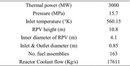
2. Geometry and Technical Data of VVER-1000 The VVER-1000 is a four loop pressurized water reactor with hexagonal fuel assembly design and horizontal steam generators. The ANSYS ICEM was used to generate the geometrical details; most of these are modelled accurately, like: inlet nozzles, outlet nozzles, downcomer, perforated elliptical sieve plate. The general characteristic of the reactor is given in Table 2.

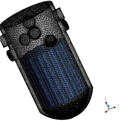
In these nuclear reactors the coolant enters the vessel by the inlets, flows downwards through the downcomer and enters the lower plenum by passing a perforated elliptical bottom plate. Then the flow crossing the core bottom plate and enters the core. The flow is heated up by the core exits from outlets. In this paper we assume that the PWR consists of vessel and 64 fuel rod assemblies. The basic geometry of considered reactor is given in Figure 1.

In this paper we only model the shell side of the reactor. From plant data the temperature profile along the fuel rod has been obtained and used in this model.

3. Calculations

3.1. The CFX-5.7.1 CODE

As noted, CFX-5.7.1 is a CFD-code using an

Table 1. Physical properties of water

ρ (kg.m-3_{) 720}

μ (kg.m-1_.s-1_{) 25.56×10}6

cp (J.kg-1.K-1) 9.0678

λ (W.m-1_.K-1₎

0.004

Table 2. The general data of VVER-1000

Thermal power (MW) 3000

Pressure (MPa) 15.7

Inlet temperature (°K) 560.15

RPV height (m) 10.8

Inner diameter of RPV (m) 4.1

Inlet & Outlet diameter (m) 0.85

No. fuel assemblies 163

element-based finite-volume numerical method with second-order discretisation schemes in space and time. It works with unstructured hybrid grids consisting of tetrahedral, hexahedral, prism and pyramid elements. The other CFX-5 options are: 1) Solution of the Navier-Stokes-Equations for steady and transient flows for compressible and incompressible fluids, 2) Modelling of heat transfers and 3) Use of different coordinate systems.

3.2. Input Deck

3.2.1. General Assumption

The following assumptions for the modelling of the coolant flow in pressurized water reactor are made: 1) incompressible fluid 2) use of the Standard k-ε turbulence model and 3) pressure boundary condition at the outlet.

3.2.2. Geometrical Simplifications, Local Details

The geometric details of the construction internals have a strong influence on the flow field and on the mixing. Therefore, an exact representation of the inlet region, the downcomer below the inlet region, the eight spacer elements in the downcomer and the lower plenum structures are necessary [13].

3.3.3. Grid Model

In order to receive an optimal net griding for the later flow simulation one must consider the following items: Checking grid number in special regions to minimize numerical diffusion, refinement of the griding in fields with strong changes of the dependent variables, adaptation of the griding to estimated flow lines, generation of nets as orthogonal as possible. In this work, the mesh contained _{1.115 10´} 6 _tetrahedral

elements and_{1.118 10´} 6 _nodes.

3.3.4. Boundary Conditions

At VVER-1000 nuclear reactor type the inlet boundary conditions (mass flow rate and temperature) were set at the inlet nozzles. No specific velocity profile was given. The wall was modelled using adiabatic conditions [14].

There were three boundary conditions imposed on the model including inlet, outlet and at the fuel rod wall.

Initial conditions fort ³0: At inlets:

0 0

z z

T ₌ =T (28)

0

r r= for all z (29)

At outlets:

0 o

z z

p ₌ =p for all z (30)

At fuel rods:

0 FR

T =T . (31)

By specifying the fuel rod’s heat transfer coefficient obtained from experiment, the fuel rod’s temperature can be calculated in CFX-5.7.1 using

(

FR

)

o FR

q h

T T

=

- , (32)

whereqFR is the heat transfer obtained from solving the

heat balance, T is the fluid temperature near the tube rods andT_FR is the fuel rod’s temperature. In this paper, we assumed that the heat flux distribution along the fuel rod is constant.

Results

Prior to the transient calculations, the steady-state was simulated. The parallel transient calculation with 10 iteration per time step took 7 hours of computation time using two processor (dual CPU computer nodes, containing 2 GB RAM). The convergence criteria were set to 1.0E-04 for RMS residuals (mass, momentum and temperature). In the calculated cases the time step of 1s was taken into account.

Figure 1. Three-dimensional image of the reactor pressure

1. Steady State Simulation

1.1. Velocity Distribution

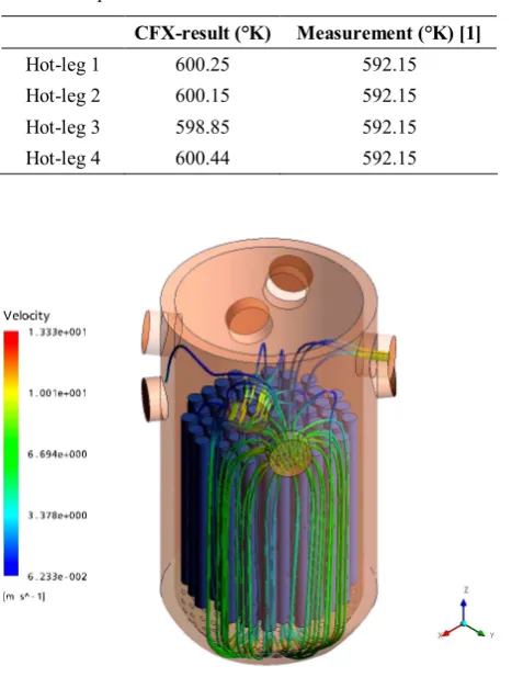
A snapshot of the velocity distribution from loop 3 in the vessel is shown in Figure 2. It is clearly seen that the flow from the corresponding loop covers a sharp sector of the vessel. The streamlines originating in this loop substantiate this finding. Mixing with the flow from the other loops takes place at the outer boundaries of the sector. There is a small layer only, where the velocity is less than 1 m/s.

1.2. Outlet Temperature Distribution

A comparison of the predicted temperature at the Hot-legs (outlet nozzles) with the plant data is showed in Table 3.

The temperature differences in the outlet nozzles are only in the range up to 2.70 °K which is not very significant. On the other hand, the temperature rise at the outlet nozzles is over-predicted by CFX-5. This discrepancy could be due to several reasons including simplification of the geometry, the grid used for the numerical simulations and/or inaccuracy in the computational model due to fluid leakage flows not being taken into account. In particular, the geometric details of the construction internals have a strong influence on the flow field and on the mixing. Herein, the flow field was computed on a three-dimensional structured grid; however, the lower plenum structures and also spacers were not included in the model, therefore, their effects on the fluid flow were not observed.

1.3. Flow Field at the Downcomer

We calculated the velocity distribution at the downcomer by CFX and this result can be seen at the Figure 3. It can be seen that the flow fields in the downcomer is not very homogenous and also no recirculation vortices are found. However, a maximum velocity exists on azimuthal positions approximately below the inlet nozzles.

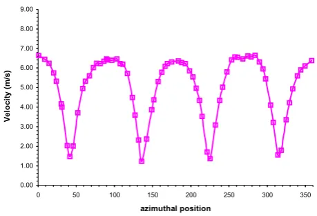
In Figure 4, the velocity at azimuthal position at the end of the downcomer is shown. As can be seen maximum velocities exist at the positions below the inlet nozzles at the end of the downcomer. There are positions between the inlet nozzles at the end of the downcomer that the fluid flow has minimum velocity.

2. Transient Simulation

Examining the streamlines presented in Figures 5 to 8 depict streamlines of water flowing in the downcomer and lower plenum of the PWR. There are four plots in

Figure 2. Snapshot of the velocity distribution in loop 3 and

the streamlines at the steady state.

Figure 3. Flow field in the downcomer at nominal conditions

(steady state).

0.00 1.00 2.00 3.00 4.00 5.00 6.00 7.00 8.00 9.00

0 50 100 150 200 250 300 350

azimuthal position

Vel

o

ci

ty (

m/

s)

Figure 4. Velocity distribution at the end of downcomer of

Table 3. Comparison of the temperature at the hot-legs in CFX and experiment

CFX-result (°K) Measurement (°K) [1]

Hot-leg 1 600.25 592.15

Hot-leg 2 600.15 592.15

Hot-leg 3 598.85 592.15

Hot-leg 4 600.44 592.15

Figure 5. Snapshots of the velocity streamlines in the

downcomer estimated by ANSYS-CFX code, 1s after start-up.

Figure 7. Snapshots of the velocity streamlines in the

downcomer estimated by ANSYS-CFX code, 40s after start-up.

Figure 4 describing the flow state at 1, 10, 40 and 80 s. At 1 s, the flow is evenly distributed around the downcomer. However, while the pump is operational and the flow rate is at 100%, the streamlines flow around the circumference of the reactor to recombine opposite the inlet position at a similar height before moving down through the diffuser and into the downcomer. Note that streamlines that move directly

Figure 6. Snapshots of the velocity streamlines in the

downcomer estimated by ANSYS-CFX code, 10s after start-up.

Figure 8. Snapshots of the velocity streamlines in the

into the downcomer after entering through the inlet loop also move around the circumference of the reactor and that there is virtually no flow down the downcomer in the region below inlet. Figures 5 to 8 depicts the streamlines in the region of the lower plenum, where the flow is passing through and around the perforated drum in order to reduce the effect of sector formation on the reactor core.

Discussion

In this paper a detailed CFD model for a whole reactor pressure vessel of a PWR-reactor of VVER-1000 type for the simulation of a coolant mixing is presented. The huge computer memory requirements of such a detailed model forced us to find a compromise between the degree of spatial resolution of some design details of the reactor components and our computational limitation. Therefore some elements in the reactor such as fuel rod assemblies are modeled in a simplified way. Nevertheless the final complete modular RPV-model consists of approximately 2 million cells. The model has been validated by the outlet temperature obtained from experiment. The mathematical background of fluid dynamics and also the CFX simulation result were discussed.

Future work is directed to the development of a model for VVER-1000 type reactors to improve the geometry and to study in more details the transient mixing behavior.

Acknowledgement

The authors like to thank Guilan’s Fanavary Park and also research deputy of the faculty of science of the University of Guilan for the support with computer facilities.

Nomenclature

p

C Specific heat (J.kg-1_.K-1₎

1 1.44

Ce = Model constant

2 1.92

C_e = Model constant

Cm = 0.09 k -ε turbulent model constant D/Dt =d/dt + v.d/dx Total derivative E Total energy per unit mass (J/kg)

e Internal energy per unit mass of a material particle (m2_.s−2₎

g Gravitational acceleration (m.s−2₎

I Unit tensor

k Turbulent kinetic energy (m2_.s−2_Kg−1₎

P Shear production due to turbulence (incompressible flows) (Kg.m-1_.s-3₎

P Static pressure (Kg.m-1_.s-2₎ '

p Modified pressure (Kg.m-1_.s-2₎

q Heat added to each material particle is at a rate per unit of Mass

qe Sources fore

k

q Sources fork

E

S Energy sources or sinks (Kg.m-1_.s-3₎ M

S Momentum sources or sinks (Kg.m-2_.s-2₎

T Temperature ( ºK ) t Time (s)

v Velocity (m.s−1₎

z Axial (m)

Greek Symbols

r Fluid mass density (kg.m-3₎

e Rate of dissipation (m2_.s-3₎

m Dynamic molecular viscosity (kg.m-1_.s-1₎ 2

t

k Cm

m r

e

= Turbulent viscosity (Kg.m-1_.s-1₎

eff t

m = +m m Effective viscosity (Kg.m-1_.s-1₎

Prt Turbulent Prandtl number (Dimensionless)

G Diffusivity (Kg.m-1_.s-1₎

Pr

t t

t

m

G = Turbulent diffusivity (Kg.m-1_.s-1₎

eff t

G = G + G Effective diffusivity (Kg.m-1_.s-1₎

k eff

eff k

m s

G = Effective diffusivity for

k

(Kg.m-1_.s-1₎

eff eff e

e

m s

G = Effective diffusivity fore (Kg.m-1_.s-1₎

1

k

s = Model constant 1.3

e

s = Model constant

l Thermal conductivity (W.m-1_.K-1₎ eff

l Effective thermal conductivity (W.m-1_K-1₎

Pr

t

eff p

t

c

m

l = +l Effective thermal conductivity (Kg.m.s-3_.K-1₎

2 3

z = m Bulk viscosity (Kg.m-1_.s-1₎

References

with the Coupled System Code RELAP5/PARCS. Progress in Nuclear Energy,48: 865-879 (2006). 2. Rohde U., Hohne T., Kliem S., Hemstromb B., Scheuerer

M., and Toppila T. Fluid Mixing and Flow Distribution in a Primary Circuit of a Nuclear Pressurized Water

Reactor-Validation of CFD Codes.Nuclear Engineering

and Design, March (2007).

3. Cartland Glover G.M., Hohne T., Kliem S., Rohde U., Weiss F.P., and Prasser H.M. Hydrodynamic Phenomena in the Downcomer during Flow Rate Transients in the

Primary Circuit of a PWR. Nuclear Engineering and

Design,237: 732-748 (2007).

4. Bieder U., Gauthier F., Sylvie B., Nikola K., and Dimitar P. Simulation of Mixing Effects in a VVER-1000 Reactor. Nuclear Engineering and Design, Feb (2007).

5. Scheuerera M., Heitscha M., Menterb F., Egorovb Y.,

Tothc I., Bestiond D., and Pignyd S. Evaluation of Computational Fluid Dynamic Methods for Reactor

Safety Analysis (ECORA). Nuclear Engineering and

Design,235: 359-368 (2005).

6. Bieder U., and Graffard E. Qualification of the CFD Code TORIO-U for Full Scale Nuclear Reactor Applications.

Nuclear Engineering and Design, In press, 2007 . 7. Bottcher M. Detailed CFX-5 Study of the Coolant Mixing

Within the Reactor Pressure Vessel of a VVER-1000 Reactor During a non Symmetrical Heat-up Test,

Benchmarking of CFD Codes for Application to Nuclear Reactor Safety (CFD4NRS), Workshop Proceedings Garching (Munich), Germany 5-7 September (2006).

8. Fox R.W., and McDonald A.T. Introduction to Fluid

Mechanics. John Wiley & Sons Inc. (1978).

9. Muralidhar K., Sundararajan T. Computational Fluid

Flow and Heat Transfer, IIT Kanpur Series of Advanced Texts. New Delhi, Narosa Publishing House (1995). 10. Ferziger J.H., and Peric M.Computational Methods for

Fluid Dynamics. Springer- Verlag (1996).

11. Wilcox D.C. Turbulence Modelling for CFD. Wilcox

Publications, La Canada, California, DCW Industries (1993).

12. ANSYS CFX, Release 10.0, Reference Guide (2005). 13. Kliem S., Kozmenkov Y, Hohne T., and Rohde U.

Analyses of the V1000CT-1 Benchmark with the DYN3D/ATHLET and DYN3D/RELAP Coupled Code Systems Including a Coolant Mixing Model Validated

Against CFD Calculations. Progress in Nuclear Energy,

48: 830-848 (2006).