*Corresponding author:Ashish Gupta ISSN: 0976-3031
Research Article
PERFORMANCE EVALUATION OF LOAD FREQUENCY CONTROL WITH
DIFFERENT TECHNIQUES WITH PID CONTROLLER
Ashish Gupta, A. D. Gupta, Yashi Gupta and R. K. Mehta
Mahamaya College of Agriculture Engineering and Technolgy
DOI: http://dx.doi.org/10.24327/ijrsr.2019.1003.3267
ARTICLE INFO ABSTRACT
Load frequency control (LFC) play a vital role in order to maintain the frequency regulation in power system. This study shows a comparative analysis of PID controller tuning methods for load frequency control in power system. Six tuning methods namely Ziegler-Nichols Method (Z-N), Tyreus-Luyben Method, Internal Model Control (IMC), Direct Synthesis Method (DS), Robust PID Controller and Optimum PID tuning for set point changes and Disturbance Rejection is adapted to evaluate their performance and used to solve the problem of load frequency control. In this paper higher order single input and single output (SISO) system is carried out with the help of Routh Approximation Method ( - expansion) and Pade Approximation Method to reduce second order model model. The performance analysis is compared to time response specification such as maximum peak overshoot, settling time, rise time and peak time and it is observed that Inter Model Control based PID Controller with first order filter exhibit better performance comparatively.
INTRODUCTION
The Power system has a long history of the trouble with the Automatic Generation Control (AGC) or Load Frequency Control (LFC) and is one of the sincerely fundamental two of researches with methodical exploration and perusal of objects and sources in order to install facts and approach new inferences of interconnected power systems. As an auxiliary service in a power system, load frequency control plays an important and fundamental role in maintaining the reliability of the power system at a reasonable level. It has been gained importance with the change in the structured of the electrical power system and growth of size and complexity of interconnected systems [1-5]. For comprehensively electrical power system, the unified and interrelated control areas are composed to load frequency. It is crucial to hold the frequency and distinction surface tie power with calculated significance power. Input mechanical power has been employed to control the frequency of the generator, variation and transformation in frequency and tie-line power, which is a measure to shift and variation in the rotor angle. A well-prepared power system should be able to provide an acceptable level of power to maintain the magnitude of the frequency and voltage within satisfactory boundaries. Some changes in the electrical power system, load especially affected the system frequency, while
the reactive power is shorted susceptive to change in the frequency and is mainly subordinate on the motility of the voltage magnitude. Therefore, the control of active and reactive power in the electrical power system is trade separately. So weight frequency control is mainly related to system frequency and actual power control, while the automatic voltage regulator loop controls is used to change in the reactive power and voltage appearance and magnitude. Load Frequency control is an elevated level of many promotions and advanced concepts, which governs the dimensions of the electrical power system. Load Frequency Control (LFC) has a basic control structure or arrangement, of parts of the machine and similar devices in term of power system operation and control. Load Frequency Control use to keep the uniform frequency during changing load. When system frequency is changed, the main problem is that the system output of generating units cannot be controlled with in specified limit is called load frequency control (LFC) [6-8]. The speed depends on the frequency of the alternative current power supply. These are the main situation when speed permanence is required to be higher order. Electrical chronometers are operated by synchronous motors. The precision of the chronometer do not depend only on the frequency but the integral part of the frequency error. If the normal frequency of any network is 50 hertz, and the network frequency falls below 48.5 hertz, and goes to high level 51.5
International Journal of
Recent Scientific
Research
International Journal of Recent Scientific Research
Vol. 10, Issue, 03(E), pp. 31472-31481, March, 2019
Copyright © Ashish Gupta et al, 2019, this is an open-access article distributed under the terms of the Creative Commons Attribution License, which permits unrestricted use, distribution and reproduction in any medium, provided the original work is properly cited.
DOI: 10.24327/IJRSR CODEN: IJRSFP (USA)
Article History:
Received 15th December, 2018 Received in revised form 7th January, 2019
Accepted 13th February, 2019 Published online 28th March, 2019
Key Words:
hertz so in this condition the blades of the turbine are damaged and all equipments of the power system like generators, governors will be damaged. When there are different loads are connected to the system in the power system then the frequency and speed will be changed due to changing the loads. If there is no need to sustain the constant frequency in a system then the manipulator does not need to change the setting of the generator. But if constant and continuous frequency expected then the manipulator can coordinate the governor characteristics and manipulated the speed of the turbine and when necessary. If variation in the load carried out, it is very difficult to run by two generating station at parallel and system is complicated and complexity becomes increases. It is very difficult to control the whole part of the power system and active power can be reflected, so the power system’s equipments may be harmful [9]. The first step to the giving gadget is that it analyzed the mathematical modeling of the system’s variety of factors and make use of the control system technology. There are different modes of electrical drives loaded on the electricity system. The instruments used for irradiation purposes are basically resistive in nature and rotating devices are basically combinatorial with resistive and inductive components. The electrical power is greater from mechanical power input, the electric load increased. As a result, the power shortage in the load side is derived from the rotating energy of the turbine. This is a suitable motive for the kinetic power of the turbine i.e. the stored energy is decreased in the machine and the governor dispatch a signal to supply the excess quantity of water or vapor or gas to speed up the prime mover to restitute for the shortage of speed. Visioli in this paper, suggested that even after so much advancements in control theory there is a lot of scope for research in PID controllers, since it is renowned that generally controllers are not tuned properly in industrial applications, and the performance that is recognized can be enhanced several times by using a more accomplished construction prescript for the PID-based control system. In this paper we described many important results achieved recently in the field of PID controllers, and reviews in particular those related to tuning and designing PID-based control fabrication [10]. The control system performs poor and even it will be unstable, if the values of PID parameters adjust improper. So it is necessary to tune the parameter of PID controller in the appropriate option by which good control performance may be obtained. There are many tuning methods which are used to tune a PID controller.
LFC Design without Droop Characteristics
There are three different types of turbines consisted in without droop characteristics.
Governor with Dynamics
s
s
G
a a
1
1
)
(
1Turbine with Dynamics
s
s
G
c c
1
1
)
(
2Load and Machine with dynamics:
s
K
s
G
l l l
1
)
(
34) 1/R is the droop characteristics a kind of feedback gain to improve the damping properties of the power system
Non-Reheated Turbine [11]
The open loop transfer function without droop characteristic of load frequency control (LFC) is:
)
(
)
(
)
(
)
(
s
G
s
G
s
G
s
P
a c l 4
)
1
)(
1
)(
1
(
)
(
s
s
s
K
s
P
l c
a l
5The open loop transfer function of load frequency control (LFC) is [12]
)
(
)
(
)
(
)
(
s
G
s
G
s
G
s
P
a c l 6)
1
)(
1
)(
1
(
)
(
s
s
s
K
s
P
l c
a l
7l
K
=120,
c=20,
b=0.3,
a=0.08, R=2.4)
20
1
)(
3
.
0
1
)(
08
.
0
1
(
120
)
(
s
s
s
s
P
83 2
120
( )
0.48
7.624
20.38
1
P s
s
s
s
9
Governor Turbine Load & Machine Droop
Characteristics
_ Pg
Pt Pl Fo
Pd
U
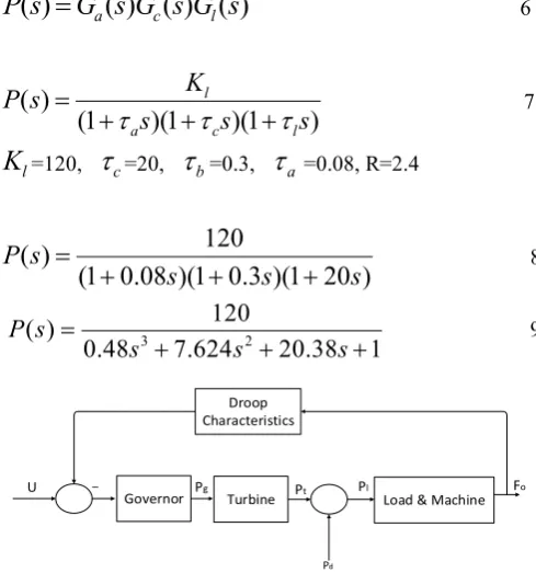
Fig 1 A single area Power system with droop characteristics
The feedback gain is used in power system is known as droop characteristics and it is used to improve the damping properties of power system and it is generally represented as 1/R and connected before load frequency control design. So there are two ways for LFC design.
The open loop transfer function with droop characteristic of load frequency control (LFC) is:
( )
1
/
g t p
g t p
G G G
P s
G G G
R
3 2
( )
( ) ( ) (1 / )
p
p t g p t t g p g p t g p
K P s
T T T s T T T T T T s T T T s K R
11
3 2
120
( )
0.48
7.624
20.38
51
P s
s
s
s
12MOR Techniques- [12-15]
The nth higher order model for the continuous system which is not feasible because of its unsatisfactory performance. Now we are trying to find a rth reduce order system or process for the original model having desired performance, where r is a random number and r<n. Also the reduced model should be fairly accurate to the original process so the results starting the state space of reduce model and the original model should also be approximate. The main motive of this process is to find a simplified model with reduced complexity and cost with the desired performance. In this section, the higher order transfer function of the LFC system has been Figure 2 it can seen the PID controller with component transfer function of LFC system. With these components transfer function calculation of the closed loop response of LFC system has been done. The reduced order model for the LFC system with applied six different techniques can be listed below:-
_
+ Pg Pt Pl
Pd
1/R
i
p d
K K Ks
s
1
1
ts
1 1
gs
1
l
K s
PID Controller Turbine Governor Load
Figure 2 A practical high-order LFC system controlled by a PID controller
94
.
7
173
.
3
68
.
18
)
(
2
s
s
s
G
RouthMR
13
043
.
8
708
.
2
92
.
18
91
.
1
)
(
2
s
s
s
s
G
PadeMR 14
It has been observed that the parameters of controllers vary for different tuning method. Futher in next chapter we concluded the result analysis and conclusion. The results show all the details about design analysis for different six tuning method with and without controller.
Generalised Model of PID Controller
PID controllers are the majorly used controllers in industries because of their robustness and the overall performance of super management. Apart from this, PID controllers are trouble-free and easy to execute. The PID controller contains the three basic components; namely Proportional control, Integral control and Derivative control. All these components of PID controller have certain specific effects on the process. The tuning parameters which are determined to tune the PID controller are the respective gain values of PID such as: Proportional gain
(
K
P)
, Integral term(
K
i)
and Derivativegain
(
K
D)
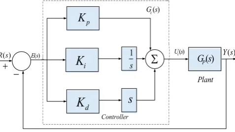
. These benefits affect the procedure in a sure way. It means that these parameters have the tendency to change the characteristics of the process. Since the LFC system to maintain the fluctuating frequency to a constant value, it isrequired to understand the reason of variability in the frequency of the alternator at its terminus. The main reason of the variation in the frequency is the load variations which are acting upon the supply system. These variations in the load and hence in the voltage, may lead to functioning of the power system, due to damage of various equipments of power system. Hence, it is highly required to control the voltage and loads of a turbine and governor. This work describes the various methodologies and technique to control the terminal voltage of the system through LFC system. The terminal voltage and frequency can be controlled through various control techniques. However, PID control technique is the most commonly utilized controllers in industries. The next section discusses a basic and concise principle about the PID controller. The figure 3 demonstrated a basic structure of the PID controller.
p
K
i
K
d
K
1
s
s
G sP( )( )
R s
( )
E s Y s( )
Plant
( )
c
U s
( )
c G s
Controller
Fig 3 Structure of PID controller
For the desired response from the given plant, the PID controllers need to be tuned effectively. The behavior of the plants depend the tuning parameters of the PID controller. The PID controller shall be tuned in such a way that it can withstand the various disturbances and keep the response of the plant with in desirable limits. Tuning of the controller simply means the selection of three gains viz: Proportional gain (Kp), Integral gain (Ki) and derivative gain (Kd). These gains can be obtained through various tuning techniques developed for PID controller. The output of the PID controller actually depends upon these three types of gains and is depicted in equation 19. In spite of, the Integral and Derivative gains rely upon the Integral time constant (Ti) and Derivative time constant (Td) respectively. Gp(s) represents the LFC system transfer function and Tf(s) indicates the sensor transfer system and Gc(s) is the controller transfer function. Hence, the controller’s output in term of the time constant is given in equation 115. The PID controller may be written in the following manner. [16-20].
)
(
1
1
(
)
(
)
(
)
(
T
s
s
T
K
s
E
s
U
s
G
di p c
c
15( )
pc p p d
i
K
G S
K
K T s
T s
16( )
ic p d
K
G s
K
K s
s
17 PID controller can be systematized in the form of close-loopin the form of parallel and series form. The PID controller has many types of different structure-
Idealstructure
1
1
( )
1
c c d
i
G
s
K
s
s
18 SeriesStructure
2
1
1
( )
1
1
d
c c
i d
s
G
s
K
s
s
19
ParallelStructure
3
1
( )
1
1
d
c c
i d
s
G
s
K
s
s
20
Seriesfilter
4
1
1
( )
1
1
c c d
i f
G
s
K
s
s
s
21 Where,
Uc(s) - Control signal, E(s) - Error signal,
R(s) – Reference signal, and Y(s) – Output of LFC
In PID designing, the parameters of controller must be tuned in this way that the closed loop system meets for Robustness in stability, it often precise in domain of frequency, Transitory response includes rise time, settling time and overshoot and Accuracy in immovable situation distinction.
Governor Turbine Load & Machine
_
+ Pg Pt Pl
Pd
PID Controller
1/R
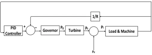
Fig 4 Block diagram of PID controller with LFC
Design PID Controller Techniques
Ziegler-Nichols Method (Z-N)
(Ziegler, and Nichols 1942) [21] is a vastly utilitarian tuning technology to design PID controller. ZN method is of two types- one is based on reaction curve of the system and other one depends upon ultimate gain Ku and ultimate period Tu when step response of the plant exhibits s-shape curve with zero overshoot than reaction curve method is applied. The traction curve is described through two consecutive parameters, which delay time L and time constant T. Second method considers trial and error tuning which based on proportional gain Kp by increasing the value of Kp output exhibit sustains oscillations. This rule works well only when delay time is less than half the length of time constant. The disadvantage of this technique is that it is time consuming and this is not applicable for first and second without time delay process because some process does not have ultimate gain. The method performs well in disturbance rejection but poor in tracking reference change.
Table 1 Controller Settings for ZN
Type of Controller
Parameter of Controller
P
K
T
IT
DP
0.5
U
K
--PI
0.45
K
U0.84
T
U -PID
0.6
K
U0.5
T
U0.125
T
UTyreus-Luyben Method
The Tyreus-Luyben Method [22] is a same process to the Ziegler-Nichols method but the final value of controller setting is different than Ziegler-Nichols technique. This method use only PI and PID conytrollers. It depends upon ultimate gain Ku and ultimate period Tu when step response of the plant exhibits s-shape curve with zero overshoot than reaction curve method is applied.
Table 2 Controller Settings for TL
Type of Controller
Parameter of Controller
P
K
T
IT
DPI
0.45
U
K
2.2
T
UPID
0.45
U
K
2.2
T
U6.3
U
T
Internal Model Control (IMC)
There are many method of tuning IMC-PID based controller [23-24] but first method was developed by Morari et. al. (1986) for tuning parameter which is called Internal Model Control. This method is based on model based control technique. Internal Model Control (IMC) based PID controller [25] is encompassed in manufacturing, technical and insdustrial control structure. The design gives a superior concession along with set point tracking, disturbance rejection and robustness. In fact, in the Internal Model Control, the original model of the system agglutinated in parallel form with the help of model of the plant and fed back to the controller is shown as the distinction between the process and the process model. The advantage of this approach is good set point tracking, but sluggish trouble response, especially when there is a continuous ratio of time / time in the process. This process is not desirable for the industry because the application point for many control procedures is more important than troubleshooting rejection sets point tracking Li et al. (2000). The general block diagram IMC based approach shown in figure 5. This diagram is used to control the process in Ac(s), Ap(s) process, model Am(s) and D (s) is unknown turbulence. Now, instead of taking model precisely same as plant, we consider the reduce order model of the original system, i.e., P(s)= PMOR to acquire controller. To demonstrate this process, let the original system be
1 2
1 2 0
1 2
1 2 0
...
( )
,
...
m m m
m m m
n n n
n n n
a s
a
s
a
s
a
P s
m n
b s
b s
b s
b
Controller Ac(s)
Process Ap(s)
Process Model Am(s) U(s)
D(s)
R(s) ++
+ _
C(s) +
_
Fig 5 Basic Block diagram of Internal Model Control.
Using MOR, the reduced model can be written as 1
( )
(
1)
MOR
P
s
K s
23Where K and
are constants. The above PMOR(s) can be determined by various MOR techniques as reported in control literature. The next step is to include this model for IMC-PID design. In case, if the plant is of first order type then PI is requisite for IMC technique. For second order type system it is found that IMC-PID is required in consideration of IMC procedure. Furthermore, the most interesting feature is that all the parameters of controller (Kp, Ki, Kd) depend on a value of single user-defined parameter
in case of IMC based PID control. The generalized form of controller is given by as follow:-1
( )
p i dC s
K
K s
K s
24 We adopt a two degree of freedom IMC-PID tuning method forload frequency controller. The method for SOPDT model goes as follows.
Design an IMC controller
2 2
2 2
2
( )
(
1)
n n
n
s
s
Q s
k
s
25Here
is a tuning parameter such that the desired setpoint response is1
2(
s
1)
.(2) Design a controller of the form 2
2
1
( )
(
1)
d
d
s
s
Q s
s
26Where
dis another tuning parameter for disturbance rejection.
2 4 1 4
1 2 2 1 1 2
1 2 2 1
( 1) ( 1)
( )
p p
f f
p e p p e p p p
p p p p
27
2 1
2 4 2 4 2 2
1 2 2 1 1 2
1 2 2 1
( 1) ( 1)
( )
p p
p e p p e p p p
p p p p
28
Transform it to a Conventional Unity Feedback Controller
( )
( )
( )
1
( ) ( )
( )
d
d
Q s Q s
K s
P s Q s Q s
29
Direct Synthesis Method (DS)
Direct Synthesis approach [26-27] has consisted on the way of PID controller and the desired closed loop transfer function is introduced for the describing and identifying of system’s disturbances. Analytical expression process model for PID controllers is taken for many common types, along with first order, including dead time, second order along with dead time model. The Direct Synthesis method is similar to internal model control technique. Fig 6 show basic closed loop system structure of the process. Where Gp is the process, it is controlled by the controller (Gc) and Gv is the actuator and Gc is the Direct Synthesis (DS) controller to design.
K Gc
Gd
Gp Gv
Gf
Yi Ya
+ _
E P U Yu Y
Yd
D
Ym
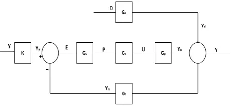
Fig 6 Basic Block diagram of Direct Synthesis (DS).
Design an DS Controller
For easy implementation of PID controller, Gc is considered in the following form.
1
1
1
d
c c
i d
T s
G
K
T s
T s
30 Where the derivative filter constant is typically fixed by the manufacturer and
=0.1. The nominal complementary sensitivity for load disturbances rejection can be obtained as1
cc
GG
T
GG
31In order to reject a step change in load of power system, the asymptotic constraint should be satisfied so that the close loop internal stability can be achieved. The desired closed loop complementary sensitivity function is as-
2
2 1
4
(
1)
(
1)
ms
s
s
T
e
s
32
2 4 1 4
1 2 2 1 1 2
2
1 2 2 1
( 1) ( 1)
( )
p p
p e p p e p p p
p p p p
33
2 1
2 4 2 4 2 2
1 2 2 1 1 2
1
1 2 2 1
( 1) ( 1)
( )
p p
p e p p e p p p
p p p p
34
Where p1 and p2 are the two poles of the reduced model Where P1 and P2 are the two poles of the process. When
1
, there exists P1=P2=
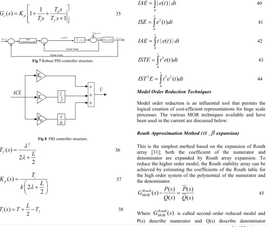
n.Robust PID Controller
Robust controller [28] deal with plant uncertainty. If there is slight change in gain K, time constant T and delay time L Robust controller will provide uncertainty and achieves robustness and stability here we are calculating PID parameter for FOPDT system which based on
H
control theory. The performance of PID is determined by value of
. Here we choose value of tunable parameter
is 0.1 respectively and 0.3 respectively.
1
( )
1
1
dc p
i f
T s
G s
K
T s
T s
35
PID CONTROLLER
Inner loop
Outer loop
) (
2 s
G G1(s)
) (s R
) (
1s d
) (
2s
u u1(s) Y(s)
Fig 7 Robust PID controller structure.
dt d
P
K
I
K
D
K
U
ACE
Fig 8 PID controller structure.
2
( )
2
2
fT s
L
36
( )
2
2
i pT
K s
L
k
37
( )
2
i f
L
T s
T
T
382
d f
i
TL
T
T
T
39Optimum PID Tuning for set Point Changes and Disturbance Rejection [29-30]
The shape of close loop response of the system from initial state t=0 to final state could be used to find exact controller setting. To reduce the use of these rules, the PID controller is used to get the optimum tuning value of the parameter Integral Square Error (ISE), Integral Absolute Error (IAE), Integral time Absolute Error (ITAE), Integral Square Time Error (ISTE), Integral Square Time Square Error (IST2E) performance criteria. These tuning formulas were found by (zhuang and Atherton 1993), IAE is good to eliminate small error but it produces slower response and it does not add weight for any error in response. To use this harmful ITAE and ITE performance criteria, ISE will bear short errors, short dimensions, small errors for the charge for long periods, which settles faster than other two because it integrates the absolute value of error multiplied by time (Rahimi & Famouri 2014).
0
| ( ) |
t
IAE
e t
dt
402
0
( )
t
ISE
e t dt
410
| ( ) |
t
IAE
t e t
dt
422
0
( )
t
ISTE
t e t dt
432 2 2
0
( )
t
IST E
t e t dt
44Model Order Reduction Techniques
Model order reduction is an influential tool that permits the logical creation of cost-efficient representations for huge scale processes. The various MOR techniques available and have been used in the current are discussed below:
Routh Approximation Method (
-
expansion)This is the simplest method based on the expansion of Routh array [31]; both the coefficient of the numerator and denominator are expanded by Routh array expansion. To reduce the higher order model, the Routh stability array can be achieved by estimating the coefficients of the Routh table for the high order system of the polynomial of the numerator and the denominator.
)
(
s
G
MORRouth =)
(
)
(
)
(
)
(
s
Q
s
P
s
Q
s
P
45respectively. We first interchange
G
MORRouth(
s
)
using rapport
s
L
s
s
L
(
)
1
1
. Thus the reciprocated model of G(s) occurs-A
Bs
Cs
Ds
Ks
s
G
3 22
)
(
46And then, enhance
G
(
s
)
, namely
t j j n t t ii
F
s
s
Q
s
P
s
G
1 1)
(
)
(
)
(
)
(
47Where
i(
i
1
,
2
)
are constant and Fi(s) (i=1,2) contains
iterms. Next, we need to compute
and
tables corresponding to, which is shown in table 1.7.are reported in [26]. These
and
terms gives reciprocated reduce-order numerator P(s) and denominator Q(s) for second order reduced model as-
s
s
P
(
)
b
b
a 482
1
)
(
s
s
s
Q
b
a
b 49 On substituting values of
and
in (1.38) and (1.39), we get
BC
AD
CKs
s
P
)
(
50
BC
AD
CDs
AD
BC
s
C
s
Q
2 21
)
(
51
BC
AD
s
C
s
CD
CK
s
G
MORRouth
2 2)
(
52Table 3
-
table for Routh approximation
Table
TableC
D
a
C
K
a
AD
BC
C
b
2
b
0
Pade Approximation Method
The coefficient of the original model is reduced by using reduction method [32] with the help of coefficient of Taylor series expansion about s=0. In order to convert higher order system G(s) into second order reduced model
G
MORPade(
s
)
, we define as- j i j i Pade MORb
s
b
s
a
s
a
s
G
2(
)
)
(
53 Let suppose system is given as;D
Cs
Bs
As
K
s
G
3 2)
(
54
A
D
s
A
C
s
A
B
s
A
K
s
G
2 3)
(
55Power series expansion can be articulated like the colligation of G(S).
...
)
(
s
C
0
C
1s
C
2s
2
C
3s
3
G
56Where,
D
K
C
0
, 1 2D
CK
C
,
3
2 2
D
K
BD
C
C
,
4 3 2 32
D
K
C
AD
BCD
C
57Now, second order reduced order model
G
MORPade(
s
)
can be obtained from mentioned in this equation, the parameter ai and bi (i=0,1) can be estimated by illuminate -= −− , = 0 58
Comparative Analysis
In this section, a comparative view of all the algorithms used to design PID controller for LFC system has been presented.
Fig 9 Step response with reduced model with droop characteristics
Table 4 Reduced Model with Non-Reheated Turbine
Sys Mp(%) Tr(sec) Ts(sec) Tp(sec) ITAE IAE ISE Plant 19.2496 0.5712 3.0161 1.3497 - - - Routh 11.7532 0.6278 2.0808 1.3353 1.38 0.4336 0.05125
Fig 10 Frequency response with reduced model with droop characteristics
Fig 11 Nyquist plot with reduced model with droop characteristics
Fig 12 Pole-Zero plot with reduced model with droop characteristics
Responses of Systems with Controller
In this section the results presented for each system (original and reduced); when the designed controllers have been applied to each system. Figure 13
Figure 13 Step response for given process with PID tuning techniques
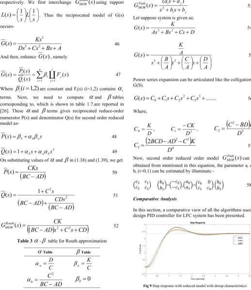
Figure 14 Bode plot for given process with PID tuning techniques
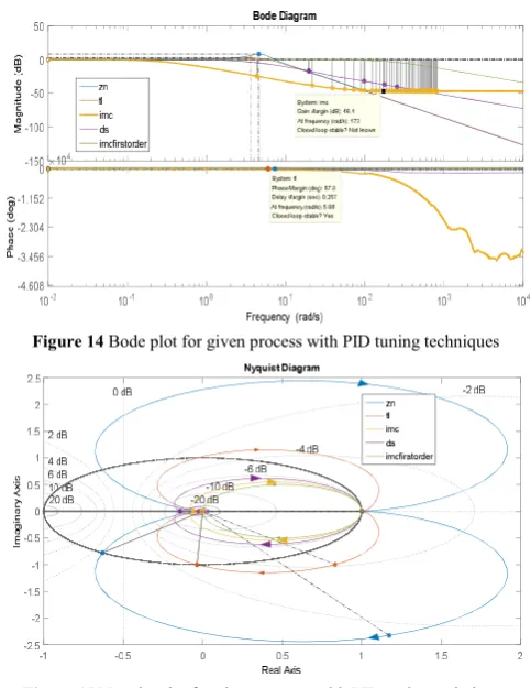
Figure 15 Nyquist plot for given process with PID tuning techniques
Table 5 Comparative Analysis of PID Tuning Techniques
Process Mp(%) Tr(sec) Ts(sec) Tp(sec)
Plant 0 43.9456 78.6278 146.4444 ZN 60.4726 0.2013 3.3803 0.5807 TL 25.6365 0.2554 2.4737 0.6251 IMC 0 8.3368 15.3738 26.7997
DS 0 0.7014 1.3325 3.2254 IMCfirstorderfilter 0 0.0110 0.0196 0.0527
Robust PID
Controller 0 1.839 3.3216 6.0372
Figure 17 Comparison between reduced order LFC with Controller
Figure 4.23 show the compare between five techniques [ZN, TL, DS, Robust PID Controller and IMC based first order filter]. IMC based first order filter give a best response than ZN, TL, DS and Robust PID controller about frequency deviation and set point.
CONCLUSION AND RESULT
The work described in this report has been carried out to test the performance of LFC system. Since the frequency is the crucial parameter and needs to be controlled precisely. For this purpose and Load Frequency Control is used in power system. The performance of LFC has been tested with the PID controller. For this work, the original LFC model has been reduced to lower order using different MOR techniques. Then the PID controller is designed for each reduced system. The PID controller has been tuned using five different techniques viz; Z-N, T-L, IMC, DS and Robust PID controller tuning methods. The performance of each reduced system has been tested for for tuning techniques. Then the performance of original system has been tested for the same PID controllers. For the analysis it has been observed that Robust PID controller with first order plus dead time (FOPDT) reduced order process and Internal Model control with filter give the better performance among all other methods. In the present work, the LFC system has been studied on reduced order by applying various model order reduction techniques and finding the reduced order transfer function of LFC. To identify the LFC and develop its Mathematical model and to develop and design PID tuning techniques for LFC and reduced order modeling of the third order transfer function of the LFC of the research have been briefly discussed. In the next Chapter, the problem formulation discussed and the the main focus will be on to design the desired optimal controller. So, to accomplish the stated problem and desired performance of the Load Frequency Control for the current work, some objectives have been identified which are listed below- To identify the LFC and develop its Mathematical model and To develop and design PID tuning techniques for LFC.
References
1. P. Kundur, “power system stability and control, ” New YorkP: McGraw Hill, 1994.
2. N.N. Bengiamin and W.C. Chan, “Variable structure control of electric power generation, ” IEEE Trans. Power App. Syst., pp. 2271-2285, 1972.
3. S. Sondhi and Y.V. Hote, “Fractional order PID Controller for load frequency control, ” Energy convers. Manag., pp. 343-353, 2014.
4. M.N. Anwar and S. Pan, “A new PID load frequency control design method in frequency domain through Direct Synthesis approach, ” Elec. Power & Energy syst., pp. 560-569, 2015.
5. A. Demiroren, N.S. Sengor, and H.L. Zeynelgil, “Automatic generation control by using ANN technique,” Electrical Power component system, pp. 883-896, 2001.
6. R.K. Cavin, M.C. Budge, and P. Rasmussen, “An optimal linear system approach to load frequency control,” IEEE Trans. Power App. Sys., pp. 2472-2482, 1971.
7. M. Calovic, “Linear regulator design for a load and frequency theory, ” IEEE Trans. Power App. Syst., pp. 2271-2285, 1972.
8. C.T. Pan and C.M. Liaw, “An Adaptive controller for power system load frequency control, ” IEEE Trans. Power syst., pp. 122-128, 1989.
9. M. Azzam, “Robust automatic generation control, ” Energy convers. Manage., pp. 1413-1421, 1999.
10. A. Khodabakhshian and N. Golbon, “Robust load frequency controller design for hydro power system, ” in proc. IEEE conf. control application (CCA), pp. 1510-1515, 2005.
11. G.A. Chown and R.C. Hartman, “Design and experience with a fuzzy logic controller for automatic generation control, ” IEEE Trans. Power Syst., pp. 965-970, 1998. 12. J. Talaq and F. Al-Basri, “Adaptive fuzzy gain
scheduling for load frequency control,” IEEE Trans. Power Syst., pp. 145-150, 1999.
13. H. Shayeghi and H.A. Shayanfar, “Application of ANN technique based on μ- synthesis of load frequency control of interconnected power system,” Electrical power energy syst., pp. 503-511, 2006.
14. S. Baghya Shree and N. Kamaraj, “Hybrid neuro fuzzy approach for automatic generation control in restructured power system,” Electrical power energy syst., pp. 274-285, 2016.
15. H. Zenk and A.S. Aspinar, “Two differewnt power control system load frequency analysis using fuzzy logic controller, ” IEEE, pp. 465-469, 2011.
16. M. Mahdavian and N. Wattanapongsakorn, “Load frrequency control for a two area HVAC/HVDC power system using hybrid genetic algorithm controller, ” IEEE, pp. 1-4, 2012.
17. S.K. Gautam and N. Goyal, “Improved partical swarm optimization based load frequency control in a single area power system, ” IEEE, pp. 1-4, 2010.
19. S. Sondhi and Y.V. Hote, “Fractional order PID controller for load frequency control,” Energy conversion and manage., pp. 343-353, 2009.
20. R.C. Panda, C.C. Yu, and H.P. Huang, “PID tuning rules for SOPDT system review and some new results, ” ISA Trans., pp. 283-295, 2004.
21. M. N. Anwar and S. Pan, “A new PID load frequency controller design method in frequency domain through direct synthesis approach” International Journal of Electrical Power and Energy Syst., pp. 560-569, 2015. 22. D. Chen and D. E. Seborg, “PI/PID controller design
based on Direct Synthesis and Disturbance Rejection”, Ind. Eng. Chem. Res., pp. 4807-4822, 2002.
23. M. shamsuzoha and S. Skogestad, “The setpoint overshoot method, A simple and fast close-loop approach for PID tuning”, Journal of Process Control, pp. 1220-1234, 2010.
24. A. Visioli, “Research Trends for PID Conreoller”, Acta Polytechnica, pp. 144-150, 2012.
25. D.K. Saini and R. Prasad, “Order Reduction of Linear Interval Systems using Particle Swarm Optimization”, MIT International Journal of Electronics and Instrumentation Engineering, pp. 16-19, 2011.
26. G. Langholz and D. Feinmesser, “Model reduction by Routh approximation”, Internationaql Journal of systems Science, pp. 493-496, 1978.
27. B. Bandyopadhyay and S. Lamba, “Time-domain pade approximation and modal-Pade method for multivariable systems”, IEEE Transactions on Circuits and Systems, pp. 91-94, 1987.
28. S. Skogestad, “Simple analytic rules for model reduction and PID controller tuning”, J. Process Control, pp. 291-309, 2003.
29. A. Sikander and R. Prasad, “Linear time invariant system reduction using a mixed methods approach”, Applied Mathematical Modelling, pp. 4848-4858, 2015 30. M. F. Hutton and B. Friedland, “Routh Approximation
for Reducing order of Linear Time-Invariant Systems”, IEEE Transactions on Automatic Control, pp. 329-337, 1975.
31. Y. Shamash, “Stable Reduced Order Models using Pade Type Approximation”,IEEE Transaction on Automatic Control, pp. 615-616, 1974.
32. V. Singhal and R. Singh, “Design and performance Analysis of tuning Conventional Controllers and Fuzzy Controllers PID approach for Automatic Voltage Regulator”, International Journal of Modern Trends in Engineering and Research, pp. 269-277, 2017.
How to cite this article:
Ashish Gupta et al., 2019, Performance Evaluation of Load Frequency Control with Different Techniques with Pid Controller. Int J Recent Sci Res. 10(03), pp.31472-31481. DOI: http://dx.doi.org/10.24327/ijrsr.2019.1003.3267