ORIGINAL ARTICLE
Closed-Form Modeling and Analysis
of an XY Flexure-Based Nano-Manipulator
Yan‑Ding Qin
1*, Xin Zhao
1, Bijan Shirinzadeh
2, Yan‑Ling Tian
3and Da‑Wei Zhang
3Abstract
Flexure‑based mechanisms are widely utilized in nano manipulations. The closed‑form statics and dynamics modeling is difficult due to the complex topologies, the inevitable compliance of levers, the Hertzian contact interface, etc. This paper presents the closed‑form modeling of an XY nano‑manipulator consisting of statically indeterminate symmet‑ ric (SIS) structures using leaf and circular flexure hinges. Theoretical analysis reveals that the lever’s compliance, the contact stiffness, and the load mass have significant influence on the static and dynamic performances of the system. Experiments are conducted to verify the effectiveness of the established models. If no piezoelectric actuator (PEA) is installed, the influence of the contact stiffness can be eliminated. Experimental results show that the estimation error on the output stiffness and first natural frequency can reach 2% and 1.7%, respectively. If PEAs are installed, the con‑ tact stiffness shows up in the models. As no effective method is currently available to measure or estimate the contact stiffness, it is impossible to precisely estimate the performance of the overall system. In this case, the established closed‑form models can be utilized to calculate the bounds of the performance. The established closed‑form models are widely applicable in the design and optimization of planar flexure‑based mechanisms.
Keywords: Flexure‑based mechanism, Statically indeterminate structure, Dynamics, Lever mechanism, Piezoelectric actuator
© The Author(s) 2018. This article is distributed under the terms of the Creative Commons Attribution 4.0 International License (http://creativecommons.org/licenses/by/4.0/), which permits unrestricted use, distribution, and reproduction in any medium, provided you give appropriate credit to the original author(s) and the source, provide a link to the Creative Commons license, and indicate if changes were made.
1 Introduction
The integrations of piezoelectric actuators (PEAs) and flexure-based mechanisms have been widely utilized in nano-positioning and manipulations [1–5]. On the one hand, the shape of a PEA changes if charge or voltage is exerted, and thus generating sub-nanometer resolu-tion actuaresolu-tion. However, PEAs suffer from the inherent hysteresis and creep nonlinearities [6–8]. Many feedfor-ward and feedback methodologies have been proposed to compensate for the hysteresis and creep nonlinearities of PEAs [9, 10]. On the other hand, flexure-based mecha-nisms are capable of transmitting high-precision motions via the elastic deformations of the flexure hinges, making it ideal in building the transmission chains for PEAs [11,
12]. Widely utilized flexure hinge profiles include circular [13–16] and leaf [17, 18].
A single flexure hinge can be treated as a revolute joint during micro- and nano-scale motions. In litera-ture, many analytical and empirical models have been established for the compliance/stiffness of a single flex-ure hinge [19–21]. In order to improve the performance, multiple flexure hinges are generally combined in various configurations, such as the parallelograms [22–24] and the statically indeterminate symmetric (SIS) structures [25]. In these structures, it is common to treat the flexure hinges as flexible, and all the other components as rigid. Considering the widely-utilized lever mechanism as an example, the lever is frequently assumed to be rigid [26,
27] so as to facilitate the design and modeling processes. However, this assumption may increase the estimation error of the analytical model, especially when the lever is long or the compliance of the lever is not negligible.
A PEA is brittle and very weak when subjected to large lateral forces or torques. As a result, a PEA is not allowed to be firmly fixed to the mechanism during the installa-tion. Many commercial PEAs use ball tips to eliminate the bending torques. In this case, a Hertzian contact
Open Access
*Correspondence: [email protected]
1 Institute of Robotics and Automatic Information System (Tianjin Key Laboratory of Intelligent Robotics), Nankai University, Tianjin 300350, China
interface forms between the tip and the mechanism. One significant drawback of Hertzian contact is its low con-tact stiffness that consumes large portion of the PEA’s displacement. The contact stiffness is highly dependent on the material properties and the contact status. Cur-rently, there is no effective and reliable model to estimate the contact stiffness. Thus, the contact stiffness is fre-quently identified from the measured data [2].
As a flexure-based mechanism is generally light and compact, its performance is likely to be affected by the load mass, including the sensors, end-effectors, fixtures, and other accessories installed on the mechanism. The load mass increases the effective mass and moment of inertia of the system, leading to a slow response. Thus, the influence of the load mass should be taken into con-sideration in the design and modeling of flexure-based mechanisms.
This paper presents the closed-form modeling of an XY flexure-based nano-manipulator developed in our previous work [28]. In this nano-manipulator, the flex-ure hinges are arranged in SIS configurations to transmit linear or angular motions. Analytical modeling reveals that the lever’s compliance significantly increases the estimation error. Thus, a threshold is proposed to deter-mine whether the lever’s compliance can be neglected or not. Subsequently, a systematic modeling method-ology is established to investigate the behavior of the nano-manipulator during linear and angular motions. Experimental results show that the modeling accuracy is significantly improved if the influence of the lever’s com-pliance, the contact stiffness, and the load mass is taken into consideration.
2 Design of the XY Nano‑manipulator
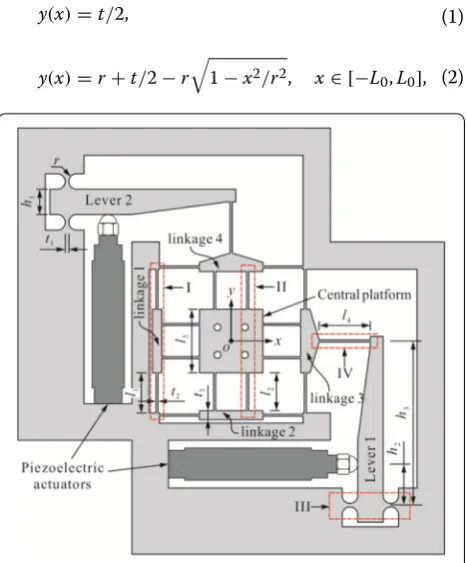
An XY flexure-based nano-manipulator was devel-oped for nano manipulation tasks in our previous work [28]. The schematic diagram and the geometric param-eters of the nano-manipulator are presented in Figure 1, where a central platform is connected to four rigid link-ages (consecutively labeled as linkage 1‒4) and then to the fixed frame through leaf springs. The nano-manip-ulator is symmetric in the x- and y-axes, thus attenuat-ing thermally induced errors and guaranteeattenuat-ing uniform characteristics. In each axis, the displacement of a PEA (P-843.30 from Physik Instrumente) is magnified by a lever mechanism. Ball tip is selected to form a Hertzian contact interface so as to protect the PEA against the lateral forces and torques. Leaf and right circular flex-ure hinges are adopted in the manipulator. These flexflex-ure hinges are arranged into four different groups, namely Structure I-IV (labeled as I-IV in Figure 1). Except for Structure IV, the other structures are SIS structures with “clamped-clamped” boundary conditions. Experimental
results showed that the cross-axis coupling ratio of the nano-manipulator is below 1% [28].
3 Characteristics of the SIS Structures 3.1 In‑plane Compliance of a Single Flexure Hinge
Leaf and right circular flexure hinges are utilized in the nano-manipulator. As illustrated in Figure 2, the geo-metric parameters are the hinge length 2L0 and the mini-mum thickness t. The shape functions of these hinges are defined in Eqs. (1) and (2), respectively:
(1)
y(x)=t/2,
(2)
y(x)=r+t/2−r
1−x2/r2, x∈ [−L0,L0],
Figure 1 Schematic diagram of the nano‑manipulator. t1, t2: Minimal
thickness of circular and leaf flexures, t1 = 0.58, t2 = 0.44, t3: Thickness
of linkages, t3 = 4, r: Radius of the circular flexure hinge, r = 3.41, t1, t2,
t3: Parameters of the lever mechanism, h1 = 11.1, h2 = 18, h3 = 72, l1,
l2, l4: Length of leaf flexures, l1 = 17.61, l2 = 16.61, l4 = 22.39, l3: Width
of the central platform, l3 = 27.78, d: Out‑of‑plane depth of the nano‑
manipulator, d = 20.
where r is the radius of the circular profile, and for the right-circular flexure hinge, r = L0.
As shown in Figure 2, the in-plane loads of the flex-ure hinge are the moment about the z-axis (Mz) and two forces in the x- and y-axes (Fx and Fy). The angular deflec-tion about the z-axis and the linear deflections in the x- and y-axes are denoted as θB, uB, and vB, respectively. The bending moment Mz(x) and shear force Q(x) generated at position x may be written as
In the x-axis, the linear deflection at point B is defined by the following equation:
where E is the Young’s modulus, A(x) = 2dy(x) is the cross sectional area of the hinge, and
Subsequently, the angular deflection of point B about the z-axis can be modeled as
where Iz(x) = 2dy3(x)/3 is the second moment of area with respect to z-axis, and
Timoshenko beam theory is utilized to calculate the linear deflection in y-axis:
where θ(x) denotes the angular deflection at position x,
G is the shear modulus, κ is the Timoshenko shear coef-ficient, and
(3)
Mz(x)=Mz+Fy(L0−x),
Qy(x)= −Fy.
(4)
uB= L0
−L0 Fx
EA(x)dx=
Fx 2Ed
L0
−L0
1
y(x)dx=FxP1,
P1=
1 2Ed
L0
−L0 1
y(x)dx.
(5) θB=
L0
−L0 Mz(x)
EIz(x)
dx= 3(Mz+FyL0)
2Ed
L0
−L0
1
y3(x)dx =(Mz+FyL0)P2,
P2=
3 2Ed
L0
−L0 1 y3(x)dx.
(6) vB=
L0
−L0
θ (x)dx− L0
−L0
Q(x) κGA(x)dx
=L0θB+
3Fy
2Ed L0
−L0
x2
y3(x)dx+Fy E κGP1
=L0(Mz+FyL0)P2+FyP3+FyκGE P1,
P3=
3 2Ed
L0
−L0 x2 y3(x)dx.
For hinges with a rectangular cross section, κ = 5/6. Eqs. (4)‒(6) can be rewritten into a matrix form:
where matrix C is defined as the in-plane compliance matrix of the flexure hinge.
In this paper, P1‒P3 are only dependent on the geomet-ric parameter of the hinge, and thus they are named as fundamental integrations.
3.2 Stiffness Modeling of the SIS Structures
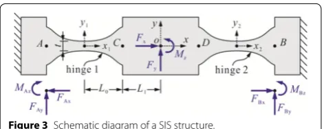
Structure I-III can be schematically illustrated in Fig-ure 3. It is obvious that static indeterminacy causes axial tension in lateral deformations, resulting in nonlinear load-deflection relationship. However, the deflection of a flexure-based mechanism is very small when compared to the dimension of the mechanism. Thus, the above structural nonlinearity can be treated as negligible [25]. This is also adopted in this paper.
The reaction forces and moments of the SIS structure are defined in Figure 3. The static equilibrium conditions lead to the following equations:
There are six unknown variables in the above equa-tions. For this statically indeterminate problem, the reac-tions of the structure can be solved using the flexibility method. If we remove the constraints from point B and treat the reactions FBx, FBy, and MBz as additional loads, the original statically indeterminate structure can be transformed into a statically determinate structure. The transformed structure is equivalent to the original ture only when the deflections of the transformed struc-ture at point B are the same as the original structure. As a result, another three equations are derived:
(7) uB vB θB =
P1 0 0
0 E
κGP1+L 2
0P2+P3 L0P2
0 L0P2 P2
Fx Fy Mz =C Fx Fy Mz , (8)
Fx−FAx+FBx=0, Fy+FAy+FBy=0,
Mz−MAz+MBz−(FAy−FBy)(2L0+L1)=0.
where L01 = L0+L1.
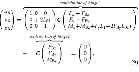
Linear superposition is used to facilitate the calcu-lation, and contribution of hinge 1 (or 2) refers to the deflections of point B when only hinge 1 (or 2) is treated as flexible. Utilizing Eqs. (8) and (9), we obtain the reac-tion forces and moments as below:
Similarly, we can obtain the deflections at point O using the linear superposition method, as shown below:
Subsequently, the in-plane stiffness of the SIS structure can be derived from Eq. (11):
where kL, kT and kR are the longitudinal, transverse, and angular stiffness, respectively.
Substituting P1‒P3 into Eq. (12), the in-plane stiffness of Structure I-III are obtained and provided in Table 1. It is found that the difference between the longitudi-nal and transverse stiffness is over 350 times. Therefore, these structures can be treated as rigid in the longitudi-nal direction. Table 1 also shows that Structure III is very
(9) uB vB θB =
contribution of hinge1
� �� �
1 0 0 0 1 2L01 0 0 1
C
Fx+FBx Fy+FBy
Mz+MBz+FyL1+2FByL01)
+
contribution of hinge2 � �� � C FBx FBy MBz = 0 0 0 , (10)
FAx = 12Fx, FBx= −12Fx,
FAy= −12Fy+ 12 E L01P2
κG P1+L201P2+P3 Mz,
FBy= −12Fy− 12 E L01P2
κG P1+L201P2+P3 Mz,
MAz= L20Fy+ 12 E
κG P1−L0L01P2+P3
E
κG P1+L201P2+P3 Mz,
MBz= L20Fy− 12 E
κG P1−L0L01P2+P3
E
κG P1+L201P2+P3 Mz.
(11) uO vO θO = 1 0 0 0 1 l1
0 0 1
C
Fx+FBx
Fy+FBy
Mz+MBz+Fyl1+2FByL01
= P1
2 0 0
0 E κG P1+P3
2 0
0 0 (
E
κG P1+P3)P2
2[ E
κG P1+L201P2+P3] Fx Fy Mz . (12)
kL =Fx�uO=2�P1,
kT =Fy�vO=2� �κGE P1+P3�, kR=Mz�θO=2�P2+kTL201,
stiff in the longitudinal and transverse directions. Thus, Structure III can be treated as an ideal revolute joint.
3.3 Stress Concentration of the SIS Structure
In Section 3.2, an SIS structure can be treated as rigid in the longitudinal direction. Thus, the normal stress caused by the axial load is not investigated herein. Dur-ing the lateral deformations, the normal stress caused by the bending effect is the dominant stress. Thus, the maxi-mum stress locates on the outer surface of the hinge. The maximum stress on the outer surfaces can be expressed using the following equation:
where kb is the stress concentration factor for bend-ing, σmax and σn are the actual and nominal maximum stresses, respectively. For the leaf hinges in Structure I and II, the stress concentration has little influence on the bending compliance calculation according to DU’s work [29]. As a result, kb can be set to 1 for Structure I and
II. For circular hinges in Structure III, according to the generalized model established in CHEN’s work [30], the stress concentration factor is calculated to be 1.030.
Due to the symmetry, hinge 1 is selected to calcu-late the maximum stress. Based on Figure 3, the inner moment at position x1 within hinge 1 is
Substituting Eqs. (10)‒(12) into Eq. (14), the relation-ship between Mz(x1) and the SIS structure’s deflections is
In this manipulator, Structure I and II act as pris-matic joints, i.e., θO = 0. In this case, substituting Eqs. (1) and (15) into Eq. (13), the following relationship is established:
(13) σmax(x)= −kbσn(x)= −
kby(x)Mz(x) Iz(x)
= −3kbMz(x) 2dy2(x) ,
(14) Mz(x1)=MAz+FAy(L0+x1), x1∈ [−L0,L0].
(15) Mz(x1)= kT[(L0+L1)θO−vO]x1
2 +
θO
P2, x1∈ [−L0,L0].
(16) σx(x1)
vO
= 3kbkTx1
dt2 , x1∈ [−L0,L0].
Table 1 In‑plane stiffness of the SIS structures
Longitudinal kL /(N/μm)
Transverse kT /(N/μm)
Rotational kR /(N·m/rad)
SIS I 17.49 4.350 × 10⁻² 23.53
SIS II 18.54 5.182 × 10⁻² 26.72
On the other hand, Structure III functions as a revolute joint, and thus vO = 0. Substituting Eqs. (2) and (15) into (13), the relationship between the σx and vO is established:
Eqs. (16) and (17) are utilized to obtain the maximum allowable deflections of the SIS structure. For Structure I and II, Eq. (16) shows that the maximum stress locates at both ends of the hinge. For Structure III, the location of the maximum stress can be obtained by differentiating Eq. (17) to x1. Taking the yield strength of the material into consideration, the maximum allowable deflections of Structure I-III are calculated to be 1.46 mm, 1.30 mm, and 5.349 mrad, respectively.
4 Statics and Dynamics Modeling
Monolithic flexure-based mechanisms exhibit friction-less motions, resulting in an extremely low damping ratio. Hence, the nano-manipulator can be approximated as an undamped system. Based on Lagrange’s equation, the dynamics of a system can be expressed as follows:
where T and V denote the total kinetic and poten-tial energy of the system, respectively; qi and Qi are
the ith generalized coordinate and non-conservative force, respectively; and N is the number of generalized coordinates.
The first three modes of the nano-manipulator are the linear motions in the x- and y-axes and the angular motion about the z-axis. The linear motions in each axis are the primary motions, whereas the angular motion about the z-axis is an unexpected motion degrading the motion accuracy. In this section, the dynamics models in both linear and angular motions are established.
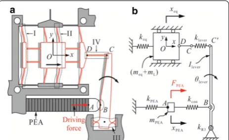
4.1 Influence of the lever’s compliance
The lever in flexure-based mechanisms is typically treated as a rigid element [26, 27, 31] to facilitate the modeling process. This approximation may affect the estimated parameters of the overall system, e.g., the displacement amplification ratio. Figure 4(a) examines the lateral deformations of the lever in the nano-manipulator when a lateral force is applied at the free end. The contribu-tion of Structure III is equivalent to a revolute joint with a torsional stiffness of kR3. If the lever is assumed to be rigid, the free end moves to point C′. However, the lever is flexible, and the actual position of the free end is point
(17)
σx(x1)
θO
= −3kb[kT(L0+L1)P2x1+2]
4dP2
r+t2−r
1−x21
r2
2,
x1∈ [−L0,L0].
(18) d
dt ∂
T ∂q˙i
−∂T
∂qi +∂V
∂qi
=Qi, i=1, 2,. . .,N,
C, with a distance of δ to point C′. The distance δ is neg-ligible in very short levers while it becomes noticeable in long levers. In this paper, the equivalent structure shown in Figure 4(b) is proposed to account for the lever’s com-pliance, where klever is the equivalent lateral stiffness of the lever with “clamped-free” boundary conditions. The modeling of klever is straightforward using the mechanics of materials, and thus it is omitted for the conciseness of this paper. In the lever mechanism, klever is calculated to be 1.111 N/μm.
Figure 5(a) shows the deformation of the manipulator in the x-axis, where linkages 2 and 4 remain stationary, and the central platform, linkages 1 and 3 generate the same displacement. This corresponds to the first/second mode. The masses of the central platform, linkages 1 and 3 are denoted as m0, m1, and m3, respectively. In the con-tact interface, point A is the end of the PEA and point
B represents the contact point on the lever. The lumped mass model in the x-axis can be depicted in Figure 5(b), where mL is the load mass, and Ilever denotes the moment of inertia of the lever. In Figure 5(b), the equivalent
Figure 4 Influence of the lever’s compliance: (a) deformations under a lateral force and (b) the equivalent structure.
stiffness and the effective mass of the central platform are defined in the following equation:
From the static and dynamic point of view, the PEA is equivalent to an active force generator. In Figure 5(b), the equivalent stiffness, the driving force, and the effec-tive mass of the PEA are denoted as kPEA, FPEA, and mPEA, respectively; and kcon represents the equivalent contact stiffness of the contact interface. Further, a dimension-less parameter, η = kcon/kPEA, is proposed to characterize the contact stiffness. Three generalized coordinates are defined in Figure 5(b), namely, the displacement of the PEA (xPEA), the rotation angle of the lever (θlever), and the linear displacement of the central platform (xeq).
In this nano-manipulator, the connection between the PEA and the lever is not firm, and preload force is utilized to keep the PEA and the lever in contact. The input stiffness
kin is defined as the linear stiffness at point B when no PEA
is installed. If kin is too low or the preload force is not large
enough, the detachment phenomenon may occur in large step motions. However, if the input stiffness is too high, the displacement of the PEA will be significantly reduced. Based on Figure 5(b), kin can be calculated as follows:
The output stiffness is the linear stiffness of the central platform in the x or y axis that can be modeled as
The displacement amplification ratio of the lever mech-anism is the ratio between the displacements of points C
and B, which can be expressed as
The influence of the lever’s compliance is significant. If the lever is assumed to be rigid, klever converges to infin-ity. In this case, kin, kout, and kamp will be overestimated. On the contrary, if the lever’s compliance is considered, the modeling complexity will increase significantly. Therefore, a criterion is necessary to to decide whether the lever’s compliance can be neglected or not. Based on Eqs. (20)‒(22), klever can only be neglected if the following two conditions are satisfied:
(19) k
eq=2(kT1+kT2),
meq=m0+m1+m3.
(20) kin= keqklever
keq+klever
·h
2 3 h22+
kR3 h22.
(21) kout=keq+
η
1+ηh22kPEA+kR3
klever η
1+ηh22kPEA+kR3+h23klever .
(22) kamp=
xeq
h2θlever
= h3 h2
· klever klever+keq
.
(23)
klever>100keq,
h23klever>100h22kPEA+kR3.
Eq. (23) is the criterion to decide whether the lever can be treated as rigid or not. In this nano-manipulator,
klever = 11.7keq and h32klever = 0.618(h22kPEA+kR3). As a result, the lever’s compliance must be considered.
4.2 Dynamics of the Nano‑manipulator in the x‑axis
Based on Figure 5(b), the total kinematic and potential energy of the nano-manipulator are given below:
Substituting Eqs. (24) and (25) into Eq. (18), the nano-manipulator’s equations of motion in the x-axis are estab-lished as follows:
where
There are three modal vibrations for the linear motions in the x-axis. The corresponding natural frequencies can be numerically obtained using
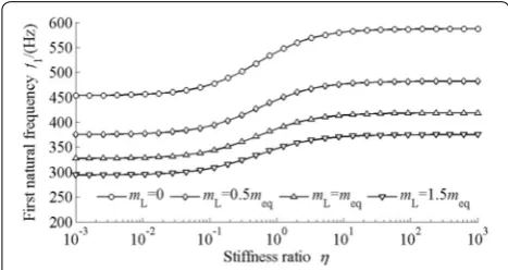
As the nano-manipulator is not designed as a high-speed scanner, only the first natural frequency is inves-tigated, and all the higher order dynamics is neglected. The influence of the contact stiffness and the load mass on the first natural frequency is analyzed and shown in Figure 6. The variation range of η is 10−3 to 103, corre-sponding to the cases of low and high contact stiffness, respectively. When the contact stiffness is low, the first natural frequency converges to its lower bound, cor-responding to the case when no PEA is installed. When the contact stiffness increases, the first natural frequency gradually converges to its upper bound. When η > 100, the first natural frequency starts to converge. This indi-cates that the contact interface can be treated as rigid if
η > 100. As the load mass increases the effective mass of
(24)
T = 12mPEAx˙PEA2 + 12Ileverθ˙ 2 lever+ 12
meq+mLx˙2eq.
(25)
V = 12kPEAx2PEA+12ηkPEA(h2θlever−xPEA) 2
+ 12kR3θlever2 +12klever
h3θlever−xeq2+12keqxeq2.
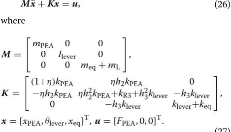
(26)
Mx¨+Kx=u,
(27)
M=
mPEA 0 0
0 Ilever 0
0 0 meq+mL
,
K =
(1+η)kPEA −ηh2kPEA 0 −ηh2kPEA ηh22kPEA+kR3+h23klever −h3klever
0 −h3klever klever+keq
,
x= [xPEA,θlever,xeq]T, u= [FPEA, 0, 0]T.
(28)
K−
2πfi2M
the nano manipulator, its influence is also obvious in Fig-ure 6: the first natural frequency decreases when the load mass increases.
4.3 Static Analysis of the Nano‑manipulator
In static modeling, the velocities and accelerations are zero. Substituting these into Eq. (26), we can solve for the static relationships between the outputs and the input of the nano-manipulator, as shown below:
where xPEA0 = FPEA/kPEA is defined as the nominal dis-placement of the PEA (free extension without loads).
In order to investigate the influence of the contact stiff-ness on the nano-manipulator’s static characteristics, the following three dimensionless ratios are introduced to characterize the actual displacement of the PEA, the dis-placement applied to the lever, and the disdis-placement of the central platform, respectively:
As Figure 7 illustrates, if the contact stiffness is low,
g1 converges to its upper bound of 1, and both g2 and g3 converge to zero. As a result, the majority of the PEA’s displacement is not transmitted to the lever, but sumed in the contact interface. In contrast, if the con-tact stiffness is high, both g1 and g2 converge to kPEA/ (kin+kPEA), and g3 converges to its upper bound of
kPEAkamp/(kin+kPEA). Therefore, in practice, it is desirable to improve the contact stiffness so as to achieve larger workspace.
4.4 Angular Motion of the Nano‑manipulator
As illustrated in Figure 8(a), when a moment Mz is applied on the central platform, the central platform and all the linkages experience almost the same rotations,
(29)
xPEA= kin+ηkPEA
kin+η(kin+kPEA)·xPEA0, θlever= kin+η(kηkPEAin+kPEA) ·
xPEA0
h2 ,
xeq= kin+ηkη(kPEAink+ampkPEA) ·xPEA0.
(30)
g1(η)=
xPEA
xPEA0
,g2(η)=
h2θlever
xPEA0
,g3(η)=
xeq
xPEA0
.
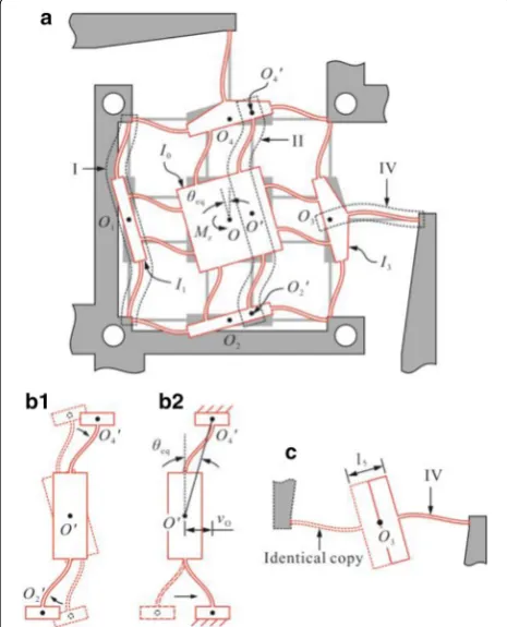
denoted as θeq. Figure 8(a) actually shows the third mode of the nano-manipulator. Based on the computational analysis, the lever mechanisms are almost stationary. Thus, this angular motion of the central platform has no effect on the PEAs, and the installations of the PEAs will not affect the angular behavior of the central platform.
The effective moment of inertia of the central platform, linkages 1 and 3 are denoted as I0, I1, and I3, respectively. The corresponding rotation centers of linkages 1‒4 are labeled as Oi (i = 1‒4). During the angular motion, the
load mass will increase the central platform’s moment of inertia. If the load mass is assumed to be distributed uniformly across the central platform, the total kinematic energy of the nano-manipulator can be written as
where IL≈mLI0/m0 is the moment of inertia of the load mass.
For Structure I, the deformation is a rotation about the
z-axis. The deformation of Structure II is separated and illustrated with dashed lines in Figure 8(b1). The respec-tive rotation centers are labeled as O′, O2′, and O′4. Since the leaf springs and linkages are connected in parallelo-gram configurations, during the angular motion, the dis-tance between points O′ and O′4 is constant and equal to the distance between points O and O4:
In Figure 8(b1), solid lines show a transformed struc-ture obtained by counter rotating Strucstruc-ture II by an angle of −θeq. A further transformation is illustrated in Fig-ure 8(b2): flipping the deformation of the lower flexure hinge. The above operations do not change the potential energy of Structure II. Thus, the angular deformation of Structure II is transformed to a linear deformation vO. The relationship between vO and θeq can be established based on the geometric constraints as below:
(31) T = 1
2[I0+IL+2(I1+I3)]θ˙
2 eq,
(32)
O′O′4= |OO4| =(t3+2l2+l3)2.
(33)
vO=
O′O′4·sinθeq≈ |OO4|θeq.
Figure 6 Influence of η and mL on the first natural frequency.
As illustrated in Figure 8(a), Structure IV rotates about point O3 during the angular motion. If an identical copy of Structure IV is connected to the opposite side, a new structure is obtained, as shown in Figure 8(c). The topology of the new structure is the same as SIS I. The
deformation is an angular displacement of θeq about the
z-axis.
Based on the above analyses, the total potential energy of the nano-manipulator is derived as follows:
where k′
R4 is the angular stiffness of the new structure in Figure 8(c). In this manipulator, l5 = 12.32 mm. Utilizing Eq. (12), we have k′
R4 = 7.272 N·m·rad−1. Substituting Eqs. (31) and (34) into Eq. (18), the nano-manipulator’s equations of motion about the z-axis is established to be
Accordingly, the third natural frequency of the nano-manipulator can be calculated using
5 Experimental Verification 5.1 Experimental Setups
The static and dynamic characteristics of the nano-manipulator are experimentally investigated to verify the established models. Figure 9(a) shows the experimen-tal setup for the static test, where the applied force and the resultant displacement of the central platform are measured. This corresponds to the output stiffness. The applied force is measured by a force gauge (HF-10 from
(34)
U=4kR1θeq22+kT2|OO4|θeq2
2+kR4′ θeq22
=4kR1+4kT2|OO4|2+kR4′
θeq2
2,
(35)
[I0+IL+2(I1+I3)]θ¨eq
+ 4kR1+4kT2|OO4|2+kR4′
θeq=Mz.
(36) f3= 1
2π
4kR1+4kT2|OO4|2+kR4′ I0+IL+2(I1+I3)
.
Figure 8 Angular motion of the nano‑manipulator: (a) overall defor‑ mation, (b1) and (b2) equivalent transformations of Structure II, and (c) transformation of Structure IV.
ALGOL), and the displacement is measured using a dis-placement probe (GT21 from TESA Technology). Fig-ure 9(b) shows the experimental setup for the dynamic test, where a modal hammer (ENDEVCO 2301-10 from MEGGITT) is used to excite the nano-manipulator, and the response is measured by two accelerometers (4507B from Brüel & Kjær) installed on the central platform.
During the experimental tests, the parameters of the nano-manipulator with and without the PEAs installed are measured individually. In the installations of the PEAs, each PEA is bolt-fixed on the nano-manipulator, and the preload force is manually adjusted. Based on the previous analyses, higher contact stiffness is preferred during the installation. The load mass is not measured in the static test because it has no influence on the static parameters of the nano-manipulator. In the dynamic test, the load mass is measured to be 53.4 g, including the fix-tures and two accelerometers.
5.2 Statics of the Nano‑manipulator
The measured and estimated output stiffness of the nano-manipulator are listed in Table 2. If no PEA is not installed, the analytical results are obtained by substitut-ing kPEA = 0 and η = 0 into Eq. (21). In this case, the esti-mation error of the analytical model (Analytical 1) is only −2%. If the PEAs are installed, the output stiffness of the nano-manipulator increases. As η is an unknown vari-able, the lower and upper bounds of the analytical results are provided. The measured output stiffness in each axis is close to the upper bound of the analytical results, indi-cating that high contact stiffness is achieved.
In order to investigate the influence of the lever’s com-pliance, the analytical results with rigid lever assumption (Analytical 2) are also presented in Table 2 for the com-parison. These analytical results are obtained by assign-ing klever a large value according to the criterion defined in Eq. (23). When no PEA is installed, the estimation error with rigid lever assumption is 42%. Such a high overestimation is not acceptable.
5.3 Dynamics of the Nano‑manipulator
The frequency responses of the nano-manipulator are presented in Figure 10. Only the experimental results in the x-axis are presented due to the symmetry of the nano-manipulator. There are three peaks in the magnitude plot.
The first peak corresponds to the first (or second) mode and the other two peaks are the unmodeled higher order dynamics. It is clearly illustrated that the installation of the PEAs only increases the first natural frequency.
The first natural frequencies in the x- and y-axes are given in Table 3. Without the PEAs, the first natural frequency in the x-axis is measured to be 320 Hz. If the lever’s compliance is taken into consideration (Analyti-cal 1), the estimation errors in the x-axis is 3.3%. When the PEAs are installed, the first natural frequency in the
x-axis increase to 429 Hz. In this case, the lower and upper bounds of the analytical result are listed in Table 3. The measured first natural frequency is very close to the upper bound of the analytical result. This also demon-strates that high contact stiffness is achieved. Similarly, if the lever is assumed to be rigid (Analytical 2), the mod-eling accuracy is significantly affected. When no PEA is installed, the estimation error is 20.9%.
In current experimental setup, the third mode (rota-tions about the z-axis) doesn’t show up in the measured data. Therefore, the computational analysis is employed to evaluate the nano-manipulator’s behavior during the angular motions. Based on the computational results, the third natural frequency with the 53.4 g load mass is found to be 769.2 Hz. The analytical result is 754.1 Hz, corre-sponding to an estimation error of 2%, and thus validat-ing the analytical model.
Table 2 Output stiffness in the x‑axis
Measured
(N/μm) Analytical 1(N/μm) Analytical 2(N/μm)
No PEA 0.50 0.49 0.71
PEA installed 0.74 0.49‒0.78 0.71‒1.89
Figure 10 Frequency response in the x‑axis.
Table 3 First natural frequencies in the x‑axis
Measured (Hz) Analytical 1 (Hz) Analytical 2 (Hz)
No PEA 320 330.5 387.0
6 Conclusions
1. An XY flexure-based nano-manipulator is presented in this paper. Two PEAs are employed to generate actuations and the cross-axis couplings are attenu-ated in the kinematic chains. The flexure hinges, arranged in SIS configurations, function as prismatic and revolute joints. Lever mechanism is utilized to magnify the displacement of the PEA. It is found that the lever’s compliance may significantly affect the estimated parameters of the nano-manipulator, such as the input/output stiffness and the first natu-ral frequency. In this paper, a criterion is proposed to decide whether the lever’s compliance can be neglected or not. The lever’s compliance can be mod-eled by cascading a linear spring at the end of the lever. Although simple in formulation, this methodol-ogy is effective in improving the modeling accuracy, as verified through experimental results.
2. The dynamics of the nano-manipulator in linear and angular motions is analyzed. The influence of the contact stiffness and the load mass is analyti-cally investigated. Higher contact stiffness results in improved performances, such as larger workspace and higher first natural frequency. The influence of the load mass is also significant as it adds extra iner-tia to the nano-manipulator.
3. The nano-manipulator is monolithically fabricated using wire electrical discharge machining technique. During the installation of the PEAs, the preload forces of the PEAs are manually tuned for a high con-tact stiffness. The analytical results show good mod-eling accuracy in comparison with the experimental results, and thus verifying the established models. The methodologies proposed in this paper are appli-cable in the design and optimization of flexure-based mechanisms.
Authors’ contributions
YDQ designed the prototype, carried out the experiments and wrote the paper. XZ participated in the revision of the paper. BS participated in the design of experiments and revision of the paper. YLT and DWZ participated in the mechical design and manufacture of the prototype. All authors read and approved the final manuscript.
Author details
1 Institute of Robotics and Automatic Information System (Tianjin Key Laboratory of Intelligent Robotics), Nankai University, Tianjin 300350, China. 2 Robotics and Mechatronics Research Laboratory, Department of Mechanical and Aerospace Engineering, Monash University, Clayton, VIC 3800, Australia. 3 School of Mechanical Engineering, Tianjin University, Tianjin 300072, China.
Authors’ Information
Yan‑Ding Qin is currently an associate professor at Institute of Robotics and Automatic Information System, Nankai University, China. He received his PhD degree from Tianjin University, China, in 2012. His research interests include micro/nano manipulation and 3D bio‑printing.
Xin Zhao is currently a professor at Institute of Robotics and Automatic Information System, Nankai University, China. He received PhD degree from
Nankai University, China, in 1997. His research interests include micro operation robotics, MEMS, and biological pattern and tissue formation.
Bijan Shirinzadeh is currently a professor at Department of Mechanical and Aerospace Engineering, Monash University, Australia. He received his PhD degree from The University of Western Australia, Australia, in 1990. His research interests include micro/nano manipulation, systems kinematics and dynamics, haptics and robotic‑assisted surgery and microsurgery, and advanced manufacturing. Yan‑Ling Tian is currently a professor at School of Mechanical Engineering, Tianjin University, China. He received his PhD degree from Tianjin University, China, in 2005. His research interests include micro/nano manipulation, mechanical dynamics, surface metrology and characterization
Da‑Wei Zhang is currently a professor at School of Mechanical Engineering, Tianjin University, China. He received his PhD degree from Tianjin Univer-sity, China, in 1995. His research interests include micro/nano positioning techniques, high speed machining methodologies, and dynamic design of machine tools.
Acknowledgements
Supported by National Natural Science Foundation of China (Grant Nos. 61403214, 61327802, U1613220), and Tianjin Provincial Natural Science Foun‑ dation of China (Grant Nos. 14JCZDJC31800, 14JCQNJC04700).
Competing interests
The authors declare that they have no competing interests.
Ethics approval and consent to participate Not applicable.
Publisher’s Note
Springer Nature remains neutral with regard to jurisdictional claims in pub‑ lished maps and institutional affiliations.
Received: 27 April 2016 Accepted: 14 January 2018
References
1. D H Wang, Q Yang, H M Dong. A monolithic compliant piezoelectric‑ driven microgripper: design, modeling, and testing. IEEE/ASME Transac-tions on Mechatronics, 2013, 18(1): 138‑147.
2. Y Qin, B Shirinzadeh, Y Tian, et al. Design issues in a decoupled XY stage: static and dynamics modeling, hysteresis compensation, and tracking control. Sensors and Actuators A: Physical, 2013, 194: 95‑105.
3. T Secord, H H Asada. A variable stiffness PZT actuator having tunable resonant frequencies. IEEE Transactions on Robotics, 2010, 26(6): 993‑1005. 4. H Tang, Y Li. Design, analysis, and test of a novel 2‑DOF nanopositioning
system driven by dual mode. IEEE Transactions on Robotics, 2013, 5. H Liu, J Wen, Y Xiao, et al. In situ mechanical characterization of the cell
nucleus by atomic force microscopy. ACS Nano, 2014, 8(4): 3821‑3828. 6. Y Qin, Y Tian, D Zhang, et al. A novel direct inverse modeling approach for
hysteresis compensation of piezoelectric actuator in feedforward applica‑ tions. IEEE/ASME Transactions on Mechatronics, 2013, 18(3): 981‑989. 7. M Pellegrino, P Orsini, M Pellegrini, et al. Integrated SICM‑AFM‑optical
microscope to measure forces due to hydrostatic pressure applied to a pipette. Micro and Nano Letters, 2012, 7(4): 317‑320.
8. S Ryu, R Kawamura, R Naka, et al. Nanoneedle insertion into the cell nucleus does not induce double‑strand breaks in chromosomal DNA. Journal of Bioscience and Bioengineering, 2013, 116(3): 391‑396. 9. K Kuhnen. Modeling, identification and compensation of complex hys‑
teretic and log(t)‑type creep nonlinearities. Control and Intelligent Systems, 2005, 33(2): 134‑147.
10. W T Ang, P K Khosla, C N Riviere. Feedforward controller with inverse rate‑ dependent model for piezoelectric actuators in trajectory‑tracking appli‑ cations. IEEE/ASME Transactions on Mechatronics, 2007, 12(2): 134‑142. 11. M Szymonski, M Targosz‑Korecka, K E Malek‑Zietek. Nano‑mechanical
12. F Iwata, M Adachi, S Hashimoto. A single‑cell scraper based on an atomic force microscope for detaching a living cell from a sub‑ strate. Journal of Applied Physics, 118, 134701 (2015), http://dx.doi. org/10.1063/1.4931936.
13. J M Paros, L Weisbord. How to design flexure hinges. Machine Design, 1965, 37(27): 151‑156.
14. Y Li, Q Xu. Development and assessment of a novel decoupled XY paral‑ lel micropositioning platform. IEEE/ASME Transactions on Mechatronics, 2010, 15(1): 125‑135.
15. H C Liaw, B Shirinzadeh, J Smith. Robust neural network motion tracking control of piezoelectric actuation systems for micro/nanomanipulation. IEEE Transactions on Neural Networks, 2009, 20(2): 356‑367.
16. Y Li, Q Xu. Design and analysis of a totally decoupled flexure‑based XY parallel micromanipulator. IEEE Transactions on Robotics, 2009, 25(3): 645‑657.
17. L J Lai, G Y Gu, L M Zhu. Design and control of a decoupled two degree of freedom translational parallel micro‑positioning stage. Review of Scientific Instruments, 2012, 83(4): 045105‑1‑17.
18. B J Kenton, K K Leang. Design and control of a three‑axis serial‑kinematic high‑bandwidth nanopositioner. IEEE/ASME Transactions on Mechatronics, 2012, 17(2): 356‑369.
19. Y K Yong, T F Lu, D C Handley. Review of circular flexure hinge design equations and derivation of empirical formulations. Precision Engineering, 2008, 32(2): 63‑70.
20. Y Li, Q Xu. Modeling and performance evaluation of a flexure‑based XY parallel micromanipulator. Mechanism and Machine Theory, 2009, 44(12): 2127‑2152.
21. W O Schotborgh, F G M Kokkeler, H Tragter, et al. Dimensionless design graphs for flexure elements and a comparison between three flexure elements. Precision Engineering, 2005, 29(1): 41‑47.
22. H C Liaw, B Shirinzadeh. Enhanced adaptive motion tracking control of piezo‑actuated flexure‑based four‑bar mechanisms for micro/nano manipulation. Sensors and Actuators A: Physical, 2008, 147(1): 254‑262. 23. Q Yao, J Dong, P M Ferreira. Design, analysis, fabrication and testing of
a parallel‑kinematic micropositioning XY stage. International Journal of Machine Tools & Manufacture, 2007, 47(6): 946‑961.
24. Q Xu. New flexure parallel‑kinematic micropositioning system with large workspace. IEEE Transactions on Robotics, 2012, 28(2): 478‑491.
25. Y Qin, B Shirinzadeh, D Zhang, et al. Compliance modeling and analysis of the statically indeterminate symmetric flexure structure. Precision Engineering, 2013, 37(2): 415‑424.
26. S B Choi, S S Han, Y M Han, et al. A magnification device for precision mechanisms featuring piezoactuators and flexure hinges: Design and experimental validation. Mechanism and Machine Theory, 2007, 42(9): 1184‑1198.
27. Q Xu, Y Li, N Xi. Design, fabrication, and visual servo control of an XY parallel micromanipulator with piezo‑actuation. IEEE Transactions on Auto-mation Science and Engineering, 2009, 6(4): 710‑719.
28. Y Qin, B Shirinzadeh, Y Tian, et al. Design and computational optimization of a decoupled 2‑DOF monolithic mechanism. IEEE/ASME Transactions on Mechatronics, 2014, 19(3): 872‑881.
29. S W Han, H K Shin, S H Ryu, et al. Evaluation of DNA transcription of living cell during nanoneedle insertion. Journal of Nanoscience and Nanotech-nology, 2016, 16(8): 8674‑8677.
30. A J Mcdaid, K C Aw, S Q Xie, et al. Optimal force control of an IPMC actu‑ ated micromanipulator for safe cell handling. Proceedings of the Proceed-ings of SPIE - The International Society for Optical Engineering, F, 2012. 31. Y Tian, B Shirinzadeh, D Zhang. A flexure‑based five‑bar mechanism for