R E S E A R C H
Open Access
Bayesian group sparse learning for music
source separation
Jen-Tzung Chien
*and Hsin-Lung Hsieh
Abstract
Nonnegative matrix factorization (NMF) is developed for parts-based representation of nonnegative signals with the sparseness constraint. The signals are adequately represented by a set of basis vectors and the corresponding weight parameters. NMF has been successfully applied for blind source separation and many other signal processing systems. Typically, controlling the degree of sparseness and characterizing the uncertainty of model parameters are two critical issues for model regularization using NMF. This paper presents theBayesian group sparse learningfor NMF and applies it for single-channel music source separation. This method reconstructs the rhythmic or repetitive signal from a common subspacespanned by the shared bases for the whole signal and simultaneously decodes the harmonic or residual signal from anindividual subspaceconsisting of separate bases for different signal segments. ALaplacian scale mixturedistribution is introduced for sparse coding given a sparseness control parameter. The relevance of basis vectors for reconstructing two groups of music signals is automatically determined. A Markov chain Monte Carlo procedure is presented to infer two sets of model parameters and hyperparameters through a sampling procedure based on the conditional posterior distributions. Experiments on separating single-channel audio signals into rhythmic and harmonic source signals show that the proposed method outperforms baseline NMF, Bayesian NMF, and other group-based NMF in terms of signal-to-interference ratio.
Keywords: Bayesian sparse learning; Signal reconstruction; Subspace approach; Group sparsity; Nonnegative matrix factorization; Single-channel source separation
1 Introduction
Many problems in audio, speech and music processing can be tackled through matrix factorization. Different cost functions and constraints may lead to different factorized matrices. This procedure can identify underlying sources from the mixed signals through blind source separation [1]. Nonnegative matrix factorization (NMF) is designed to find an approximate factorizationX ≈ ASfor a data matrixXinto a basis matrixAand a weight matrixSwhich are all nonnegative [2]. Some divergence measures have been proposed to derive solutions to NMF [3,4]. NMF provides a useful learning tool for clustering as well as for classification. When a portion of labeled data are available, the semi-supervised NMF was developed for an improved classification system [5]. Different from standard principal component analysis (PCA) and independent component
*Correspondence: [email protected]
Department of Electrical and Computer Engineering, National Chiao Tung University, Taiwan 30010, Republic of China
analysis (ICA), NMF only allows additive combination due to the nonnegative constraints on matricesAandS. Nev-ertheless, nonnegative PCA and nonnegative ICA were proposed for blind source separation in the presence of nonnegative image and music sources [6].
On the other hand, NMF conducts a parts-based sparse representation where only a few components or bases are relevant for representation of input nonnegative matrixX. The sparseness constraint is imposed in objective func-tion [2]. An automatic relevance determinafunc-tion (ARD) scheme [7-9] is developed to determine relevant bases for sparse representation. Such sparse coding is efficient and robust. However, controlling the sparseness or smooth-ness is influential for system performance. Bayesian learn-ing is beneficial to deal with sparse representation [9] and model regularization [7]. In [10], Bayesian learning was performed for sparse representation of image data where Laplacian distribution was used as prior density. The1
-regularized optimization was comparably performed. In addition, the group-based NMF [11] was proposed to
capture the intra-subject variations and the inter-subject variations in EEG signals. In [12], the group sparse NMF was proposed by minimizing the Itakura-Saito divergence betweenX andAS. In [13], NMF was applied for drum source separation where the factorized components were partitioned into rhythmic sources and harmonic sources. No Bayesian learning was performed in [11-13].
More recently, a Bayesian NMF approach [14] was pro-posed for model selection and image reconstruction. This approach inferred NMF model by a variational Bayes method and a Markov chain Monte Carlo (MCMC) algo-rithm. In [15], a Bayesian NMF with gamma priors for source signals and mixture weights was implemented through a MCMC algorithm. In [16], the Bayesian NMF with Gaussian likelihood and exponential prior was con-structed for image feature extraction where the posterior distribution was approximated by Gibbs sampling proce-dure. In [17], a Bayesian approach for blind separation of linear mixtures of sources was developed. The Stu-dent t distribution for mixture weights was introduced to achieve sparse basis representation. The underde-termined noisy mixtures were separated. However, the case of nonnegative source was not applied. Besides, single-channel source separation is known as an underde-termined problem. In [18], the harmonic structure infor-mation was adopted to estimate the demixed instrumental sources. In [19], the NMF was applied for single-channel speech separation where the speech of target speaker over that of masking speaker was enhanced by using sparse dictionaries learned on a phoneme level for individual speakers.
This paper addresses the problem of underdetermined source separation based on NMF for an application to music source separation [20]. The uses of NMF and Bayesian theory to source separation are not new since they have been many papers [11-13,15]. But, to our best knowledge, the novelty of this paper is to propose Bayesian group sparse (BGS) learning using Laplacian distributionandLaplacian scale mixture(LSM) distribu-tionand apply it for single-channel music signal separa-tion. We present a group-based NMF where the groups of common bases and individual bases are estimated for blind separation of rhythmic sources and harmonic sources, respectively. Bayesian sparse learning is devel-oped by introducing LSM distributions as the priors for two groups of reconstruction weights. Gamma pri-ors are used to represent two groups of nonnegative basis components. The BGS-NMF algorithm is accord-ingly established. A MCMC algorithm is derived to infer BGS-NMF parameters and hyperparameters according to full Bayesiantheory. The rhythmic sources and harmonic sources are reconstructed through the relevant bases in common subspace and individual subspace, respectively. In the experiments, the proposed BGS-NMF is evaluated
and compared with the other NMF methods for single-channel separation of audio signals into rhythmic signals and harmonic signals. From comparative study, we find that the improvement of separation performance bene-fits from Bayesian modeling, group basis representation, and sparse signal reconstruction. Sparser priors identify fewer but more relevant bases and correspondingly lead to a better performance in terms of signal-to-interference ratio.
The remaining of this paper is organized as follows. In the next section, the related studies on NMF and group basis representation are surveyed. Some Bayesian learn-ing approaches are addressed. Section 3 highlights on the construction of BGS-NMF model as well as the infer-ence procedure based on MCMC algorithm. The condi-tional posterior distributions of different parameters and hyperparameters are derived in the sampling procedure. Section 4 reports a series of experiments on underde-termined music source separation with different music sources. The convergence condition in MCMC sampling is investigated. The evaluation of demixed signals in terms of signal-to-interference ratio is reported. Finally, the con-clusions drawn by this study are provided in Section 5.
2 Background survey
In what follows, nonnegative matrix factorization (NMF) and its extensions to different regularization functions are introduced. Several approaches to group basis representa-tion are addressed. Group sparse coding is surveyed. Then Bayesian learning methods for matrix factorization and other related tasks are introduced.
2.1 Nonnegative matrix factorization
NMF is a linear model where the observed signals, fac-torized signals, and source signals are all assumed to be nonnegative. Given a data matrixX = {Xik}, NMF
esti-mates two factorized matricesA = {Aij}andS = {Sjk}
by minimizing the reconstruction error between X and AS. In [2], the sparseness constraint was imposed on min-imization of an objective functionF which is based on a regularized error function
X−AS2+ηa
i
j
f(Aij)+ηs
j
k
f(Sjk) (1)
where ηa ≥ 0 and ηs ≥ 0 are regularization
parame-ters and different sparseness measures could be used, e.g., f(Sjk) = Sjk, f(Sjk) = Sjk, f(Sjk) = Sjkln(Sjk), etc.
Several extensions of NMF have been proposed. In [21], the nonnegative matrix partial co-factorization (NMPCF) was proposed for rhythmic source separation. Given the magnitude spectrogram as input data matrixX, NMPCF decomposes the music signal into a drum or rhythmic part and a residual or harmonic partX ≈ ArSr+AhSh
weight matrix for rhythmic source {Ar,Sr} and for
har-monic source{Ah,Sh}. The prior knowledge from
drum-only signalY ≈ArSrgiven the same rhythmic basesAris
incorporated in joint minimization of two Euclidean error functions
X−ArSr−AhSh2+ηY−ArSr2 (2)
where ηis a trade-off between the first and the second reconstruction errors due toXandY, respectively. In [22], the mixed signals were divided intoLsegments. Each seg-ment X(l) is decomposed into common and individual parts which reflect the rhythmic and harmonic sources, respectively. The common basesArare shared for
differ-ent segmdiffer-ents due to high temporal repeatability in rhyth-mic sources. The individual bases A(l)h are separate for individual segmentldue to the changing frequency and low temporal repeatability. The resulting objective func-tion consists of a weighted Euclidean error funcfunc-tion and the regularization terms due to basesAr andA(l)h which
are expressed by
L
l=1
ω(l)X(l)−ArS(l)r −A(l)h S (l)
h 2+ηLAr2+η
L
l=1
A(l)h 2
(3)
where {ω(l),S(l)r ,S(l)h } denotes the segment-dependent
weights and weight matrices for common basis and indi-vidual basis, respectively. This is a NMPCF for L seg-ments. The solutions to these NMFs are derived and implemented by the multiplicative update rules so that nonnegative constraints are met for individual model parameters. For example, the terms in gradient of objec-tive functionF with respect to nonnegative parameterA are divided into positive terms and negative terms ∂∂AF = ∂F
∂A +
−∂F ∂A
−
where∂∂AF+ > 0 and∂∂AF− > 0. The multiplicative update rule is yielded by
A←A⊗
∂F ∂A
−
∂F ∂A
+
(4)
where⊗anddenote element-wise multiplication and division, respectively.
2.2 Group basis representation
The signal reconstruction methods in (2) and (3) cor-respond to the group basis representation where two groups of basesAr and A(l)h are applied. The separation
of single-channel mixed signal into two source signals is achieved. The issue of underdetermined source separation is resolved. In [11], the group-based NMF (GNMF) was developed by conducting group analysis and construct-ing two groups of bases. The intra-subject variations for a subject in different trials and the inter-subject variations for different subjects could be compensated. Given the
Lsubjects or segments, thelth segment is generated by X(l) ≈ A(l)r S(l)r +A(l)h S
(l)
h whereA (l)
r denotes the common
bases which capture the intra and inter-subject variations and A(l)h denotes the individual bases which reflect the residual information. In general, different common bases A(l)r should be close together since these bases represent
the shared information in mixed signal. Contrarily, indi-vidual bases A(l)h characterize individual features which should be discriminated and mutually far apart [11]. The object function of GNMF is formed by
L
l=1
X(l)−A(l)r S(l)r −A(l)h Sh(l)2+ηa L
l=1
A(l)r 2
+ηa L
l=1
A(l)h 2
+ηar L
l=1 L
m=1
A(l)r −A(m)r 2
−ηah L
l=1 L
m=1
A(l)h −A(m)h 2.
(5)
In (5), the second and third terms are seen as the2 regu-larization functions, the fourth term enforces the distance between different common bases to be small, and the fifth term enforces the distance between different individual bases to be large. Regularization parameters{ηa,ηar,ηah}
are used. The NMPCFs in [21,22] and GNMF in [11] did not consider sparsity in group basis representation.
More generally, a group sparse coding algorithm [23] was proposed for basis representation of group instances {Xk,k∈G}where objective function is defined by
k∈G
Xk−
|D|
j=1
SkjAj
2
+η
|D|
j=1
Sj. (6)
All the instances within a group G share the same dictionaryDwith basis vectors{Aj}|j=D|1. The weight matrix
{Sj}|jD=|1consists of nonnegative vectorsSj=[S1j,. . .,S
|G|
j ]T.
The weight parameters {Sjk} are estimated for different group instances k ∈ G using different bases j ∈ D. In (6), 1 regularization term is incorporated to carry out group sparse coding. The group sparsity was fur-ther extended to structural sparsity for dictionary learning and basis representation. Nevertheless, nonnegative con-straints were not imposed on bases {Aj} and observed
signals{Xk}. Basically, all the above-mentioned methods
2.3 Bayesian learning approaches
Model regularization is critical for improving the gener-alization of a learning machine to new data [7]. Conduct-ing Bayesian learnConduct-ing shall compensate the variations of the estimated parameters and accordingly improve model regularization. Typically, NMF and group basis represen-tation are viewed as learning machine which is based on a set of bases. Following the perspective of relevance vec-tor machines [8,9], Bayesian sparse learning is beneficial to identify relevant bases for regularized basis represen-tation. To do so, sparse priors based on Studentt distri-bution [17] and Laplacian distridistri-bution [10,25] could act as regularization functions and merged with likelihood func-tion to come up witha posterioriprobability. Maximizing the logarithm ofa posteriori probability is equivalent to minimizing the1-regularized error function if Laplacian
prior is applied. Hyperparameters of sparse priors are then used as the regularization parameter which controls the trade-off between a reconstruction error function and a sparsity-favorable penalty function.
In the literature, a probabilistic matrix factorization (PMF) [26] forX=ATSwas proposed by assuming Gaus-sian noise for each independent entry of data matrixX = {Xik}byp(X|A,S,α)= Ni=1 kM=1N(Xik|ATi Sk,α−1)and
assuming Gaussian priorsp(A|αa) = Ni=1N(Ai|0,αa−1I)
andp(S|αs) = Mk=1N(Sk|0,α−s1I)where{α,αa,αs}is a
set of precision parameters of Gaussians. Here,Aidenotes
the ith column ofA andSk denotes the kth column of
S. Learning for PMF is equivalent to maximizing the log posterior likelihood
lnp(A,S|X,α,αa,αs)=lnp(X|A,S,α)
+lnp(A|αa)+lnp(S|αs)+C (7)
with respect to A and S. In (7), C is a constant. This optimization turns out to minimizing the sum-of-squares error function with quadratic regularization terms
N
i=1 M
k=1
(Xik−ATi Sk)2+ηa N
i=1
Ai2+ηs M
k=1
Sk2. (8)
The regularization terms are determined from hyperpa-rameters byηa = αa/αandηs = αs/α. Bayesian learning
of PMF was performed through MCMC algorithm where Gaussian-Wishart priors for Gaussian mean vectors and precision matrices were assumed. There was no constraint on nonnegative matrices by using PMF. No sparse learning was considered.
In [27], a full Bayesian NMF was implemented to deter-mine the number of bases according to the marginal like-lihood. Furthermore, Bayesian nonparametric approach to NMF was proposed in [28] where model structure was determined through Gamma process NMF. This
method was applied to find both latent sources in spectro-grams and their number. In [25], the group sparse coding [23] was upgraded with Bayesian interpretation. Bayesian sparse learning was only developed for single-sample basis representation. In [29], the group sparse priors were pre-sented for maximum a posteriori estimation of covari-ance matrix which was used in Gaussian graphical model. More recently, the group sparse hidden Markov mod-els (HMMs) [30] were proposed to represent a sequence of observations and have been successfully applied for speech recognition. A set of common bases were shared for representation of speech samples across HMM states, while a set of individual bases were employed to represent speech samples within individual HMM states. Bayesian group sparse learning was performed for speech recog-nition [30] and signal separation [20] by using Laplacian scale mixture distribution.
3 Bayesian group sparse matrix factorization Previous NMF methods [11,13,21] were developed to extract task-specific nonnegative factors, but they did not simultaneously consider the uncertainty of model parameters and control the sparsity of weight parame-ters. In [23,25], the group sparse coding and its Bayesian extension did not imposenonnegativeconstraints in data matrix X and factorized matrices A and S. This paper presents a new Bayesian group sparse learning for NMF (denoted by BGS-NMF) and applied it for single-channel music source separation.
3.1 Model construction
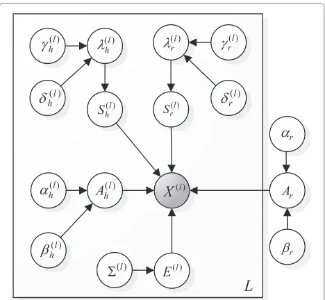
In this study, magnitude spectrogram X = {X(l)} of a mixed audio signal is calculated and chopped intoL seg-ments for implementation of BGS-NMF algorithm. The audio signal is assumed to be mixed from two kinds of source signals. One is rhythmic or repetitive source sig-nal and the other is harmonic or residual source sigsig-nal. As illustrated in Figure 1, BGS-NMF aims to decompose a nonnegative matrixX(l) ∈RN+×Mof thelth segment into a product of two nonnegative matricesA(l)S(l). A linear decomposition model is constructed in a form of
X(l)=ArSr(l)+A(l)h S (l)
h +E(l) (9)
where Ar ∈ RN+×Dr denotes the shared basis matrix for all segments {X(l),l = 1,. . .,L}; A(l)h ∈ RN×Dh
+ and
Figure 1Illustration for group basis representation.There are|D|bases in the dictionary.
to recover the rhythmic signal and the harmonic signal, respectively, from a mixed audio signal. Such a signal recovery problem could be interpreted from a perspec-tive of subspace approach. Namely, an observed signal is demixed into one signal fromprincipal subspacespanned by common bases and the other signal fromminor sub-space spanned by individual bases [31]. Moreover, the sparseness constraint is imposed on two groups of recon-struction weights S(l)r ∈ R D+r×M and S(l)h ∈ R
Dh×M
+ . It is assumed that the reconstruction weights of rhyth-mic sources S(l)r and harmonic sources Sh(l) are
inde-pendent, but the dependencies between reconstruction weights within each group are allowed. Assuming that thekth noise vectorEk(l)is Gaussian distributed with zero mean and N × N diagonal covariance matrix (l) = diag{[(l)]ii}which is shared for all samples within a
seg-mentl, the likelihood function of an audio signal segment X(l)is expressed by
p(X(l)|(l))= N
i=1 M
k=1
N(Xik(l)|[ArS(l)r ]ik
+[A(l)h S(l)h ]ik, [(l)]ii).
(10)
BGS-NMF model is therefore constructed with parame-ters(l)= {Ar,A(l)h ,S
(l)
r ,S(l)h ,(l)}.
3.2 Priors for Bayesian group sparse learning
From Bayesian perspective, the uncertainties of BGS-NMF parameters, expressed by prior densities, are con-sidered to assuremodel regularization. Using BGS-NMF model, the common basesArare constructed to represent
the characteristics of repetitive patterns for different data segments, while the individual bases A(l)h are estimated to reflect unique information in each segmentl. Sparsity control is enforced in the corresponding reconstruction weightsS(l)r andS(l)h so that relevant bases are retrieved for
group basis representation. In accordance with [15], the nonnegative basis parameters are assumed to be gamma distributed by
p(Ar)= N
i=1 Dr
j=1
G([Ar]ij|αrj,βrj) (11)
p(A(l)h )= N
i=1 Dh
j=1
G([A(l)h ]ij|αhj(l),βhj(l)) (12)
where(l)a = {{αrj,βrj},{α(l)hj,βhj(l)}}denotes the hyperpa-rameters of gamma distributions and{Dr,Dh}denote the
numbers of common bases and individual bases, respec-tively. Gamma distribution is an exponential family distri-bution fornonnegative data. Its two parameters{α,β}can be adjusted to fit different shapes of distributions. In (11) and (12), all entries in matricesArandA(l)h are assumed to
be independent.
Importantly, we control the sparsity of reconstruction weights by using prior density based on the Laplacian scale mixture (LSM) distribution [25]. The LSM of a reconstruction weight of common basis is constructed by [Sr(l)]jk=(λ(l)rj)−1u
(l)
rj whereu (l)
rj is a Laplacian distribution
p(u(l)rj )= 12exp{−|u(l)rj|}with scale 1 andλ(l)rj is an inverse scale parameter. Accordingly, the parameter [S(l)r ]jkhas a
Laplacian distribution
p([S(l)r ]jk|λ(l)rj)= λ(l)rj
2 exp{−λ
(l)
rj[S(l)r ]jk} (13)
which is controlled by a positive continuous mixture parameterλ(l)rj ≥0. Considering a gamma distribution for
inverse scale parameter, i.e.,p(λ(l)rj )=G(λrj(l)|γrj(l),δrj(l)), the marginal distribution of a reconstruction weight can be calculated by [25]
p([S(l)r ]jk)=
∞
0
p([S(l)r ]jk|λ(l)rj)p(λ (l) rj)dλ
(l) rj
= γ
(l) rj (δ
(l) rj )
γrj(l)
2(δ(l)rj +[S(l)r ]jk)γ (l)
rj +1 .
In (13) and (14), the constraint [S(l)r ]jk≥ 0 has been
con-sidered. This LSM distribution is obtained by adopting the property that gamma distribution is theconjugate prior for Laplacian distribution. In application of image cod-ing, LSM distribution was estimated and measured to be sparser than Laplacian distribution by approximately a factor of 2 [25]. Figure 2 compares Gaussian, Laplacian, and LSM distributions with specific parameters. In this example, LSM is the sharpest distribution among these distributions. In addition, a truncated LSM prior for nonnegative parameter [Sr(l)]jk∈ R+is adopted, namely,
the distribution of negative parameter is forced to be zero. The sparse prior for reconstruction weight for individual basis [S(l)h ]jk is also expressed by LSM
distri-bution with hyperparameter{γhj(l),δhj(l)}. The
hyperparam-eters of BGS-NMF is formed by (l) = {(l)a ,(l)s =
{γrj(l),δ(l)rj ,γhj(l),δ(l)hj}}. Figure 3 displays a graphical repre-sentation for construction of BGS-NMF with different parameters(l)and hyperparameters(l).
By combining the likelihood function in (10) and the prior densities in (11) to (13), the negative logarithm of posterior distribution −lnp(Ar,A(l)h ,S(l)r ,Sh(l)|X) can
be calculated and arranged as a new objective function expressed by
L
l=1
N
i=1
M
k=1
(Xik(l)−[ArSr(l)]ik−[A(hl)S
(l)
h]ik)2
+ηaL N
i=1
Dr
j=1
((1−αrj)ln[Ar]ij
+βrj[Ar]ij)
+ηa
L
l=1
N
i=1
Dh
j=1
((1−αhj(l))ln[A(hl)]ij
+βhj(l)[Ah(l)]ij)+ηsr
L
l=1
Dr
j=1
M
k=1 [S(rl)]jk
+ηsh
L
l=1
Dh
j=1
M
k=1 [S(hl)]jk
(15)
where {ηa,ηsr,ηsh} denote the regularization parameters for two groups of bases and reconstruction weights. Some BGS-NMF parameters or hyperparameters have been absorbed in these regularization parameters. Com-paring with the objective functions (3) for NMPCF, (5) for GNMF, and (8) for PMF, the optimization of (15) for BGS-NMF shall lead to two groups of signals which are reconstructed from the sparse common basesArand
sparse individual basesA(l)h . The regularization terms due to two gamma bases are additionally considered. Different
-15 -10 -5 0 5 10 15
0 0.1 0.2 0.3 0.4 0.5 0.6
s
p(
s
)
LSM (gamma=0.1,delta=0.1) Laplacian (scale=1) Gaussian (variance=1)
Figure 2Comparison of Gaussian, Laplacian, and LSM distributions.
from the Bayesian NMF (BNMF) [15], BGS-NMF con-ducts group sparse learning which does not only charac-terize the within-segment harmonic information but also represent the across-segment rhythmic regularity. Sparse sets of basis vectors are further determined for sparse rep-resentation. Basically, BGS-NMF follows a general objec-tive function. By applying different hyperparameter values {αrj,βrj,αhj(l),βhj(l)}, probability structures, and prior
distri-butions for{Ar,A(l)h ,S(l)r ,Sh(l)}, BGS-NMF can be realized
to find solutions to NMF [2], NMPCF [21], GNMF [11], PMF [26], and BNMF [15]. Notably, the objective function in (15) is written for comparative study among differ-ent methods. This function only considers BGS-NMF
based on Laplacian prior. BGS-NMF algorithms with Laplacian prior and LSM prior shall be both implemented in the experiments. Nevertheless, in what follows, we address the model inference procedure forBGS-NMF with LSM prior.
3.3 Model inference
The full Bayesian framework for BGS-NMF model based on the posterior distribution of parameters and hyper-parameters p(,|X) is not analytically tractable. A stochastic optimization scheme is adopted. We develop a MCMC sampling algorithm for approximate inference through iteratively generating samples of parameters and hyperparametersaccording to the posterior distri-bution. This algorithm converges by those samples. The key idea of MCMC sampling is to simulate a stationary ergodic Markov chain whose samples asymptotically fol-low the posterior distributionp(,|X). The estimates of parametersand hyperparametersare then computed via Monte Carlo integrations on the simulated Markov chains. For simplicity, the segment indexlis neglected in derivation of MCMC algorithm for BGS-NMF. At each new iterationt+1, the BGS-NMF parameters(t+1)and hyperparameters (t+1) are sequentially sampled in an order of{Ar,Sr,Ah,Sh,,αr,βr,αh,βh,λr,λh,γr,δr,γh,δh}
according to their corresponding conditional pos-terior distributions. In this subsection, we describe the calculation of conditional posterior distributions under BGS-NMF parameters {Ar,Sr,Ah,Sh,}. The
conditional posterior distributions for hyperparame-ters {αr,βr,αh,βh,λr,λh,γr,δr,γh,δh} are derived in the Appendix.
1. Sampling of [Ar]ij. First of all, the common basis
parameter [A(tr+1)]ijis sampled by the conditional
poste-rior distribution
p([Ar]ij|XTi ,(t)Arij,
(t)
Arij)∝p(X
T
i |(t)Arij)p([Ar]ij|
(t) Arij) (16)
where(t)A
rij = {[A
(t+1)
r ]i(1:j−1), [A(t)r ]i(j+1:Dr),S(t)r ,A(t)h ,S(t)h ,
(t)} and (t)A
rij = {α
(t)
rj ,βrj(t)}. Here, Xi denotes the ith
row vector ofX. Notably, for each sampling, we use the preceding bases [A(tr+1)]i(1:j−1) at new iteration t + 1
and subsequent bases [Ar](t)i(j+1:Dr) at current iteration t.
The likelihood function can be arranged as a Gaussian distribution of [Ar]ij
p(XiT|(t)A
rij)∝exp
−([Ar]ij−μ
likel Arij)
2
2[σAlikel
rij ]
2
(17)
whereμlikelA
rij =[σ
likel Arij ]
−2M
k=1([S(t)r ]jkεik(−j)),εik(−j)=Xik− (jm−=11[Ar(t+1)]im[S(t)r ]mk+
Dr m=j+1[A
(t)
r ]im[S(t)r ]mk) − Dh
m=1 [A(t)h ]im[S (t)
h ]mk and [σAlikelrij ]
2=[(t)]
ii (Mk=1
[Sr(t)]jk)−1. By combining likelihood function of (17) and
gamma priorp([Ar]ij|(t)Arij)of (11), the conditional
pos-terior distribution in (16) is derived in a form of
[Ar] α(rjt)−1
ij exp
⎧ ⎨ ⎩−
([Ar]ij−μpostArij)2
2[σApost
rij ]
2
⎫ ⎬
⎭I[0,+∞[([Ar]ij)
(18)
where μpostA
rij = μ
likel Arij − β
(t) rj [σAlikelrij ]
2, [σpost Arij ]
2=[σlikel Arij ]
2,
and I[0,+∞[(z) denotes an indicator function which has
value either 1 ifz ∈[ 0,+∞[ or 0 for the other case. In (18), the posterior distribution for negative [Ar]ijis forced
to be zero. Derivations of (17) and (18) are detailed in the Appendix. However, (18) is not an usual distribution, therefore its sampling requires the use of arejection sam-plingmethod, such as the Metropolis-Hastings algorithm [32]. Using this algorithm, an instrumental distribution q([Ar]ij) is chosen to fit at best the target distribution
(18) so that high rejection condition is avoided or equiv-alently rapid convergence toward true parameter could be achieved. In case of rejection, the previous parame-ter sample is used, namely, [A(tr+1)]ij←[A(t)r ]ij. Generally,
the shape of target distribution is characterized by its mode and width. The instrumental distribution is con-structed as a truncated Gaussian distribution which is calculated by
q([Ar]ij)=N+([Ar]ij|μinstArij, [σ
inst Arij]
2). (19)
In (19), the modeμinstA
rij is obtained by finding the roots of a quadratic equation of [Ar]ij which appears in the
exponent of the posterior distribution in (18). Derivation for the modeμinstA
rij is detailed in the Appendix. In case of complex-valued root or negative-valued root, the mode is forced byμinstA
rij = 0. The width of instrumental distribu-tion is controlled by [σAinst
rij]
2=[σpost
Arij ]
2.
2. Sampling of [Sr]jk. The sampling of reconstruction
weight of common basis [S(tr+1)]jkdepends on the
condi-tional posterior distribution
p([Sr]jk|Xk,(t)Srjk,
(t)
Srjk)∝p(Xk |[Sr]jk,
(t) Srjk)
p([Sr]jk|(t)Srjk)
(20)
where(t)S
rjk = {A
(t+1)
r , [S(tr+1)](1:j−1)k, [Sr(t)](j+1:Dr)k,A(t)h ,
Sh(t),(t)} and(t)srjk = λ
(t)
rj . Xk is the kth column of X.
Again, the preceding weights [S(tr+1)](1:j−1)kat new
iterationtx are used. The likelihood function is rewritten as a Gaussian distribution of [Sr]jkgiven by
p(Xk |[Sr]jk,(t)Srjk)∝exp
⎧ ⎨ ⎩−
([Sr]jk−μlikelSrjk)2
2[σSlikel
rjk ]
2
⎫ ⎬ ⎭. (21)
The Gaussian parameters are obtained by μlikelS
rjk = [σSlikel
rjk ] −2N
i=1([(t)]−ii1[A (t+1)
r ]ijε(ik−j)), εik(−j) = Xik− (jm−=11[A(tr+1)]im[Sr(t+1)]mk+mDr=j+1[A
(t+1)
r ]im[S(t)r ]mk)− Dh
m=1 [A (t) h ]im[S
(t)
h ]mk and [σSlikelrjk ]
2= (N
i=1[(t)]−ii1 ([A(tr+1)]ij)2)−1. Given the Gaussian likelihood and
Laplacian prior, the conditional posterior distribution is calculated by
λ(t)rj exp ⎧ ⎨ ⎩−
([Sr]jk−μpostSrjk )2
2[σSpost
rjk ]
2
⎫ ⎬
⎭I[0,+∞[([Sr]jk) (22)
whereμpostS
rjk =μ
likel Srjk −λ
(t) rj [σSlikelrjk ]
2and [σpost Srjk ]
2=[σlikel Srjk ]
2.
Notably, the hyperparameters {γrj(t+1),δrj(t+1)} in LSM prior are also sampled and used to sample LSM param-eter λ(trj+1) based on a gamma distribution. Here, Metropolis-Hastings algorithm is applied again. The best instrumental distributionq([Sr]jk)is selected to fit (22).
This distribution is derived as a truncated Gaussian dis-tributionN+([Sr]jk|μinstSrjk, [σSinstrjk]2)where the modeμinstSrjk
is derived by finding the root of a quadratic equation of [Sr]jk and the width is obtained by [σSinstrjk]2=[σSpostrjk ]2.
In addition, the conditional posterior distributions for sampling the individual basis parameter [A(th+1)]ijand its
reconstruction weight [S(th+1)]jk are similar to those for sampling [A(tr+1)]ijand [S(tr+1)]jk, respectively. We do not
address these two distributions.
3. Sampling of []−ii1. The sampling of the inverse of noise variance([](tii+1))−1is performed according to the conditional posterior distribution
p([]−ii1|XiT,(t)
ii,
(t) ii)∝p(X
T
i |[]−ii1,(t)ii)p([] −1 ii |(t)ii)
(23)
where (t)
ii = {A
(t+1)
r ,Sr(t+1),Ah(t+1),S(th+1)} and p(
[]−ii1|(t)
ii
= G([]−ii1|αii,βii). The resulting pos-terior distribution can be derived as a new gamma distribution with updated hyperparameters αpost
ii =
M
2 + αii and β
post
ii =
1 2
M
k=1(Xik− Dr
m=1[A (t+1) r ]im
[Sr(t+1)]mk− Dh
m=1[A (t+1) h ]im[S
(t+1)
h ]mk)2 +βii. In the experiments, we conduct MCMC sampling procedure fortmax iterations. However, the firsttmin iterations are
not stable. These burn-in samples are abandoned. The marginal posterior estimates of common basis [Aˆr]ij,
indi-vidual basis [Aˆh]ijand their reconstruction weights [Sˆr]jk
and [Sˆh]jk are calculated by finding the following sample
means, e.g.,
[Aˆr]ij=
1 tmax−tmin
tmax
t=tmin+1
[Ar](t)ij . (24)
With these posterior estimates, the rhythmic source and the harmonic source are calculated by AˆrSˆr and
ˆ
AhSˆh, respectively. The BGS-NMF algorithm is
com-pleted. Different from BNMF [15], the proposed BGS-NMF conducts a group sparse learning based on LSM distribution. Common bases Ar are shared for
different data segmentsl. The group sparse learning per-forms well in our experiments.
4 Experiments
In this study, BGS-NMF is implemented to estimate two audio source signals from a single-channel mixed signal. One source signal contains rhythmic pattern which is con-structed by the bases shared for all audio segments while the other source contains harmonic information which is represented via bases from individual segments. Bayesian sparse learning is performed to conduct probabilistic reconstruction based on the relevant group bases. Some experiments are reported to evaluate the performance of model inference and signal reconstruction.
4.1 Experimental setup
The specification of 44,100-Hz sampling rate and 16-bit resolution was used in the collected audio signals. In our implementation, the magnitude of fast Fourier transform of audio signal was extracted every 1,024 samples with 512 samples in frame overlapping. Each mixed signal was equally chopped into L segments for music source separation. Each segment had a length of 3 s. Sufficient rhythmic signal existed within a segment. The numbers of common bases and individual bases were empirically set to be 15 and 10, respectively, i.e.,Dr = 15 andDh = 10.
The common bases were sufficiently allocated so as to capture the shared base information from different seg-ments. The initial common bases A(r0) and individual
basesA(h0)were estimated by applyingk-means clustering using the automatically detected rhythmic and har-monic segments, respectively. The detection was based on a classifier using Gaussian mixture model. We per-formed 1,000 Gibbs sampling iterations (tmax = 1, 000).
The separation performance was evaluated according to the signal-to-interference ratio (SIR) in decibels
SIR (dB)=10 log10
L
l=1
M
k=1Xk(l)2 L
l=1
M
k=1 ˆX (l)
k −X
(l) k 2
.
(25)
The interference was measured by the Euclidean distance between original signal {Xk(l)} and reconstructed signal { ˆXk(l)}for different sampleskin different segmentsl. These signals include rhythmic signals{[AˆrSˆ(l)r ]k}and harmonic
signals{[Aˆ(l)h Sˆ(l)h ]k}.
For system initialization at t = 0, we detected two short segments with only rhythmic signal and harmonic signal and applied them for finding rhyth-mic parameters {A(r0),S(r0)} and harmonic parameters
{A(h0),S(h0)}, respectively. This prior information was used to implement five NMF methods for single-channel source separation. We carried out baseline NMF [2], Bayesian NMF (BNMF) [15], group-based NMF (GNMF) [11] (or NMPCF [22]), and the proposed BGS-NMF under consistent experimental conditions. To evaluate the effect of sparse priors in BGS-NMF for music source separation, we additionally realized BGS-NMF by applying Laplacian distribution. For this realization, the sampling steps of LSM parameters {γrj,δrj,γhj,δhj} were ignored. The BGS-NMFs with Laplacian distri-bution (denoted by BGS-NMF-LP) and LSM distribu-tion (BGS-NMF-LSM) were compared. All these NMFs were implemented for different segments l. Basically, the NMF model [2] was realized by using multiplica-tive updating algorithm in (4). The BNMF [15] con-ducted Bayesian learning of NMF model where MCMC sampling was performed, and gamma distributions were
assumed for bases and reconstruction weights. No group sparse learning was considered in NMF and BNMF. Using NMPCF [22] or GNMF [11], the common bases and individual bases were constructed by applying multiplica-tive updating algorithm. No probabilistic framework was involved. The2-norm regularization for basis parameters
ArandA(l)h was considered. There was no sparseness
con-straint imposed on reconstruction weight parametersS(l)r
andS(l)h . Only the result of GNMF method was reported. Using GNMF, the regularization parameters in (5) were empirically determined as{ηa = 0.35,ηar = 0.2,ηah =
0.2}. Nevertheless, the Bayesian group sparse learning is presented in BGS-NMF-LP and BGS-NMF-LSM algo-rithms. Using this algorithm, the uncertainties of bases and reconstruction weights are represented by gamma distributions and LSM distributions, respectively. MCMC algorithm is developed to sample BGS-NMF parameters (t+1) and hyperparameters(t+1). The groups of com-mon basesAr and individual basesAh are estimated to
capture between-segment repetitive patterns and within-segment residual information, respectively. The relevant bases are detected via sparse priors in accordance with Laplacian or LSM distributions. Using BGS-NMF-LP, we sampled the parameters and hyperparameters by using different frames from six music signals and automat-ically calculated the averaged values of regularization parameters in (15) as {ηa = 0.41,ηsr = 0.31,ηsh =
0.26}. The regularization parameters in (5) and (15) reflect different physical meanings in objective function. The computational cost and the model size are also exam-ined. The computation times of running MATLAB codes were measured by a personal computer with Intel Core 2 Duo 2.4-GHz CPU and 4-GB RAM. In our investiga-tion, the computation times of demixing an audio signal with 21 s long were measured as 3.1, 12.1, 16.2, 20.9, and 21.2 min by using NMF, BNMF, GNMF, and the pro-posed BGS-NMF-LP and BGS-NMF-LSM respectively. In addition, BNMF, GNMF, LP, and BGS-NMF-LSM were measured to be 2.5, 4.5, 5.2, and 5.3 times the model size of the baseline NMF respectively.
4.2 Evaluation for MCMC iterative procedure
Figure 4An example of iterative sampling process for LSM parameterλ(rjt+1).
calculating posterior estimates of BGS-NMF parameters as given in (24). In addition, Figure 6 shows an estimated distribution of reconstruction weight of common basis p([Sr]jk|γrj,δrj)where only nonnegative [Sr]jk is valid in
the distribution. This distribution is shaped as a LSM distribution which is estimated from the 2nd segment
of “music 2”.
4.3 Evaluation for single-channel music source separation
A quantitative comparison over different NMFs is con-ducted by measuring SIRs of reconstructed rhythmic sig-nal and reconstructed harmonic sigsig-nal. Table 1 shows the experimental results on six mixed music signals. These six signals come from twelve different source signals.
Figure 5An example of iterative sampling process for LSM hyperparametersγrj(t+1)(green curve) andδ(rjt+1)(blue curve).
Figure 6An estimated distribution of reconstruction weight of common basisp([Sr]jk|γrj,δrj).
The averaged SIRs are reported in the last row. Compar-ing NMF and BNMF, we find that BNMF obtains higher SIRs on the reconstructed signals. Further, BNMF is more robust to different combination of rhythmic signals and harmonic signals. The variation of SIRs using NMF is relatively high. Bayesian learning provides model regular-ization for NMF. On the other hand, GNMF (or NMPCF) performs better than BNMF in terms of averaged SIR of the reconstructed signals. The key difference between BNMF and GNMF is the reconstruction of rhythmic sig-nal. BNMF estimates the rhythmic bases for individual segments while GNMF (or NMPCF) calculates the shared rhythmic bases for different segments. Prior information {A(r0),Sr(0),A(h0),S(h0)} is applied for these methods. From
Table 1 Comparison of SIR (in dB) of the reconstructed rhythmic signal and harmonic signal based on NMF, BNMF, GNMF, BGS-NMF-LP and BGS-NMF-LSM
NMF BNMF GNMF BGS-NMF-LP BGS-NMF-LSM
Rhythmic Harmonic Rhythmic Harmonic Rhythmic Harmonic Rhythmic Harmonic Rhythmic Harmonic
Music 1 6.47 4.17 6.33 4.29 9.19 6.10 9.61 8.32 9.86 8.63
Music 2 6.30 1.10 8.08 5.18 8.22 3.03 8.33 7.13 8.55 7.45
Music 3 3.89 -1.11 5.16 3.80 6.01 3.22 8.44 8.52 8.63 8.79
Music 4 2.66 6.03 3.28 6.28 3.59 8.36 7.97 9.52 8.20 9.78
Music 5 1.85 3.71 3.03 2.55 3.97 6.44 8.11 8.22 8.35 8.50
Music 6 1.06 6.37 3.34 5.56 2.78 7.10 5.00 6.93 5.19 7.23
Average 3.71 3.38 4.87 4.61 5.63 5.71 7.91 8.11 8.13 8.40
Six mixed music signals are investigated.
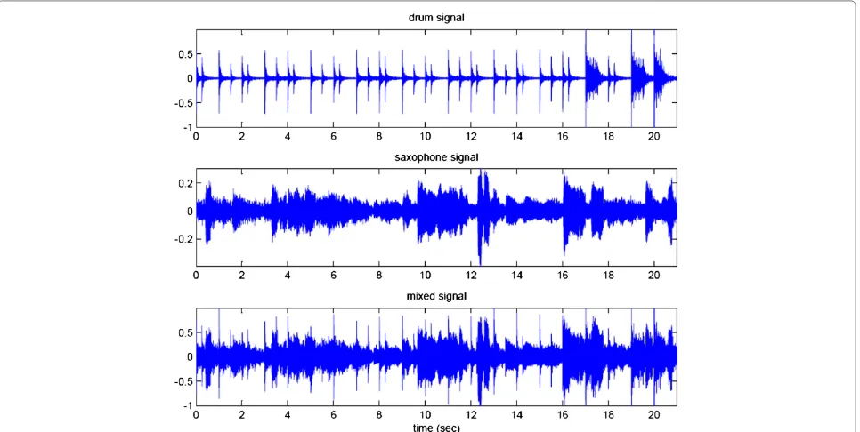
obtain a more robust performance in SIRs against differ-ent music source signals. Figure 7 shows the waveforms of a drum signal, a saxophone signal and the resulting mixed signal in “music 5”. Figure 8 displays the spectro-grams of these three signals. Figure 9 demonstrates the spectrograms of the reconstructed drum signal and sax-ophone signal using BGS-NMF-LSM. For the other five mixed signals, the performance of reconstructed signals in single-channel music source separation is shown at http://chien.cm.nctu.edu.tw/bgs-nmf.
5 Conclusions
This paper has presented the Bayesian group sparse learn-ing and applied it for slearn-ingle-channel nonnegative source separation. The basis vectors in NMF were grouped into
two partitions. The first group was the common bases which were used to explore the inter-segment repetitive characteristics, while the second was the individual bases which were applied to represent the intra-segment har-monic information. The LSM distribution was introduced to express sparse reconstruction weights for two groups of basis vectors. Bayesian learning was incorporated into group basis representation with model regularization. The MCMC algorithm or the Metropolis-Hastings algorithm was developed to conduct approximate inference of model parameters and hyperparameters. Model parameters were used to find the decomposed rhythmic signals and har-monic signals. Hyperparameters were used to control the sparsity of reconstructed weights and the generation of basis parameters. In the experiments, we implemented the
Figure 8Spectrograms of music 5 containing a drum signal, a saxophone signal, and their mixed signal.
proposed BGS-NMFs for underdetermined source sepa-ration. The convergence condition of sampling procedure for approximate inference was investigated. The perfor-mance of BGS-NMF-LP and BGS-NMF-LSM was shown to be robust to the different kinds of rhythmic and har-monic sources and mixing conditions. BGS-NMF-LSM outperformed the other NMFs in terms of SIRs. The BGS-NMF controlled by LSM distribution performed bet-ter than that controlled by Laplacian distribution. In the future, the system performance of BGS-NMF may be fur-ther improved by some ofur-ther considerations. For example, the numbers of common bases and individual bases could be automatically selected according to Bayesian frame-work by using marginal likelihood. The group sparse learning could be extended for constructing hierarchi-cal NMF where hierarchihierarchi-cal grouping of basis vectors is
examined. The underdetermined separation under dif-ferent number of sources and sensors could be tackled. Also, the online learning could be involved to update segment-based parameters and hyperparameters [33,34]. The evolutionary BGS-NMFs shall work for nonstation-ary single-channel blind source separation. In addition, more evaluations shall be conducted by using realistic data with larger amount of mixed speech signals from different application domains, such as meetings and call centers.
Appendix
Derivations for inference of BGS-NMF parameters and hyperparameters
We address some derivations for model inference of BGS-NMF parameters and hyperparameters. First, the
exponent of the likelihood functionp(XiT|[Ar(t+1)]i(1:j−1),
[A(t)r ]i(j+1:Dr),Sr(t),A(t)h ,S(t)h ,(t))in (16) is expressed by
− 1 2[(t)]
ii M
k=1
⎡ ⎣Xik−
j−1
m=1
[A(rt+1)]im[S(rt)]mk
−[Ar]ij[S(rt)]jk− Dr
m=j+1
[A(rt)]im[S(rt)]mk
− Dh
m=1
[A(ht)]im[S(ht)]mk
2
(26)
which can be manipulated as a quadratic function of parameter [Ar]ij and leads to (17). The
con-ditional posterior distribution p([Ar]ij|XiT, (t) Arij,
(t) Arij) is then derived by combining (17) and (11) and turns out to be
[Ar]
α(rjt)−1
ij
exp
⎧ ⎨ ⎩−
[Ar]2ij−2(μlikelA
rij −β
(t) rj [σAlikelrij ]
2)[Ar]
ij+[μlikelArij]2)
2[σAlikel
rij] 2
⎫ ⎬ ⎭
I[0,+∞[([Ar]ij)
(27)
which is proportional to (18). In addition, when finding the mode of (18), we take logarithm of (18) and solve a corresponding quadratic equation of [Ar]ijas
∂ ∂[Ar]ij
⎧ ⎨
⎩(α(t)rj −1)ln[Ar]ij−
([Ar]ij−μpostArij)2
2[σApost
rij ]
2
⎫ ⎬ ⎭=0
⇒[Ar]2ij−μ post
Arij[Ar]ij−(α
(t) rj −1)[σ
post Arij ]
2=0.
(28)
By defining =(μpostA
rij)
2+4(α(t)
rj −1)[σ post Arij ]
2, the mode
is determined by
μinstA
rij =
0, if<0
max{12(μpostA
rij + √
), 0}, else. (29)
On the other hand, following the model inference in Section 3.3, we continue to describe the MCMC sampling algorithm and the calculation of conditional posterior distributions for the remaining BGS-NMF hyperparame-ters{αr,βr,αh,βh,λr,λh,γr,δr,γh,δh}.
4. Sampling ofαrj.The hyperparameterα(trj+1)is sampled
according to a conditional posterior distribution which is
obtained by combining a likelihood function of [Ar]ijand
an exponential prior density of αrj with parameter λαrj. The resulting distribution is written by
p(αrj|[Ar(t+1)]ij,βrj(t))∝
1
(αrj)
exp{λpostαrj αrj}
Dr
I[0,+∞[(αrj)
(30)
where λpostαrj = lnβ
(t)
rj + (1/Dr)
Dr j=1ln[A
(t+1)
r ]ij−
(1/Dr)λαrj. This distribution does not belong to a known family, so the Metropolis-Hastings algorithm is applied. An instrumental distributionq(αrj)is obtained by fitting
the term within the brackets of (30) through a gamma distribution as detailed in [15].
5. Sampling ofβrj.The hyperparameterβrj(t+1) is
sam-pled according to a conditional posterior distribution which is obtained by combining a likelihood function of [Ar]ij and a gamma prior density ofβrj with parameters
{αβrj,ββrj}, i.e.,
p(βrj|[A(tr+1)]ij,αrj(t+1))∝(βrj)Drα (t+1)
rj
×exp ⎧ ⎨ ⎩−βrj
Dr
j=1
[A(tr+1)]ij ⎫ ⎬
⎭G(βrj|αβrj,ββrj). (31)
The resulting distribution is arranged as a new gamma distribution G(βrj|αpostβ
rj ,β
post
βrj ) where α
post βrj = 1 + Drα(trj+1) + αβrj and β
post βrj =
Dr j=1[A
(t+1)
r ]ij+ββrj. Here, we do not describe the sampling of α(thj+1) and
βhj(t+1) since the conditional posterior distributions for sampling these two hyperparameters are similar to those for sampling ofα(trj+1)andβrj(t+1).
6. Sampling of λrj or λhj. For sampling of scaling
parameterλ(trj+1), the conditional posterior distribution is obtained by
p(λrj|[Sr(t+1)]j(k=1:M),γrj(t),δrj(t))∝ M
k=1
p([Sr(t+1)]jk|λrj)p(λrj|γrj(t),δ(rjt))
∝(λrj)Mγ
(t)
rj exp
−Mλrj
δ(rjt)+ M
k=1
[Sr(t+1)]jk
.
(32)
7. Sampling of γrj. The sampling of LSM
likelihood function of λrj and an exponential prior
den-sity ofγrjwith parameterλγrj. The resulting distribution is expressed as
p(γrj|λrj(t+1),δrj(t))∝ 1 (γrj)
exp{λpostγrj γrj}I[0,+∞[(γrj),
(33)
where λpostγrj = lnδ
(t)
rj +
γrj−1 γrj lnλ
(t+1)
rj −λγrj. Again, we need to find an instrumental distribution q(γrj) which optimally fits the conditional posterior distribution p(γrj|λ(trj+1),δ(t)rj ). An approximate gamma distribution is found accordingly. The Metropolis-Hastings algorithm is then applied.
8. Sampling of δrj. The sampling of the other LSM parameter δ(trj+1) is performed by using the conditional posterior distribution which is derived from a likelihood function of λrj and a gamma prior density of δrj with parameters{αδrj,βδrj}
p(δrj|λ(trj+1),γ (t+1)
rj )∝(δrj)γ (t+1)
rj
exp{−δrjλ(trj+1)}G(δrj|αδrj,βδrj).
(34)
This distribution can be arranged as a new gamma distributionG(δrj|αδpost
rj ,β
post
δrj )whereα
post δrj = Drγ
(t+1)
rj +
αδrj andβ
post δrj = λ
(t+1)
rj +βδrj. Similarly, the conditional posterior distributions for sampling γhj(t+1) and δhj(t+1)
could be formulated by referring those for samplingγrj(t+1)
andδ(trj+1), respectively.
Competing interests
Both authors declare that they have no competing interests.
Acknowledgments
The authors acknowledge anonymous reviewers for their constructive feedback and helpful suggestions. This work has been partially supported by the National Science Council, Taiwan, Republic of China, under contract NSC 100-2628-E-009-028-MY3.
Received: 28 October 2012 Accepted: 13 May 2013 Published: 5 July 2013
References
1. A Cichocki, R Zdunek, S Amari, inProceedings of International Conference on Acoustic, Speech and Signal Processing (ICASSP). New algorithms for non-negative matrix factorization in applications to blind source separation (IEEE, Piscataway, 2006), pp. 621–624
2. PO Hoyer, Non-negative matrix factorization with sparseness constraints. J. Mach. Lear. Res.5, 1457–1469 (2004)
3. J-T Chien, H-L Hsieh, Convex divergence ICA for blind source separation. IEEE Trans. Audio, Speech, Language Process.20(1), 290–301 (2012) 4. R Kompass, A generalized divergence measure for nonnegative matrix
factorization. Neural Comput.19, 780–791 (2007)
5. H Lee, J Yoo, S Choi, Semi-supervised nonnegative matrix factorization. IEEE Signal Process. Lett.17(1), 4–7 (2010)
6. MD Plumbley, Algorithms for nonnegative independent component analysis. IEEE Trans. Neural Netw.14(3), 534–543 (2003)
7. CM Bishop,Pattern Recognition and Machine Learning(Springer Science, New York, 2006)
8. G Saon, J-T Chien, Bayesian sensing hidden Markov models. IEEE Trans. Audio, Speech Language, Process.20(1), 43–54 (2012)
9. ME Tipping, Sparse Bayesian learning and the relevance vector machine. J Mach. Learn. Res.1, 211–244 (2001)
10. SD Babacan, R Molina, AK Katsaggelos, Bayesian compressive sensing using Laplace priors. IEEE Trans. Image Process.19(1), 53–63 (2010) 11. H Lee, S Choi, inProceedings of the International Conference on Artificial
Intelligence and Statistics (AISTATS), vol. 15. Group nonnegative matrix factorization for EEG classification (JMLR, 2009), pp. 320–327 12. A Lefevre, F Bach, C Fevotte, Itakura-Saito, inProceedings of the
International Conference on Acoustic, Speech and Signal Processing (ICASSP). Nonnegative matrix factorization with group sparsity (Prague Congress Center, 22–27 May 2011), pp. 21–24
13. M Kim, J Yoo, K Kang, S Choi, inProceedings of the International Conference on Acoustic, Speech and Signal Processing (ICASSP). Blind rhythmic source separation: nonnegativity and repeatability (IEEE, Piscataway, 2010), pp. 2006–2009
14. AT, Cemgil, Bayesian inference for nonnegative matrix factorization models. University of Cambridge, Technical Report
CUED/F-INFENG/TR.609, 2008
15. S Moussaoui, D Brie, Mohammad-A Djafari, C Carteret, Separation of non-negative mixture of non-negative sources using a Bayesian approach and MCMC sampling. IEEE Trans. Signal Process.54(11), 4133–4145 (2006) 16. MN Schmidt, O Winther, LK Hansen, inProceedings of the International
Conference on Independent Component Analysis and Signal Separation, Paraty, March 2009. Lecture Notes in Computer Science, vol. 5441. Bayesian non-negative matrix factorization (Springer, Heidelberg, 2009), pp. 540–547
17. C Fevotte, SJ Godsill, A Bayesian approach for blind separation of sparse sources. IEEE Trans. Audio, Speech, Language Process.14(6), 2174–2188 (2006)
18. Z Duan, Y Zhang, C Zhang, Z Shi, Unsupervised single-channel music source separation by average harmonic structure modeling. IEEE Trans. on Audio, Speech, Language Process.16(4), 766–778 (2008) 19. MN Schmidt, RK Olsson, inProceedings of the Annual Conference of
International Speech Communication Association (INTERSPEECH) Single-channel speech separation using sparse non-negative matrix factorization (Pittsburgh, 17–21 September 2006), pp. 2614–2617 20. J-T Chien, H-L Hsieh, inProceedings of the Annual Conference of
International Speech Communication Association (INTERSPEECH). Bayesian group sparse learning for nonnegative matrix factorization (Portland, 9–13 September 2012), pp. 1552–1555
21. J Yoo, M Kim, K Kang, Choi S, inProceedings of the International Conference on Acoustic, Speech and Signal Processing (ICASSP)Nonnegative matrix partial co-factorization for drum source separation (IEEE, Piscataway, 2010), pp. 1942–1945
22. M Kim, J Yoo, K Kang, S Choi, Nonnegative matrix partial co-factorization for spectral and temporal drum source separation. IEEE J. Sel. Top. Signal Process.5(6), 1192-1204 (2011)
23. S Bengio, F Pereira, Y Singer, D Strelow, inAdvances in Neural Information Processing Systems (NIPS), vol. 22. Group sparse coding (NIPS La Jolla, 2009), pp. 82–89
24. R Jenatton, J Mairal, G Obozinski, F Bach, inProceedings of the International Conference on Machine Learning (ICML). Proximal methods for sparse hierarchical dictionary learning (Haifa, 21–25 June 2010)
25. PJ Garrigues, BA Olshausen, inAdvances in Neural Information Processing Systems (NIPS), vol. 23. Group sparse coding with a Laplacian scale mixture prior (NIPS La Jolla, 2010), pp. 676–684
26. R Salakhutdinov, A Mnih, inProceedings of the International Conference on Machine Learning (ICML). Bayesian probabilistic matrix factorization using Markov chain Monte Carlo (Helsinki, 5–9 July 2008), pp. 880–887 27. M Zhong, M Girolami, inProceedings of the International Conference on
Artificial Intelligence and Statistics (AISTATS). Reversible jump MCMC for non-negative matrix factorization (Clearwater Beach, 16–18 April 2009), pp. 663–670
29. M Marlin, BM, Schmidt, KP Murphy, inProceedings of the Conference on Uncertainty in Artificial Intelligence (UAI). Group sparse priors for covariance estimation ( Montreal, 18–21 June 2009), pp. 383–392
30. J-T Chien, C-C Chiang, inProceedings of the Annual Conference of International Speech Communication Association (INTERSPEECH). Group sparse hidden Markov models for speech recognition (Portland, 9–13 September 2012), pp. 2646–2649
31. J-T Chien, C-W Ting, Factor analyzed subspace modeling and selection. IEEE Trans. Audio, Speech Language Process.16(1), 239–248 (2008) 32. S Chib, E Greenberg, Understanding the Metropolis-Hastings algorithm.
Am. Statistician.49(4), 327–335 (1995)
33. J-T Chien, H.-L Hsieh, Nonstationary source separation using sequential and variational Bayesian learning. IEEE Trans. Neural Netw. Learn. Syst.
24(5), 681–694 (2013)
34. H-L Hsieh, J-T Chien, inProceedings of the International Conference on Acoustic, Speech and Signal Processing (ICASSP). Nonstationary and temporally-correlated source separation using Gaussian process (Prague Congress Center, 22–27 May 2011), pp. 2120–2123
doi:10.1186/1687-4722-2013-18
Cite this article as:Chien and Hsieh:Bayesian group sparse learning for
music source separation.EURASIP Journal on Audio, Speech, and Music Process-ing20132013:18.
Submit your manuscript to a
journal and benefi t from:
7Convenient online submission
7Rigorous peer review
7Immediate publication on acceptance
7Open access: articles freely available online
7High visibility within the fi eld
7Retaining the copyright to your article

![Figure 6 An estimated distribution of reconstruction weight ofcommon basis p([ Sr]jk |γrj, δrj).](https://thumb-us.123doks.com/thumbv2/123dok_us/9595968.1942044/10.595.56.290.516.700/figure-estimated-distribution-reconstruction-weight-ofcommon-basis-grj.webp)