R E S E A R C H
Open Access
Parallel computing subgradient method
for nonsmooth convex optimization over the
intersection of fixed point sets of
nonexpansive mappings
Hideaki Iiduka
**Correspondence: [email protected]
Department of Computer Science, Meiji University, 1-1-1 Higashimita, Tama-ku, Kawasaki-shi, Kanagawa, 214-8571, Japan
Abstract
Nonsmooth convex optimization problems are solved over fixed point sets of nonexpansive mappings by using a distributed optimization technique. This is done for a networked system with an operator, who manages the system, and a finite number of users, by solving the problem of minimizing the sum of the operator’s and users’ nondifferentiable, convex objective functions over the intersection of the operator’s and users’ convex constraint sets in a real Hilbert space. We assume that each of their constraint sets can be expressed as the fixed point set of an
implementable nonexpansive mapping. This setting allows us to discuss nonsmooth convex optimization problems in which the metric projection onto the constraint set cannot be calculated explicitly. We propose a parallel subgradient algorithm for solving the problem by using the operator’s attribution such that it can communicate with all users. The proposed algorithm does not use any proximity operators, in contrast to conventional parallel algorithms for nonsmooth convex optimization. We first study its convergence property for a constant step-size rule. The analysis
indicates that the proposed algorithm with a small constant step size approximates a solution to the problem. We next consider the case of a diminishing step-size sequence and prove that there exists a subsequence of the sequence generated by the algorithm which weakly converges to a solution to the problem. We also give numerical examples to support the convergence analyses.
MSC: 65K05; 90C25; 90C90
Keywords: fixed point; Krasnosel’ski˘ı-Mann algorithm; nonexpansive mapping; nonsmooth convex optimization; parallel algorithm; subgradient
1 Introduction
Convex optimization theory has been widely used to solve practical convex minimization problems over complicated constraints,e.g., convex optimization problems with afixed point constraint[–] and with avariational inequality constraint[–]. It enables us to consider constrained optimization problems in which the explicit form of the metric projection onto the constraint set is not always known;i.e., the constraint set is not simple in the sense that the projection cannot easily be computed (e.g., the constraint set is the
set of all minimizers of a convex function over a closed convex set [, ], or the set of zeros of a set-valued, monotone operator ([], Proposition .)).
This paper focuses on a networked system consisting of an operator, who manages the system, and a finite number of participating users, and it considers the problem of mini-mizing the sum of the operator’s and all users’nonsmooth convex functionsover the inter-section of the operator’s and all users’fixed point constraint setsin a real Hilbert space.
The motivations behind studying the problem are to devise optimization algorithms which have a wider range of application compared with the previous algorithms for smooth convex optimization (see,e.g., [, , , ]) and to tackle outstanding nonsmooth convex problems over complicated constraint sets (e.g., the minimal antenna-subset se-lection problem ([], Section .)).
Many algorithms have been presented for solving nonsmooth convex optimization. The Douglas-Rachford algorithm([], Chapters and ), [–],forward-backward algo-rithm([], Chapters and ), [, , ], andparallel proximal algorithm([], Propo-sition .), ([], Algorithm .), [] are useful to solve the sum of nonsmooth convex optimization problems over the whole space. They use theproximity operators([], Defi-nition .) of nonsmooth, convex functions. Theincremental subgradient method([], Section .) and theprojected multi-agent algorithms[–] can minimize the sum of nonsmooth, convex functions over a simple constraint set by using thesubgradients([], Section ) of the nonsmooth, convex functions instead of the proximity operators. To our knowledge, there are no references on parallel algorithms for nonsmooth convex op-timization with fixed point constraints.
In this paper, we propose aparallel subgradient algorithmfor nonsmooth convex op-timization with fixed point constraints. Our algorithm is founded on the ideas behind the two useful algorithms. The first is theKrasnosel’ski˘ı-Mann algorithm([], Subchap-ter .), [, ] for finding a fixed point of a nonexpansive mapping. It ensures that our algorithm converges to a point in the intersection of the fixed point sets of nonexpan-sive mappings. The second algorithm is theparallel proximal algorithm([], Proposi-tion .), ([], Algorithm .), [] for nonsmooth convex optimizaProposi-tion. Since the operator can communicate with all users, our parallel algorithm enables the operator to find a solution to the main problem by using information transmitted from all users.
This paper has three contributions in relation to other work on convex optimization. The first is that our algorithm does not use any proximity operators, in contrast to the algorithms presented in [, , –]. Our algorithm can use subgradients, which are well defined for any nonsmooth, convex functions.
The second contribution is that our parallel algorithm can be applied to nonsmooth convex optimization problems over the fixed point sets of nonexpansive mappings, while the previous algorithms work in nonsmooth convex optimization over simple constraint sets ([], Subchapter .), [, –] or smooth convex optimization over fixed point sets [–, , ].
This paper is organized as follows. Section gives the mathematical preliminaries and states the main problem. Section presents the parallel subgradient algorithm for solving the main problem and studies its convergence properties for a constant step size and a diminishing step size. Section provides numerical examples of the algorithm. Section concludes the paper.
2 Mathematical preliminaries
2.1 Nonexpansivity and subdifferentiability
LetHbe a real Hilbert space with inner product·,·and its induced norm · . LetN denote the set of all positive integers including zero.
A mapping, T: H→H, is said to benonexpansive([], Definition .(ii)) ifT(x) – T(y) ≤ x–y(x,y∈H).T is said to befirmly nonexpansive([], Definition .(i)) if
T(x) –T(y)+(Id –T)(x) – (Id –T)(y)≤ x–y(x,y∈H), where Id stands for the
identity mapping onH. It is clear that firm nonexpansivity implies nonexpansivity. The fixed point setofTis denoted byFix(T) :={x∈H: T(x) =x}. The metric projection ([], Subchapter ., Chapter ) onto a nonempty, closed convex setC(⊂H) is denoted byPC.
It is defined byPC(x)∈Candx–PC(x)=infy∈Cx–y(x∈H).
Proposition . Let T: H→H be nonexpansive,and let C(⊂H)be nonempty,closed, and convex.Then:
(i) ([],Corollary.)Fix(T)is closed and convex.
(ii) ([],Remark.(iii))(/)(Id +T)is firmly nonexpansive.
(iii) ([],Proposition.,equation(.))PCis firmly nonexpansive withFix(PC) =C.
Thesubdifferential([], Definition .), ([], Section ) off: H→Ris defined for allx∈Hby
∂f(x) :=u∈H:f(y)≥f(x) +y–x,u(y∈H).
We callu(∈∂f(x)) thesubgradientoff atx∈H.
Proposition .([], Proposition .(ii) and (iii)) Let f:H→Rbe continuous and convex withdom(f) :={x∈H: f(x) <∞}=H.Then∂f(x)=∅(x∈H).Moreover,for all x∈H,there existsδ> such that∂f(B(x;δ))is bounded,where B(x;δ)stands for a closed ball with center x and radiusδ.
2.2 Notation, assumptions, and main problem
This paper deals with a networked system with an operator (denoted by user ) andI users. Let
I:={, , . . . ,I} and I¯:={} ∪I.
We assume that useri(i∈ ¯I) has its own private mappings, denoted byf(i):H→Rand
T(i):H→H, and its own private nonempty, closed convex constraint set, denoted byC(i)
(⊂H). Moreover, we define
X:=
i∈ ¯I
FixT(i), f := i∈ ¯I
The following problem is discussed.
Problem . Assume that:
(A) T(i):H→H(i∈ ¯I) is firmly nonexpansive withFix(T(i)) =C(i). (A) f(i):H→R(i∈ ¯I) is continuous and convex withdom(f(i)) =H. (A) Useri(i∈ ¯I) can use its own privateT(i)and∂f(i).
(A) The operator can communicate with all users. (A) Xis nonempty.
The main objective is to findx∈X.
Assumption (A) and Proposition . ensure that ∂f(i)(x)=∅(i∈ ¯I,x∈H). Suppose
that the operator setsxˆ∈H. Accordingly, (A) guarantees that the operator can trans-mitxˆ to all users. Assumption (A) implies that useri(i∈ ¯I) can computein parallel
ˆ
x(i):=xˆ(i)(x,ˆ T(i),∂f(i)) by using the informationxˆ transmitted from the operator and its
own private information. Moreover, (A) ensures that the operator has access to allxˆ(i)
and can computex¯:=x(¯xˆ(),xˆ(), . . . ,xˆ(I)). The next section describes a sufficient condition
for satisfying (A).
3 Parallel subgradient algorithm for nonsmooth convex optimization over fixed point sets
This section presents a parallel subgradient algorithm for solving Problem ..
Algorithm .
Step . The operator (user) and all users setα(∈(, )) and(λn)n∈N(⊂(,∞)). The op-erator choosesx∈Harbitrarily and transmits it to all users.
Step . Givenxn∈H, useri(i∈ ¯I) computesx(ni)∈Hby
⎧ ⎨ ⎩
gn(i)∈∂f(i)(xn),
x(ni):=αxn+ ( –α)T(i)(xn–λngn(i)).
Useri(i∈I) transmitsx(ni)to the operator. Step . The operator computesxn+∈Has
xn+:=
I+
i∈ ¯I
x(ni)
and transmits it to all users. Putn:=n+ , and go to Step .
Our convergence results depend on the following assumption.
Assumption . The sequence, (x(ni))n∈N(i∈ ¯I), generated by Algorithm . is bounded.
We shall provide examples satisfying Assumption .. Useri(i∈ ¯I) in an actual network [, –] has a boundedC(i)defined by the intersection of simple, closed convex setsC(i) k
(k∈K(i):={, , . . . ,K(i)}) (e.g.,C(i)
k is an affine subspace, a half-space, or a hyperslab) and
P(ki):=PC(i)
k
can easily be computed within a finite number of arithmetic operations [],
is easily computed (e.g.,X(i)=Fix(P(i)) is a closed ball with a large enough radius). Since
X(i)is bounded andX⊂C(i)⊂X(i) (i∈ ¯I),Xis also bounded. Hence, the continuity and convexity off ensure thatX=∅,i.e., (A) holds ([], Proposition .). In this case, user
ican use
T(i):=
Id +
k∈K(i) P(ki)
with FixT(i)=C(i)⊂X(i). ()
Proposition .(ii) and (iii) guarantee thatT(i)defined by () satisfies the firm
nonexpan-sivity condition. Moreover, userican compute
x(ni):=P(i)αxn+ ( –α)T(i)
xn–λngn(i)
()
instead of x(ni) in Algorithm .. Since X(i) is bounded and (x(ni))n∈N ⊂X(i), (xn(i))n∈N is
bounded. We can prove that Algorithm . with () satisfies the properties in the main theorems (Theorems . and .) by referring to the proofs of the theorems.
The following lemma yields some properties of Algorithm . that will be used to prove the main theorems.
Lemma . Suppose that Assumptions(A)-(A)and.are satisfied,lim supn→∞λn<∞,
and y(ni):=T(i)(xn–λngn(i)) (n∈N,i∈ ¯I).Then the following properties hold: (i) (gn(i))n∈N,(y(ni))n∈N(i∈ ¯I),and(xn)n∈Nare bounded.
(ii) For allx∈Xand for alln∈N,
xn+–x≤ xn–x+Mλn–
–α I+
i∈ ¯I
xn–y(ni)
,
whereM:=maxi∈ ¯I(sup{|y (i)
n –x,gn(i)|:n∈N}) <∞. (iii) For allx∈Xand for alln∈N,
xn+–x≤ xn–x+
( –α)λn
I+
f(x) –f(xn)
+M( –α)λn,
whereM:=maxi∈ ¯I(sup{gn(i):n∈N}) <∞.
Proof (i) Assumption . and the definition ofxn (n∈N) ensure the boundedness of
(xn)n∈N. Hence, from (A) and Proposition ., we find that (gn(i))n∈N(i∈ ¯I) is also bounded.
Assumption (A) implies that, for allx∈X, for alln∈N, and for alli∈ ¯I, y(ni)–x=T(i)xn–λngn(i)
–T(i)(x)≤xn–λngn(i)
–x.
Accordingly, the boundedness of (xn)n∈Nand (gn(i))n∈N(i∈ ¯I) andlim supn→∞λn<∞imply
that (y(ni))n∈N(i∈ ¯I) is also bounded.
(ii) Choose x ∈ X arbitrarily and put M := maxi∈ ¯I(sup{|y (i)
n –x,gn(i)|: n ∈ N}).
Lemma .(i) guarantees thatM<∞. Assumption (A) ensures that, for alln∈Nand
for alli∈ ¯I,
y(ni)–x=T(i)xn–λngn(i)
–T(i)(x)
≤xn–λngn(i)
–x–xn–λngn(i)
which, together withx–y=x– x,y+y(x,y∈H), means that
y(ni)–x≤ xn–x– λn
xn–x,gn(i)
+λngn(i)
–xn–y(ni)
+ λn
xn–y(ni),gn(i)
–λngn(i)
≤ xn–x–xn–y(ni)
+Mλn. ()
The convexity of · implies that, for alln∈Nand for alli∈ ¯I, x(ni)–x=α(xn–x) + ( –α)
y(ni)–x
≤αxn–x+ ( –α)y(ni)–x
, ()
which, together with (), means that, for alln∈Nand for alli∈ ¯I, x(ni)–x≤ xn–x– ( –α)xn–y(ni)
+Mλn.
Summing up this inequality over alliguarantees that, for alln∈N,
I+
i∈ ¯I
x(ni)–x≤ xn–x–
–α I+
i∈ ¯I
xn–y(ni)
+Mλn.
Accordingly, from the definition ofxn(n∈N) and the convexity of · , we find that, for
alln∈N,
xn+–x≤
I+
i∈ ¯I
x(ni)–x
≤ xn–x–
–α I+
i∈ ¯I
xn–y(ni)
+Mλn.
(iii) Choosex∈Xarbitrarily. Then () and the definition ofgn(i)(n∈N,i∈ ¯I) imply that,
for alln∈Nand for alli∈ ¯I, y(ni)–x≤ xn–x+ λn
x–xn,gn(i)
+λng(ni)
≤ xn–x+ λn
f(i)(x) –f(i)(xn)
+Mλn,
whereM:=maxi∈ ¯I(sup{gn(i): n∈N}) <∞(M<∞is guaranteed by Lemma .(i)).
Accordingly, () guarantees that, for alln∈Nand for alli∈ ¯I, x(ni)–x≤ xn–x+ ( –α)λn
f(i)(x) –f(i)(xn)
+M( –α)λn,
which, together with the convexity of · andf :=
i∈ ¯If(i), implies that, for alln∈N,
xn+–x≤
I+
i∈ ¯I
x(ni)–x
≤ xn–x+
( –α)λn
I+
i∈ ¯I
f(i)(x) –f(i)(x n)
+M( –α)λn
=xn–x+
( –α)λn
I+
f(x) –f(xn)
+M( –α)λn.
This completes the proof.
3.1 Constant step-size rule
The discussion in this subsection makes the following assumption.
Assumption . Useri(i∈ ¯I) has (λn)n∈Nsatisfying
(C) λn:=λ∈(,∞) (n∈N).
Let us perform a convergence analysis on Algorithm . under Assumption ..
Theorem . Suppose that Assumptions(A)-(A), .,and.hold.Then the sequence, (xn)n∈N,generated by Algorithm.satisfies,for all i∈ ¯I,
lim inf
n→∞xn–T (i)(x
n)
≤Mλ and lim inf
n→∞ f(xn)≤f
+(I+ )Mλ
,
where Mand Mare constants defined as in Lemma.,M:=maxi∈ ¯I(sup{xn–y(ni): n∈ N}),and M:= (I+ )M/( –α) + M
√
M+Mλ.
Let us compare Algorithm . under the assumptions in Theorem . with previous algo-rithms ([], Section .), ([], Chapters and ), [, –]. The following sequence (xn)n∈N is generated by a parallel proximal algorithm ([], Chapters and ), [, ,
] that can be applied to signal and image processing: given (λn)n∈N ⊂(, ),y(ni)∈H,
(a(ni))n∈N⊂H(i= , , . . . ,m), andxn∈H,
⎧ ⎪ ⎪ ⎪ ⎪ ⎪ ⎨ ⎪ ⎪ ⎪ ⎪ ⎪ ⎩
p(ni):=proxγf(i)/ω(i)y(ni)+a(ni) (i= , , . . . ,m), pn:=
m
i=ω(i)p (i) n,
y(ni+) :=y(ni)+λn(pn–xn–p(ni)) (i= , , . . . ,m),
xn+:=xn+λn(pn–xn),
()
whereγ∈(, ), (ω(i))m
i=(⊂(, )) satisfies
m
i=ω(i)= , andproxf(i)stands for the proxim-ity operatoroff(i)which maps everyx∈Hto the unique minimizer off(i)+ (/)x–·.
(See ([], Tables . and .) for examples of convex functions for which proximity operators can be explicitly computed.) When (λn)n∈Nsatisfiesn∞=λn( –λn) =∞(e.g.,
λn:=λ∈(, ) (n∈N) satisfies this condition) and
∞
n=λna (i)
n<∞(i= , , . . . ,m),
(xn)n∈Nin algorithm () converges to a minimizer of
m
i=f(i)overH([], Theorem .).
Suppose thatC(i) (i∈ ¯I) is simple in the sense thatP
C(i) can easily be computed (e.g., C(i)is an affine subspace, a half-space, or a hyperslab). Algorithm . withλn:=λ∈(,∞)
(n∈N) andT(i)=PC(i)(i∈ ¯I) is as follows: givengn(i)∈∂f(i)(xn) (i∈ ¯I),
⎧ ⎨ ⎩
x(ni):=αxn+ ( –α)PC(i)(xn–λgn(i)) (i= , , . . . ,I),
xn+:=I+
i∈ ¯Ix (i) n.
We can see that algorithm () uses the subgradientgn(i)∈∂f(i)(xn), while algorithm () uses
the proximity operator off(i). Theorem . says that under the assumptions in Theorem .
algorithm () satisfies, for alli∈ ¯I,
lim inf
n→∞xn–PC(i)(xn)
≤Mλ and lim inf
n→∞ f(xn)≤f
+(I+ )Mλ
.
Therefore, we can expect that algorithm () with a small enoughλapproximates a mini-mizer off overi∈ ¯IC(i).
Let us also assumeC:=C(i)(i∈ ¯I). The followingincremental subgradient method([],
Section .) can solve the problem of minimizingf overC: givenλ> andxn=x()n =
x(nI–) ∈RN,
⎧ ⎨ ⎩
xn(i):=PC(xn(i–)–λgn(i)), gn(i)∈∂f(i)(x(ni–)) (i= , , . . . ,I),
xn+:=x(nI).
()
Algorithm () satisfies
lim inf
n→∞ f(xn)≤f
∗+Dλ
,
where{x∈C:f(x) =f∗:=infy∈Cf(y)} =∅,D:=
i∈ID(i),D(i):=sup{g: g∈∂f(i)(xn)∪
∂f(i)(x(i–)
n ),n∈N}(i∈I), and one assumes thatD(i)<∞(i∈I) ([], Proposition ..).
In contrast to the above convergence analysis of the incremental subgradient method (), Theorem . guarantees that, ifx∈C, the parallel algorithm () withPC=PC(i) (i∈ ¯I) satisfies
xn∈C (n∈N) and lim inf
n→∞ f(xn)≤f
∗+(I+ )Mλ
.
We can see that the previous algorithms () and () can be applied to the case where the projections onto constraint sets can easily be computed, whereas Algorithm . can be applied even whenC(i)(i∈ ¯I) has a more complicated form (see,e.g., ()).
Now, we shall prove Theorem ..
Proof First, let us show that
lim inf
n→∞
i∈ ¯I
xn–y(ni)
≤(I+ )Mλ
–α . ()
Assume that () does not hold. Accordingly, we can chooseδ> such that
lim inf
n→∞
i∈ ¯I
xn–y(ni)
>(I+ )Mλ
–α + δ.
The property of the limit inferior of (i∈ ¯Ixn–yn(i))n∈Nguarantees that there existsn∈ Nsuch thatlim infn→∞i∈ ¯Ixn–y(ni)–δ≤
for alln≥n,
i∈ ¯I
xn–y(ni)
>(I+ )Mλ
–α +δ.
Hence, Lemma .(ii) leads us to that, for alln≥nand for allx∈X,
xn+–x<xn–x+Mλ–
–α I+
(I+ )Mλ
–α +δ
=xn–x–
–α I+ δ.
Therefore, induction ensures that, for alln≥nand for allx∈X,
≤ xn+–x<xn–x
– –α
I+ δ(n+ –n).
Since the right side of the above inequality approaches minus infinity when n
di-verges, we have a contradiction. Therefore, () holds. Since lim infn→∞xn–y(ni) ≤
lim infn→∞i∈ ¯Ixn–y(ni)(i∈ ¯I), we also find that
lim inf
n→∞xn–y
(i) n
≤(I+ )Mλ
–α (i∈ ¯I). ()
From the triangle inequality we see that, for alln∈Nand for alli∈ ¯I,xn–T(i)(xn) ≤ xn–y(ni)+yn(i)–T(i)(xn), which, together withM:=maxi∈ ¯I(sup{xn–y(ni): n∈N}) <∞
andy(ni)–T(i)(xn) ≤ (xn–λgn(i)) –xn ≤√Mλ(n∈N,i∈ ¯I), means that, for alln∈N
and for alli∈ ¯I,
xn–T(i)(xn)
≤xn–y(ni)
+ MMλ+Mλ.
Thus, () guarantees that
lim inf
n→∞xn–T
(i)(x n)
≤lim inf
n→∞xn–y
(i) n
+ (MM+Mλ)λ
=lim inf
n→∞xn–y
(i) n
+ (MM+Mλ)λ
≤
(I+ )M
–α +
MM+Mλ
λ.
Next, let us show that
lim inf
n→∞ f(xn)≤f
+(I+ )Mλ
. ()
Assume that () does not hold. Since (A) guarantees thatx∈Xexists such thatf(x) =
f, we can choose > such that
lim inf
n→∞ f(xn) >f
x+(I+ )Mλ
From the property of the limit inferior of (f(xn))n∈N, there exists n ∈ N such that
lim infn→∞f(xn) – ≤f(xn) for alln≥n. Accordingly, for alln≥n,
f(xn) –f
x>(I+ )Mλ
+ . ()
Therefore, from Lemma .(iii) and () we see that, for alln≥n,
xn+–x
<xn–x
+M( –α)λ+
( –α)λ I+
–(I+ )Mλ
–
=xn–x
–( –α)λ I+ ,
which implies that, for alln≥n,
xn+–x
<xn–x
–( –α)λ
I+ (n+ –n).
Since the above inequality does not hold for large enoughn, we have arrived at a
contra-diction. Therefore, () holds. This completes the proof.
3.2 Diminishing step-size rule
The discussion in this subsection makes the following assumption.
Assumption . Useri(i∈ ¯I) has (λn)n∈Nsatisfying
(C) lim
n→∞λn= and ∞
n=
λn=∞.
An example of (λn)n∈Nisλn:= /(n+ )a(n∈N), wherea∈(, ].
Let us perform a convergence analysis on Algorithm . under Assumption ..
Theorem . Suppose that Assumptions(A)-(A), .,and.hold.Then there exists a subsequence of(xn)n∈Ngenerated by Algorithm.which weakly converges to a point in X.
Let us compare Algorithm . under the assumptions in Theorem . with the previous gradient algorithms with diminishing step sizes ([], Section .), []. Suppose thatC:= C(i) (i∈ ¯I). The sequence (x
n)n∈N is generated by the incremental subgradient method
([], Section .) as follows (see also ()): given (λn)n∈Nwith (C), andxn=x()n =x(nI–) ∈ RN,
⎧ ⎨ ⎩
x(ni):=PC(x(ni–)–λngn(i)), gn(i)∈∂f(i)(x(ni–)) (i= , , . . . ,I),
xn+:=x(nI).
The incremental subgradient method satisfies
lim inf
n→∞ f(xn) =f
∗,
where{x∈C: f(x) =f∗:=infy∈Cf(y)} =∅,D(i):=sup{g: g∈∂f(i)(xn)∪∂f(i)(x(ni–)),n∈N}
The following broadcast gradient method ([], Algorithm .) can minimize the sum of convex, smooth functionals over the intersection of fixed point sets: givenx(i)∈H(i∈ ¯I),
⎧ ⎨ ⎩
x(ni)+:=αnx(i)+ ( –αn)T(i)(xn–λn∇f(i)(xn)) (i= , , . . . ,I),
xn+:=I+ i∈ ¯Ix(ni+) ,
where∇f(i)(i∈I) is the Lipschitz continuous gradient off(i), and (α
n)n∈Nand (λn)n∈Nare
slowly diminishing sequences such asλn:= /(n+ )aandαn:= /(n+ )b (n∈N), where
a∈(, /),b∈(a, –a). The sequence (xn)n∈Nweakly converges to a minimizer off over
X([], Theorem .).
Meanwhile, Algorithm . works even whenf(i)(i∈I) is convex and nondifferentiable
andT(i)(i∈ ¯I) is firmly nonexpansive. Theorem . guarantees that there exists a sub-sequence of (xn)n∈Nin Algorithm . with (C) such that it weakly converges to a point
inX.
The rest of this subsection gives the proof of Theorem ..
Proof Fixx∈Xarbitrarily. We will distinguish two cases.
Case : Suppose that m∈Nexists such that xn+–x ≤ xn–x (n≥m).
Lem-ma .(ii) means that, for alln∈N,
–α I+
i∈ ¯I
xn–y(ni)≤ xn–x–xn+–x+Mλn,
which, together with the existence oflimn→∞xn–xandlimn→∞λn= , implies that
limn→∞( –α)/(I+ )i∈ ¯Ixn–y(ni)= ,i.e.,
lim
n→∞xn–y
(i)
n= (i∈ ¯I). ()
Moreover, (A) (the nonexpansivity ofT(i)(i∈ ¯I)) guarantees that, for alln∈Nandi∈ ¯I, y(ni)–T(i)(xn) ≤ (xn–λngn(i)) –xn ≤
√
Mλn, which, together withlimn→∞λn= , means
that
lim
n→∞y
(i)
n –T(i)(xn)= (i∈ ¯I). ()
Since the triangle inequality impliesxn–T(i)(xn) ≤ xn–y(ni)+y(ni)–T(i)(xn)(n∈N,
i∈ ¯I), () and () guarantee that
lim
n→∞xn–T
(i)(x
n)= (i∈ ¯I). ()
Here, we define, for alln∈N,
Mn:= ( –α)
I+
f(xn) –f(x)
–Mλn
.
Then Lemma .(iii) implies that, for alln∈N,λnMn≤ xn+–x–xn–x, which
that
∞
n=
λnMn<∞.
Therefore, from∞n=λn=∞, we find that
lim inf
n→∞ Mn≤. ()
Indeed, let us assume thatlim infn→∞Mn≤ does not hold,i.e.,lim infn→∞Mn> . Then
there existm∈Nandγ > such thatMn≥γ for alln≥m. From
∞
n=λn=∞, we
have∞=γ∞n=m λn≤
∞
n=mλnMn<∞, which is a contradiction. Hence, () holds. Accordingly, fromlimn→∞λn= , we find that
≥lim inf
n→∞
I+
f(xn) –f(x)
–Mλn
=
I+ lim infn→∞
f(xn) –f(x)
–M lim n→∞λn
=
I+ lim infn→∞
f(xn) –f(x)
.
This means there is a subsequence (xnl)l∈Nof (xn)n∈Nsuch that
lim
l→∞f(xnl) =lim infn→∞ f(xn)≤f(x) (x∈X). ()
The boundedness of (xnl)l∈N guarantees that (xnlm)m∈N (⊂(xnl)l∈N) exists such that (xnlm)m∈N weakly converges tox∈H. Here, fixi∈ ¯I arbitrarily and assume thatx∈/
Fix(T(i)). From Opial’s condition ([], Lemma ), (), and the nonexpansivity ofT(i), we
produce a contradiction:
lim inf
m→∞xnlm–x<lim infm→∞xnlm–T (i)(x
)
=lim inf
m→∞xnlm–T (i)(x
nlm) +T(i)(xnlm) –T(i)(x)
=lim inf
m→∞T
(i)(x
nlm) –T(i)(x)
≤lim inf
m→∞ xnlm–x.
Hence,x∈Fix(T(i)) (i∈ ¯I),i.e.,x∈X. Moreover, sincef is weakly lower semicontinuous
([], Theorem .) and (), we find that
f(x)≤lim inf
m→∞f(xnlm) =llim→∞f(xnl)≤f(x) (x∈X). Therefore,x∈X.
Let us take another subsequence (xnlk)k∈N (⊂ (xnl)l∈N) which weakly converges to x∈H. A similar discussion to the one for obtainingx∈Xensures thatx∈X.
Lemma ) imply that
lim
n→∞xn–x=mlim→∞xnlm–x<mlim→∞xnlm–x
= lim
n→∞xn–x=klim→∞xnlk–x<klim→∞xnlk –x
= lim
n→∞xn–x,
which is a contradiction. Hence,x=x. Accordingly, any subsequence of (xnl)l∈N con-verges weakly tox∈X,i.e., (xnl)l∈N converges weakly tox∈X
. This means thatx is
a weak cluster point of (xn)n∈Nand belongs toX. A similar discussion to the one for
ob-tainingx=xguarantees that there is only one weak cluster point of (xn)n∈N, and hence,
we can conclude that, in Case , (xn)n∈Nweakly converges to a point inX.
Case : Suppose that (xnj) (⊂(xn)n∈N) exists such thatxnj–x<xnj+–xfor allj∈N. Lemma .(ii) means that, for allj∈N,
–α I+
i∈ ¯I
xnj–y
(i) nj
≤ xnj–x
–x nj+–x
+M
λnj<Mλnj,
which, together withlimn→∞λn= , implies that
lim
j→∞xnj–y
(i)
nj= (i∈ ¯I). ()
Therefore, a similar discussion to the one for obtaining () ensures that
lim
j→∞
xnj–T
(i)(x
nj)= (i∈ ¯I). ()
Since Lemma .(iii) implies thatλnjMnj≤ xnj–x–xnj+–x< (j∈N) andλnj> (j∈N), we find thatMnj< (j∈N),i.e., for allj∈N,
I+
f(xnj) –f(x)
<Mλnj.
Sincelimn→∞λn= implies that
I+ lim supj→∞
f(xnj) –f(x)
≤M lim j→∞λnj= ,
we find that
lim sup
j→∞ f(xnj)≤f(x) (x∈X). ()
Inequality () ensures the existence of (xnjk)k∈Nof (xnj)j∈Nsuch that
lim
k→∞f(xnjk) =lim supj→∞ f(xnj)≤f(x) (x∈X). () Since (xnjk)k∈Nis bounded, we have (xnjk
lower semicontinuity off ([], Theorem .) and () guarantee that
f(x∗)≤lim inf
l→∞ f(xnjkl) =klim→∞f(xnjk)≤f(x) (x∈X),i.e.,x∗∈X
.
Therefore, there exists a subsequence of (xn)n∈Nsuch that it weakly converges to a point
inX. This completes the proof.
4 Numerical examples
Let us look at some numerical examples to see how Algorithm . works depending on the choice of step size. Consider the following problem: givena(i)> ,b(i)∈R,d(i)
k ∈R, and
c(ki)∈RI+withc(i)
k = (i∈ ¯I:={, , , . . . ,I},k∈K:={, , . . . ,K}),
minimize
i∈ ¯I
a(i)x(i)+b(i) subject to (x(i))i∈ ¯I∈C∩
i∈ ¯I
C(i), ()
wheref(i)(x) :=|a(i)x+b(i)|(i∈ ¯I,x∈R),C(i)
k (⊂RI+) (i∈ ¯I,k∈K) is a half-space defined
byCk(i):={x∈RI+: c(i) k,x ≤d
(i) k },C(i):=
k∈KCk(i)=∅(i∈ ¯I),C(⊂RI+) is a closed ball,
andC∩i∈ ¯IC(i)=∅.
We will assume that useri(i∈ ¯I) computes
x(ni):=PC
αxn+ ( –α)T(i)
xn–λngn(i)
(n∈N),
whereT(i)is defined by
T(i):=
Id +PC
k∈K
P(ki)
,
P(ki):=P
C(ki)(k∈K),g (i)
n = (, , . . . , ,g¯(ni), , , . . . , ), and
¯
gn(i)∈∂f(i)(xn(i)) :=
⎧ ⎪ ⎪ ⎨ ⎪ ⎪ ⎩
–a(i) (–∞<x n(i)< –b
(i)
a(i)), [–a(i),a(i)] (xn(i)= –b
(i)
a(i)), a(i) (–b(i)
a(i) <xn(i)<∞).
Since (x(ni))n∈N⊂C(i∈ ¯I), the boundedness ofCmeans Assumption . holds (see also
() and ()). Moreover, the continuity and convexity off ensures thatX=∅([],
Propo-sition .). The projectionsPC andPk(i)(i∈ ¯I,k∈K) can be computed within a finite
number of arithmetic operations ([], Chapter ), and hence,T(i) (i∈ ¯I) can also be
computed easily. Userican randomly choosea¯(i)∈∂f(i)(–b(i)/a(i)) = [–a(i),a(i)].
The experiment used a .-inch MacBook Pro with a . GHz Intel Core i processor and GB MHz DDR memory. Algorithm . was written in MATLAB .. We set I:= andK:= , and useda(i),b(i),ck(i),dk(i), anda¯(i)randomly generated by MATLAB. We used
α:=
, λn:=
,
,
(n+ )a (n∈N), wherea= ., .
We used the following performance measures: for eachn∈N,
Dn:=
s=
i∈ ¯I
xn(s) –T(i)
xn(s)
and
Fn:=
s=
i∈ ¯I
a(i)xn(i)(s) +b(i),
where (xn(s))n∈N is the sequence generated by the initial point x(s) (s= , , . . . , )
and Algorithm ., and xn(s) := (xn(i)(s))i∈ ¯I (n∈N, s= , , . . . , ).Dn (n∈N) stands
for the mean value of the sums of the squared distances between xn(s) and T(i)(xn(s))
(i∈ ¯I, s= , , . . . , ). If (Dn)n∈N converges to , Algorithm . converges to a point
ini∈ ¯IFix(T(i)) =C∩
i∈ ¯IC(i).Fn(n∈N) is the mean value of the objective function
i∈ ¯If(i)(xn(i)(s)) (s= , , . . . , ).
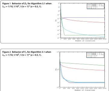
Figure indicates the behavior ofDnfor Algorithm .. We can see that the sequences
generated by Algorithm . withλn:= /(n+ )a (a= ., ,n∈N) converge to a point
ini∈ ¯IFix(T(i)). Meanwhile, Figure shows that Algorithm . withλ
n:= / (n∈N)
does not converge ini∈ ¯IFix(T(i)), and (D
n)n∈Nin Algorithm . withλn:= /(n∈N)
initially decreases. This is because the use ofλ:= /satisfieslim inf
n→∞xn–T(i)(xn) ≤
M/≈ (i∈ ¯I) (see Theorem .).
Figure plots the behavior ofFnfor Algorithm . and shows that Algorithm . with
λn:= /(n+ ) (n∈N) is stable during the early iterations and converges to a solution to
problem (), as promised by Theorem .. This figure indicates that the (Fn)n∈Ngenerated
Figure 1 Behavior ofDnfor Algorithm 3.1 when λn:= 1/10, 1/103, 1/(n+ 1)a(a= 0.5, 1).
by Algorithm . withλ:= /(n∈N) decreases slowly. Therefore, Figures and , and
Theorem . show that Algorithm . withλn:= /(n+ ) (n∈N) converges to a solution
to problem ().
5 Conclusion
This paper discussed the problem of minimizing the sum of nondifferentiable, convex functions over the intersection of the fixed point sets of firmly nonexpansive mappings in a real Hilbert space. It presented a parallel algorithm for solving the problem. The parallel algorithm does not use any proximity operators, in contrast to conventional parallel al-gorithms. Moreover, the parallel algorithm can work in nonsmooth convex optimization over constraint sets onto which projections cannot be always implemented, while the con-ventional incremental subgradient method can only be applied when the constraint set is simple in the sense that the projection onto it can easily be implemented. We studied its convergence properties for the two step-size rules, a constant step size and a diminishing step size. We showed that the algorithm with a small constant step size will approximate a solution to the problem, while there exists a subsequence of the sequence generated by the algorithm with a diminishing step size which weakly converges to a solution to the problem. We also gave numerical examples to support the convergence analyses.
Competing interests
The author declares that they have no competing interests.
Acknowledgements
I am sincerely grateful to the associate editor Lai-Jiu Lin and the two anonymous reviewers for helping me improve the original manuscript. This work was supported by the Japan Society for the Promotion of Science through a Grant-in-Aid for Scientific Research (C) (15K04763).
Received: 10 October 2014 Accepted: 1 May 2015
References
1. Combettes, PL: A block-iterative surrogate constraint splitting method for quadratic signal recovery. IEEE Trans. Signal Process.51(7), 1771-1782 (2003)
2. Iiduka, H: Fixed point optimization algorithms for distributed optimization in networked systems. SIAM J. Optim.23, 1-26 (2013)
3. Iiduka, H: Acceleration method for convex optimization over the fixed point set of a nonexpansive mapping. Math. Program.149, 131-165 (2015)
4. Iiduka, H, Hishinuma, K: Acceleration method combining broadcast and incremental distributed optimization algorithms. SIAM J. Optim.24, 1840-1863 (2014)
5. Iiduka, H, Yamada, I: A use of conjugate gradient direction for the convex optimization problem over the fixed point set of a nonexpansive mapping. SIAM J. Optim.19(4), 1881-1893 (2009)
6. Maingé, PE: A viscosity method with no spectral radius requirements for the split common fixed point problem. Eur. J. Oper. Res.235, 17-27 (2014)
7. Yamada, I: The hybrid steepest descent method for the variational inequality problem over the intersection of fixed point sets of nonexpansive mappings. In: Butnariu, D, Censor, Y, Reich, S (eds.) Inherently Parallel Algorithms for Feasibility and Optimization and Their Applications, pp. 473-504. Elsevier, Amsterdam (2001)
8. Yao, Y, Cho, YJ, Liou, YC: Algorithms of common solutions for variational inclusions, mixed equilibrium problems and fixed point problems. Eur. J. Oper. Res.212, 242-250 (2011)
9. Facchinei, F, Pang, J, Scutari, G, Lampariello, L: VI-constrained hemivariational inequalities: distributed algorithms and power control in ad-hoc networks. Math. Program.145, 59-96 (2014)
10. Iiduka, H: Iterative algorithm for solving triple-hierarchical constrained optimization problem. J. Optim. Theory Appl.
148, 580-592 (2011)
11. Iiduka, H: Iterative algorithm for triple-hierarchical constrained nonconvex optimization problem and its application to network bandwidth allocation. SIAM J. Optim.22(3), 862-878 (2012)
12. Iiduka, H, Yamada, I: Computational method for solving a stochastic linear-quadratic control problem given an unsolvable stochastic algebraic Riccati equation. SIAM J. Control Optim.50, 2173-2192 (2012)
13. Maingé, PE: Projected subgradient techniques and viscosity methods for optimization with variational inequality constraints. Eur. J. Oper. Res.205, 501-506 (2010)
14. Combettes, PL, Bondon, P: Hard-constrained inconsistent signal feasibility problems. IEEE Trans. Signal Process.47(9), 2460-2468 (1999)
16. Yamada, I, Yukawa, M, Yamagishi, M: Minimizing the Moreau envelope of nonsmooth convex functions over the fixed point set of certain quasi-nonexpansive mappings. In: Bauschke, HH, Burachik, RS, Combettes, PL, Elser, V, Luke, DR, Wolkowicz, H (eds.) Fixed-Point Algorithms for Inverse Problems in Science and Engineering, pp. 345-390. Springer, Berlin (2011)
17. Combettes, PL, Pesquet, JC: A Douglas-Rachford splitting approach to nonsmooth convex variational signal recovery. IEEE J. Sel. Top. Signal Process.1, 564-574 (2007)
18. Combettes, PL, Pesquet, JC: Proximal splitting methods in signal processing. In: Bauschke, HH, Burachik, RS, Combettes, PL, Elser, V, Luke, DR, Wolkowicz, H (eds.) Fixed-Point Algorithms for Inverse Problems in Science and Engineering, pp. 185-212. Springer, Berlin (2011)
19. Eckstein, J, Bertsekas, DP: On the Douglas-Rachfold splitting method and proximal point algorithm for maximal monotone operators. Math. Program.55, 293-318 (1992)
20. Lions, PL, Mercier, B: Splitting algorithms for the sum of two nonlinear operators. SIAM J. Numer. Anal.16, 964-979 (1979)
21. Combettes, PL: Iterative construction of the resolvent of a sum of maximal monotone operators. J. Convex Anal.16, 727-748 (2009)
22. Combettes, PL, Pesquet, JC: A proximal decomposition method for solving convex variational inverse problems. Inverse Probl.24, 065014 (2008)
23. Pesquet, JC, Pustelnik, N: A parallel inertial proximal optimization method. Pac. J. Optim.8, 273-306 (2012) 24. Bertsekas, DP, Nedi´c, A, Ozdaglar, AE: Convex Analysis and Optimization. Athena Scientific, Belmont (2003) 25. Lobel, I, Ozdaglar, A, Feijer, D: Distributed multi-agent optimization with state- dependent communication. Math.
Program.129, 255-284 (2011)
26. Nedi´c, A, Olshevsky, A, Ozdaglar, A, Tsitsiklis, JN: On distributed averaging algorithms and quantization effects. IEEE Trans. Autom. Control54, 2506-2517 (2009)
27. Nedi´c, A, Ozdaglar, A: Distributed subgradient methods for multi agent optimization. IEEE Trans. Autom. Control54, 48-61 (2009)
28. Nedi´c, A, Ozdaglar, A: Cooperative distributed multi-agent optimization. In: Convex Optimization in Signal Processing and Communications, pp. 340-386 (2010)
29. Rockafellar, RT: Convex Analysis. Princeton University Press, Princeton (1970)
30. Krasnosel’ski˘ı, MA: Two remarks on the method of successive approximations. Usp. Mat. Nauk10, 123-127 (1955) 31. Mann, WR: Mean value methods in iteration. Proc. Am. Math. Soc.4, 506-510 (1953)
32. Low, S, Lapsley, DE: Optimization flow control. I: basic algorithm and convergence. IEEE/ACM Trans. Netw.7(6), 861-874 (1999)
33. Maillé, P, Toka, L: Managing a peer-to-peer data storage system in a selfish society. IEEE J. Sel. Areas Commun.26(7), 1295-1301 (2008)
34. Sharma, S, Teneketzis, D: An externalities-based decentralized optimal power allocation algorithm for wireless networks. IEEE/ACM Trans. Netw.17, 1819-1831 (2009)
35. Bauschke, HH, Borwein, JM: On projection algorithms for solving convex feasibility problems. SIAM Rev.38(3), 367-426 (1996)