R E S E A R C H A R T I C L E
Open Access
Transient simulation of an electrical
rotating machine achieved through model
order reduction
Laurent Montier
1,2*, Thomas Henneron
3, Stéphane Clénet
1and Benjamin Goursaud
2*Correspondence:
[email protected] 1L2EP - Laboratoire d’Electrotechnique et
d’Electronique de Puissance, Arts et Métiers ParisTech, 8 Boulevard Louis XIV, 59800 Lille, France Full list of author information is available at the end of the article
Abstract
Model order reduction (MOR) methods are more and more applied on many different fields of physics in order to reduce the number of unknowns and thus the
computational time of large-scale systems. However, their application is quite recent in the field of computational electromagnetics. In the case of electrical machine, the numerical model has to take into account the nonlinear behaviour of ferromagnetic materials, motion of the rotor, circuit equations and mechanical coupling. In this context, we propose to apply the proper orthogonal decomposition combined with the (Discrete) empirical interpolation method in order to reduce the computation time required to study the start-up of an electrical machine until it reaches the steady state. An empirical offline/online approach based on electrical engineering is proposed in order to build an efficient reduced model accurate on the whole operating range. Finally, a 2D example of a synchronous machine is studied with a reduced model deduced from the proposed approach.
Keywords: Model order reduction, Proper orthogonal decompostion, Discrete empirical interpolation method, Finite element method, Overlapping finite element method, Synchronous machine
Background
Modeling electrical machines using the the finite element method (FEM) has proved to be an efficient approach since it allows to solve magnetostatic and magnetodynamic problems with complex geometries. When the design of the machine is almost invariant along its depth, the use of a 2D FEM model is often recommended since it allows to consider only a decent number of unknowns. For more complex geometries however, a 3D FEM model may be required which leads to a huge computational cost. One may also mention the use of analytical or hybrid 2D/3D FEM models for specific designs which provide a significant speedup [1,2]. The modeling of electrical machines beside the solution of partial differential equations requires taking into account the nonlinearities of the materials, the motion of the rotor and the coupling with electrical circuit equations.
In order to model the motion of the rotor, several methods have been developed in order to avoid any re-meshing process which can be computationally prohibitive. When the rotation speed is constant, the locked-step method is very powerful since the motion is considered by only permuting the unknowns at the surface of the rotor. When the
©2016 Montier et al. This article is distributed under the terms of the Creative Commons Attribution 4.0 International License (http://creativecommons.org/licenses/by/4.0/), which permits unrestricted use, distribution, and reproduction in any medium, provided you give appropriate credit to the original author(s) and the source, provide a link to the Creative Commons license, and indicate if changes were made.
rotation speed varies however, techniques like the moving band, the mortar FEM, or the overlapping FEM should be used [3].
To take into account the electrical environment of the machine, circuit equations should be coupled with a FEM model [4]. This approach leads however to a transient problem governed by a system of differential algebraic equations. Therefore, the use of an implicit time-stepping scheme, like the Backward Euler, is required in order to achieve stability. Moreover, mechanical equations can be coupled to the FEM model, usually in a weak sense by considering the different constant times with respect to the different equations [5,6]. Therefore, the time-step of the numerical model must be chosen very small com-pared to the length of the transient state duration, especially when one uses circuit and mechanical couplings. In fact, the time-step is determined with respect to the smallest time constant which corresponds to the electric time constant whereas the time interval of the simulation is linked to the time constant associated with the mechanic equation. The ratio between the electrical and the mechanical time constants can be of several hundred leading to the need of a huge number of time-steps to simulate the transient state.
Finally, this approach enables to deal with nonlinear ferromagnetic materials. This point is relevant since most of the machines have their operating point located into the nonlinear area [4]. Therefore, a numerical scheme such as the fixed point method or the Newton-Raphson have to be implemented in order to convert a nonlinear problem into a sequence of linear problems.
Hence, the study of an electric machine requires to solve a nonlinear large-scale system for a high number of time-steps. All those points contribute to make this problem very expensive in terms of computational resources. Moreover, the aim of industrial appli-cations often consists in reaching the steady state, which is the operating state of the electrical machine.
To overcome this issue, projection-based model order reduction (PMOR) appears to be a very interesting tool since it allows to dramatically reduce the number of unknowns. This approach consists in performing a projection of the original problem onto a reduced basis. This leads to a reduced system of equations with much less unknowns. Two subclasses of methods may then be distinguished: thea prioriand thea posterioriones.
With a priori approaches, the reduced basis is not known before the simulation: it is iteratively built from scratch. Then, the reduced solution is computed at each itera-tion until the approximated soluitera-tion converges to the full model soluitera-tion. The proper generalized decomposition is maybe the most famousa prioriPMOR method and has successfully been applied to a large class of engineering problems[7–9]. Moreover, this method looks for a solution with a separable representation, allowing it to deal efficiently with multiparameter problems.
to build efficiently a reduced basis and an error estimator, through a greedy algorithm. The RB method is also particularly adapted to multiparameter problems.
All those methods have proved to be extremely robust and efficient for linear problems. However, applying them in the nonlinear case appears to be much more challenging. For instance, the Arnoldi–Lanczos procedure which relies on harmonic solutions cannot be transposed easily to the nonlinear case since it requires nonlinear multiharmonic solver. In mechanics, the PGD has been successfully applied to nonlinear problems when cou-pled with the LATIN method (LArge Time INcrement method) [14]. Recently, it has been applied in electromagnetic to solve nonlinear magnetostatic problems [15]. Until now however, taking into account the motion with the PGD remains an open problem preventing the modeling of an electrical machine. Nevertheless, the POD allows to deal quite easily with nonlinearities but requires additional calls to the full model, cancelling out partially its advantages [16]. However, the POD approach can be combined with the (Discrete) empirical interpolation method (DEIM) which is an interesting way to avoid the calls to the full model [17,18]. The POD–DEIM has been successfully applied in many fields of engineering problems such as electrical networks [19], fluid mechanics [20] or reservoir simulations for petroleum industry [21].
Although the PMOR approaches are quite recent in the field of electromagnetics, they have already been successfully applied on electromagnetic devices such as electrical machines in the nonlinear case without considering both electrical and mechanical cou-pling simultaneously [6], conducting plates [22] or nonlinear three-phased transformers [23].
In this article, a POD–DEIM approach is developed in order to study a synchronous machine. The numerical model takes into account the nonlinear behaviour of ferromag-netic materials, circuit and mechanical equations. This enables to study the start-up of a machine until it reaches the steady state. To build an efficient reduced model valid on the whole operating range of the electrical machine, an empirical “offline/online” approach is used. This is based on the typical tests of electrical devices (at no load and in short-circuit) [23].
First, the numerical model of the nonlinear magnetostatic problem based on the vector potential formulation coupled with electrical and mechanical equations is presented. To take into account the motion of the rotor, the overlapping finite element method [24] is introduced.
Secondly, the proper orthogonal decomposition approach, which allows to project the full model in a reduced-basis of small size, is combined with the (Discrete) empirical interpolation method in order to compute nonlinear terms efficiently. Furthermore, an empirical offline/online approach based ona posteriorielectrical engineering knowledge is presented.
Finally, a synchronous machine is studied with the reduced model which will be com-pared to the full model in terms of accuracy and calculation time.
Numerical modeling of an electrical machine
Nonlinear magnetostatic field problem
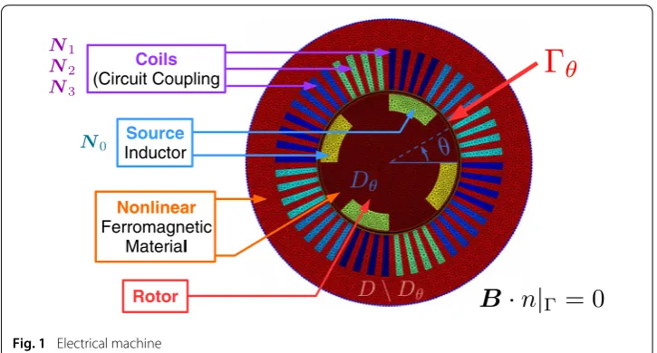
behaviour of the ferromagnetic materials of the rotor and the stator is considered. The domainDNL of boundaryNLsuch thatθ∩NL = ∅gathers all the region with non linear materials. Four stranded inductors are considered. Only one inductor belongs to the subdomainDθ and the others toD\Dθ. We denote byijthe current associated with the coil of thejth phase andi0the current flowing into the inductor of the rotor.
When the rotor is steady, the Maxwell equations describing the magnetostatic field problem reads:
curlH(x)=
3
j=0
ijNj(x) (1)
divB(x)=0 (2)
whereH denotes the magnetic field,Bthe magnetic flux density andNjthe unit current density vector flowing through thejth stranded inductor.
One has to add a constitutive law in order to link theBfield with theHfield:H =νB, withν the magnetic reluctivity. For the isotropic ferromagnetic materials (inDNL), the reluctivity depends on the value of the norm ofB:ν = ν(B). In order to apply a fixed point technique to solve this nonlinear equation, one can introduce a virtual magnetization vectorHfp(B) such that:
H=νfpB+Hfp(B) (3)
Hfp(B)=(ν(B)−νfp)B (4)
To ensure the uniqueness of the solution, boundary conditions have to be added. In this article, we assume that:
B·n=0 on (5)
To solve the previous problem, the vector potential formulation can be used. From (2), the vector potentialAis defined such that:
B(x)=curlA(x) (6)
Then, a strong boundary condition is added:
A×n=0 on (7)
which satisfies (5).
Combining (1), (3), (6) and (7), the vector potential formulation of the nonlinear mag-netostatic problem reads:
curlνfpcurlA(x)=
3
j=0
ijNj(x)−curlHfp(A(x)) (8)
Nonlinear
Ferromagnetic Material Source Inductor Coils (Circuit Coupling
Rotor
Fig. 1 Electrical machine
the vector of sizeNof entries (XA,k)k=1...N. Then, applying the Galerkin method to solve
(8) leads to the following non linear system of equations.
MXA=
3
j=0
Fjij−GNL(XA) (9)
withMthe stiffness matrix of sizeN×Nwhich is symmetric definite, andF andGNL
two vectors of sizeN.
Motion through the overlapping method
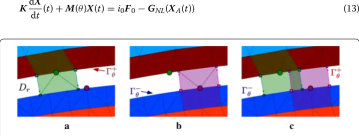
In order to model the rotation of Dθ, the overlapping method is used. This methods allows to take into account the motion of a sub-domain efficiently along a thin non-meshed domain. Therefore, in order to apply this method to our problem, a non-non-meshed domainDris introduced betweenDθandD\Dθof boundariesθ−andθ+respectively, as shown on Fig.2.
Basically, the overlapping method consists in computing interactions betweenDθ and
D\DθinsideDr[24,25]. This can be done by extending the finite element functions of each domain ontoDrby ensuring continuity properties. SinceDris a non-meshed domain, no extra unknowns are added to the problem.
To achieve that, the nodal basis functions of the nodes belonging to θ+ are firstly extended toθ−. For simple boundary surfaces such as circles, this extension is done by
projecting the support of the nodal function along the normal vector of the boundaryθ+, as seen on Fig.3a. Then, Fig.3b shows how the nodal functions of−θ are extended in the same way toθ+. Finally, the support of the nodal functions from+θ intersects with the support of the nodal functions ofθ−, and therefore, an interaction of the two sub-domains can be computed. This interaction area is represented in dashed lines on Fig.3c. More details of this method can be found in [25].
Since the shape functions associated to the nodes alongθ+andθ−now depend on the parameterθ, equation (9) reads:
M(θ)XA=
3
j=0
Fjij−GNL(XA) (10)
under the assumptions thatθ+−∩NL=∅.
Circuit and mechanical coupling
The coupling of the rotating nonlinear magnetostatic problem with circuit and mechanical equations are studied in this section.
Circuit coupling
We suppose that the first inductor is supplied by a direct currenti0and the others are
connected to electric loads composed of resistorsRand inductancesL. In these conditions, the currents{ik , k = 1,. . .,3}are three new unknowns of the problem. Then, circuit equations must be added to the initial problem:
dφk
dt (t)+L dik
dt (t)+Rik(t)=0, ∀k=1,. . .,3 (11) withφkthe linkage magnetic flux associated with thekth inductor. The magnetic fluxes
are express as a function of the vector potential such that:
φk(t)=
DNk(x)·A(x,θ, t)dx=F t
kXA, ∀k=1,. . .,3 (12)
The potentialA is now time-dependent. Therefore, its discrete counterpartXA also depends of the time variablet. Then, by introducingXthe new unknown vector such as X = [XA(t);i1(t);i2(t);i3(t)], the numerical model can be written from (10)–(12) as the
following system of differential algebraic equations:
KdX
dt (t)+M(θ)X(t)=i0F0−GNL(XA(t)) (13)
with K andMsquared matrices of sizeN +3,F andGNL two vectors of sizeN +3.
To solve this system without stability issues, the use of a backward scheme is preferable. Therefore, applying an Euler Backward scheme on (13) with a time-stepτ leads to:
K
τ +M(θ)
Xk = Kτ Xk−1+i
0F0−GNL(XkA) (14)
whereXk=X(t=kτ).
Mechanical coupling
The mechanical coupling links the angular velocity of the rotor= ddθt with the electro-magnetic torqueTEM(A). The mechanical equation reads:
Jd
dt +f=TEM(A)−TMech (15)
with J the inertial momentum of the rotor, f a friction constant andTMech the load. The computation of the electromagnetic torqueTEM(A) derives from the virtual work principle. It can be written as a quadratic function ofA[26]. In a discrete setting, one can write:
TEM(XA)=XtAMTXA (16)
withMT a sparse matrix of sizeN. Applying an explicit Euler scheme on (15) and using (16) leads to the discrete mechanical equation:
k+1=k(1+ fτ
J )+
1
J(XtAMTXA−TMech) (17)
and thenθk+1=θk+τk+1. In the study of electrical machine, the time constantτMech
of the mechanical equation (17) is much larger than the one arising from the circuit couplingτElec. Thus, an explicit time-scheme for (17) is used. Like any explicit method,
the approach is consistent if the time-stepτis chosen sufficiently small in order to capture the dynamics of the system [5,6,27] which is the case in practice since the time-stepτ is chosen according toτElecwhich is much smaller thanτMech.
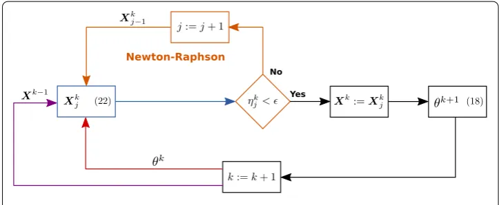
Numerical solution
The nonlinear system of equations (14) can be solved by using a fixed-point approach, or more efficiently, the Newton-Raphson (NR) algorithm. Those methods allow to transform a nonlinear problem into a sequence of linear problems. Therefore, in order to find the nonlinear solutionXk of (14) at the kth step, one has to solve several linear problems of solutionXkj, such that limj→∞Xkj = Xk. When applying the NR algorithm, only few
iterations are required to reach convergence in practice. At thekth time-step, the residual vectorRkof sizeN+3 is defined such that:
Rk(U)= K
τ +M(θk)
U+GNL(U)−K
Moreover, the Jacobian matrix of the problem at thekth time-step is:
Jk(U)= K
τ +M(θk)+JNL(U) (19)
whereJNL(U) denotes the Jacobian operator related to the nonlinear termGNL(.). Then, thejth linear problem from the NR method reads:
Jk(Xkj−1)(Xkj −Xjk−1)= −Rk(Xkj−1) (20)
which allows to computeXkj fromXkj−1. A stop criterion comparingηkj = ||Xkj −Xkj−1|| with a user-defined parameter < 1 is used to determine whether the algorithm has converged or not.
Finally, the different steps describing the numerical scheme of the nonlinear coupled problem are summarized in Fig.4.
Model order reduction methods
The nonlinear coupled problem (14)–(17) has a high computational cost. Indeed, solving the nonlinear equation (14) requires a high number of unknowns and several Newton-Raphson iterations for each time-step. Moreover, adding the mechanical equation (17) to the problem makes the simulation time interval much larger versus the time-stepτ defined from the smallest time constantτElecrelated to the electrical behaviour of the
rotating machine. Moreover, the electromagnetic torqueTEMhas a very high oscillating frequency. Therefore, we propose to apply a MOR approach to the problem (14)–(17) through the proper orthogonal decomposition combined with the (Discrete) empirical interpolation method.
Proper orthogonal decomposition
The POD approach allows to significantly reduce the number of unknowns of the equation system. Indeed, the POD belongs to the projection model order reduction methods which consist in seeking an approximation of the large-scale solutionXr into a small reduced basis.
Projection-based model order reduction
Into the projection-based model order reduction framework, the solutionXkof the non-linear equation (14) is approximated as:
Xk ≈Xk
r (21)
whereXkr denotes the reduced solution and is a “small” vector of sizem, withm<<N. , the reduced basis, is a rectangular matrix inR(N+3)×m.
Injecting (21) into (14) gives the system of equations: K
τ +M(θ)
Xkr = Kτ Xkr−1+i0F0−GNL(Xkr) (22)
However, the latter system is rectangular. Therefore, one can perform a Ritz-Galerkin projection by multiplying (22) witht. Finally, the reduced system of sizemreads:
K r
τ +Mr(θ)
Xkr = KτrXkr−1+i0Fr−GNL,r(Xkr) (23)
with Kr = tK ∈ Rm×m, Mr(θ) = tM(θ) ∈ Rm×m , Fr = tF0 ∈ Rm and
GNL,r(Xkr) = tGNL(Xkr) ∈ Rm. Thus, those equations lead to a reduced Newton-Raphson iteration:
Jk
r(Xkr,j)(Xkr,j+1−Xkr,j)= −Rkr(Xkr,j) (24)
with
Jkr(Xkr,j)= Kτr +Mr(θk)+JNL,r(Xkr,j) Jk
NL,r(Xkr,j)=tJkNL(Xkr,j) Rkr(Xkr,j)=tRk(Xkr,j)
The key of those projection methods is to find a reduced basisfrom which the reduced system (23) provides an approximation of the full system (14) as good as possible.
Determination of the reduced basis through the proper orthogonal decomposition
The proper orthogonal decomposition, introduced in 1967 for fluid mechanic applications [28], is one of the most used model order reduction method [10,11]. This approach requires snapshots, i.e. solutions of the problem for different parameter values, in order to build a reduced basis. Those snapshots can be computed numerically or extracted from experimental data.
Then, given a set oflsnapshotsS= {X1A,X2A,. . .,XlA} ∈RN×l, one has to perform upon it a singular value decomposition (SVD). Letrbe the rank of the matrixSwithr<land
r<N, then the SVD of the snapshot matrix is written:
S=U1U2
0
0 0
Vt
1
Vt
2
whereU1andV1are matrices inRN×randRl×rrespectively, whose columns are
ortho-normal (Ut1U1=Vt1V1=Ir).is a diagonal matrix of sizerwhich contains the so-called singular values{σi, i=1. . .r}such thatσ1> σ2>· · ·> σr>0. Thus, the reduced basis which allows to approximateXAisA=U1.
Truncation of the reduced basis
Truncation plays an essential part on methods like the POD which are based on the SVD. Indeed, we have seen that the SVD allows to find the rankrof the snapshot matrixSin (25). However for numerical problems, the snapshot matrixSis likely to be full rank since its singular values are never equal to the spurious zero because of the numerical noise.
Therefore, it is often advised to truncate the basis, i.e. to reduce the size of the reduced basis, according to a truncation criterion. In the literature, several methods have been proposed.
A very popular approach consists in keeping thepfirst modes amongstlwhich corre-spond to singular values larger than a user-defined small constant :
A=U1(:,1. . .p)/σi> , i=1. . .p
An other truncation method proceeds by considering the cumulative sum so that it verifies for a fixed :
A=U1(:,1. . .p)/
1−
p i=1σi
l i=1σi
<
In this paper, a truncation based on the orthogonality condition is used. Indeed, the matrixM⊥=Ut1U1withU1given by (25) should be equal to the identity matrix of sizer.
However, due to numerical computations and noise, this equality does not hold andM⊥ is not diagonal:
M⊥=M ⇒M⊥=Ir
However, the matrixM⊥is almost diagonal with magnitude 1 for the firstpmodes but produce extra-diagonal terms for the last modes:
M ≈
Ip 1
t
1 2
with
1=0
2=Ir−p
This means that the smaller the singular value is, theless orthogonalits corresponding mode is, which implies that the less relevant the mode is. Therefore, we propose to use the following truncation approach, based on the value of:
Structure preserving approach
SinceXis made from two different sets of unknowns,XAand the currents [i1(t), i2(t), i3(t)],
a structure-preserving approach is used. Basically, it consists in constructing reduced basis for each kind of unknowns. However, since the number of circuit coupling equations remains small versus the number of nodesN, only the unknownsXAare approximated in a reduced basis. Therefore, the full reduced basisfrom (21) is written:
=
A 0 0 Ini
(26)
withInidefining the identity matrix of sizeni.
(Discrete) Empirical interpolation method
Although the number of unknowns has been dramatically reduced though the POD approach, the computational cost of the nonlinear termGNL,r(Xkr) remains prohibitive.
Indeed, one has to express first this quantity in the full basis, and secondly, project it onto the reduced basis. Therefore, we propose to apply the (Discrete) empirical interpolation method which allows to compute some nonlinear terms only on DEIM-chosen points, and then to interpolate the remaining entries ofGNL.
Given a snapshot collectionSNLof the nonlinear termGNL, a POD basisNL ∈RN×s
is calculated using the same approach as the one presented in the previous section. Then, the (D)EIM algorithm [18] allows to generate a selection matrixP=[ec1,. . .,ecr]∈RN×s where{ecj, j=1. . .r}denotes the unit vector associated to thecjthcomponent. Then, the nonlinear term is approximated as:
GNL(U)=NLPtNL−1PtGNL(U) (27)
while the algorithm ensures that PtNL is invertible. Thus, only PtGNL(U) has to be computed. For finite element problems, the value of any vector at a certain point only depend on itself and its neighbours. Then, the computational cost ofPtGNL(U) is highly
reduced compared with the one ofGNL(U).
Furthermore, one may apply the POD projection onto the (D)EIM approximation. Therefore, the POD-(D)EIM approximation of the nonlinear terms reads:
GNL,r(U)=tNL PtNL−1PtGNL(U) (28)
and the nonlinear Jacobian associated to the (D)EIM approximation is:
JNL,r(U)=tNL PtNL−1PtJNL(U) (29)
Note that the matrixtNLin (28–29) is of sizer×swithr<<Nands<<N.
Applications
A 2D model of a nonlinear synchronous generator is studied. The geometry and the mesh of the domain are presented in the Fig.1. The rotor is driven by a constant torqueTMech
and is supplied with a direct currenti0. Moreover, the motion of the rotor is taken into
Since the time constant of the mechanical equation (17) is much larger than the one arising from the circuit equation (11), a high number of time-steps is required to reach the steady state. In our example, we havent =104time-steps. The 2D mesh of this machine is made of 23,492 triangles and 12,097 nodes.
Model order reduction strategy
In order to build an accurate reduced system, a collection of snapshots has to be chosen in such a way that they contain most of the different behaviours of the system. For our problem, we impose that at least, the snapshots collect a full mechanical period so that the reduced basis contains an entire rotation. Thus, applying a “direct” reduction approach where one collects the snapshots during the firstmtime-steps and then begin the reduced scheme at the (m+1)th time-step may lead to a high computational cost. Indeed, in our settings, a full mechanical period requires approximately 2000 time-steps.
Moreover, applying a greedy procedure to constructmbasis vectors over the full time interval would require solvingmtimes the reduced system on every time-step, which is also very resource-demanding.
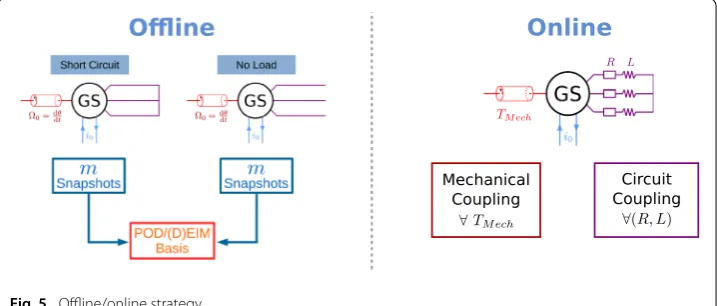
However, in the field of electrical engineering, a synchronous machine is easily char-acterized through two simple tests procedures: a no-load and a short-circuit test. During those tests, there are no more mechanical coupling: the rotation speed is set to a constant value0. Thus, the electromagnetic torqueTEMof high oscillating frequency is no more
related to the problem, and allows to take a quite important time-step in order to compute a full mechanical rotation with a reduced number of snapshots (in our case 122). Further-more, the short-circuit test considers the case where both the value ofRandLis zero in the circuit equation (11) whereas the no-load case consists in not taking into account the circuit coupling. Therefore, the only parameter left in those two test cases is the rotation angleθ.
Finally, those two sets of snapshots are used to construct a dynamic reduced system which accurately approximate the electrical machine, for any value ofR,LandTMechin (11) and (17). The MOR strategy is summarized on Fig.5.
Offline procedure
Each of the two tests procedures has been computed withm=122 snapshots uniformly distributed in [0,2π] with respect to the rotation angle:θk = 2121kπ, k=0. . .121. One has
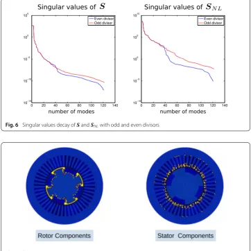
to note that the half of the electrical machine presents symmetry conditions. Therefore, in order to maximize the information collected in the snapshots, one has to make sure that the divisor inθk(i.e. 121 in our case) is odd. Indeed, taking even divisor implies gath-ering snapshots which have symmetry conditions and therefore redundant information. In practice, this redundancy is highlighted by observing the slope of the singular values obtained from the snapshotsSandSNL, according to (25): the steepest it is, the less rele-vant the snapshots are. This is shown on Fig.6where the singular values are plotted for snapshots computed with odd divisor (θk = 121) and even divisor (θk = 120). Indeed, above 40 modes approximately, the singular values of the even divisor case are at least one order of magnitude smaller than the odd divisor case.
The 2×122=244 snapshots obtained from the two tests procedures are concatenated in order to build the two reduced basis andNL. The truncation has been applied according to the orthogonality criterion (“Truncation of the reduced basis” section) with =10−7. Finally, the two reduced basisandNLare respectively of size 71 and 160. Figure7shows the interpolation points selected by the (D)EIM algorithm. One can see that the (D)EIM points are located around the air gap for the stator and the rotor. This is relevant since the magnetic field magnitude varies much more on the surface of the rotor and also on the stator tooth tips than inside the rotor and in the stator yoke and teeth.
Fig. 6 Singular values decay ofSandSNLwith odd and even divisors
Online procedure
Once the reduced system has been built, the online computation involving the mechanical and the circuit coupling is performed by applying a constant torqueTMech= 47N.min
(15) on 104time-steps.
Verification
The reduced system is tested on a short-circuit case and a no-load case, but with a mechan-ical coupling. The results are compared with a full FEM model. Figure8shows the evolu-tions of the electromotive force (EMF) at the terminals of each inductors of the stator. The EMF are computed by the derivative of the magnetic linkage fluxes. For both tests, the EMF evolutions obtained from the reduced model are close to those from the full model.
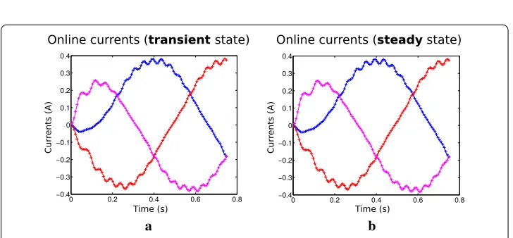
Adaptivity of the reduced basis
The reduced model is tested with different values of Rand L in the circuit equation (11). The evolutions of the currents obtained from the reduced model and the full model associated with the stranded inductors of the stator are presented on Figs.9,10,11,12 and13. We can see that the currents from the reduced model are close to the references. This implies that the reduced system is dynamic in the sense that it adapts to values of
RandLfor which no snapshots were computed. By taking into account the snapshots computation, the speedup obtained with model order reduction is approximately 35.
a b
c d
a b
Fig. 9 Currents computed with the FEM and the MOR approaches for an online computation withR=5k andL=2Hduring the transient state (a) and the steady state (b)
a b
Fig. 10 Currents computed with the FEM and the MOR approaches for an online computation with
R=600andL=0Hduring the transient state (a) and the steady state (b)
a b
Fig. 11 Currents computed with the FEM and the MOR approaches for an online computation with
R=10kandL=0Hduring the transient state (a) and the steady state (b)
Conclusions
a b
Fig. 12 Currents computed with the FEM and the MOR approaches for an online computation withR=0 andL=0.5Hduring the transient state (a) and the steady state (b)
a b
Fig. 13 Currents computed with the FEM and the MOR approaches for an online computation withR=0 andL=5Hduring the transient state (a) and the steady state (b)
nonlinear problem has been solved by using the Newton-Raphson approach and the motion of the rotor with the overlapping finite element method. In order to obtain an efficient reduced model on the whole operating range of electrical machines, an empirical “Offline/Online” approach has been developed. With the proposed approach, the start-up of a synchronous machine until it reaches the steady state has been studied. On this example, the reduced model appears to be more efficient with respect to the computation cost than the reference model especially when the time-step is very small. In terms of accuracy, the global quantities can be approximated with a low number of unknowns and thus, the computation time is significantly reduced. Our future works will focus on POD-(D)EIM error estimators in order to build robust and adaptive reduced systems of electrical machines.
Authors’ contributions
The four authors have developed the theory part. LM has carried out the numerical implementation and has drafted the manuscript. TH, SC and BG have supervised the different studies and the corrections of the draft. All authors read and approved the final manuscript.
Author details
d’Electrotechnique et d’Electronique de Puissance, Univ. Lille, Laboratoire L2EP, Cité Scientifique, Bâtiment P2, 59655 Villeneuve d’Ascq, France.
Acknowledgements None.
Competing interests
The authors declare that they have no competing interests.
Received: 7 December 2015 Accepted: 24 February 2016
References
1. Ho SL, Fu WN. A comprehensive approach to the solution of direct-coupled multislice model of skewed rotor induction motors using time-stepping eddy-current finite element method. IEEE Transact Magn. 1997;33(3):2265–73. 2. Demenko A, Dolinar D, Hameyer K, Nowak L, Zawirski K, Krebs G, Tounzi A, Piriou F, Pauwels B, Willemot D. Design and study of a linear actuator using an analytical approach and the 3D FEM. Int J Comput Math Electr Electr Eng. 2007;26(4):1005–16.
3. Demenko Andrzej, Hameyer Kay, Nowak Lech, Zawirski Krzysztof, Shi Xiaodong, Le Menach Yvonnick, Ducreux Jean-Pierre, Piriou Francis. Comparison of slip surface and moving band techniques for modelling movement in 3D with FEM. Int J Comput Math Electr Electr Eng. 2006;25(1):17–30.
4. Taibi Saoudi, Tounzi Abdelmounaïm, Piriou Francis. Study of a stator current excited vernier reluctance machine. Energy Convers IEEE Transact. 2006;21(4):823–31.
5. Henrotte F, Nicolet A, Hedia H, Genon A, Legros W. Modelling of electromechanical relays taking into account movement and electric circuits. IEEE Transact Magn. 1994;30(5):3236–9.
6. Albunni MN, Rischmuller V, Fritzsche T, Lohmann B. Model-order reduction of moving nonlinear electromagnetic devices. IEEE Transact Magn. 2008;44(7):1822–9.
7. Henneron Thomas, Clénet Stéphane. Model order reduction of quasi-static problems based on POD and PGD approaches. Eur Phys J Appl Phys. 2013;64(02):24514.
8. Nouy Anthony. A priori model reduction through proper generalized decomposition for solving time-dependent partial differential equations. Comput Methods Appl Mech Eng. 2010;199(23):1603–26.
9. Chinesta F, Leygue A, Bordeu F, Aguado JV, Cueto E, Gonzalez D, Alfaro I, Ammar A. PGD-based computational vademecum for efficient design, optimization and control. Arch Comput Methods Eng. 2013;20(1):31–59. 10. Anthanasios AC, Sorensen DC, Gugercin S. A survey of model reduction methods for large-scale systems. Contemp
Math. 2001;280:193–220.
11. Jolliffe I. Principal component analysis. Wiley; 2002.
12. Odabasioglu A, Celik M, Pileggi LT. PRIMA: passive reduced-order interconnect macromodeling algorithm. In Proceed-ings of the 1997 IEEE/ACM international conference on Computer-aided design. IEEE Computer Society. 1997;58–65. 13. Bui-Thanh T, Damodaran M, Willcox K. Proper orthogonal decomposition extensions for parametric applications in
compressible aerodynamics. AIAA paper. 2013; 4213.
14. Ladeveze P, Passieux JC, Neron D. The latin multiscale computational method and the proper generalized decompo-sition. Comput Methods Appl Mech Eng. 2010;199(21):1287–96.
15. Henneron T, Clenet S. Application of the PGD and DEIM to solve a 3D non-linear magnetostatic problem coupled with the circuit equations. Magn IEEE Transact. 2015; 99.
16. Galbally D, Fidkowski K, Willcox K, Ghattas O. Non-linear model reduction for uncertainty quantification in large-scale inverse problems. Int J Numer Methods Eng. 2010;81(12):1581–608.
17. Barrault M, Maday Y, Nguyen NC, Patera AT. An ‘empirical interpolation’ method: application to efficient reduced-basis discretization of partial differential equations. Comptes Rendus Mathematique. 2004;339(9):667–72.
18. Chaturantabut S, Sorensen DC. Nonlinear model reduction via discrete empirical interpolation. SIAM J Sci Comput. 2010;32(5):2737–64.
19. Hinze M, Kunkel M. Discrete empirical interpolation in POD model order reduction of drift-diffusion equations in electrical networks. In scientific computing in electrical engineering SCEE 2010. Springer; 2012. p. 423–31. 20. ¸Stef˘anescu R, Navon Ionel Michael. POD/DEIM nonlinear model order reduction of an ADI implicit shallow water
equations model. J Comput Phys. 2013;237:95–114.
21. Ghasemi M, Yang Y, Gildin E, Efendiev Y, Calo VM. Fast multiscale reservoir simulations using pod-deim model reduction. In SPE reservoir simulation symposium, 2015.
22. Pierquin A, Henneron T, Clénet S, Brisset S. Model-order reduction of magnetoquasi-static problems based on POD and Arnoldi-based Krylov methods. IEEE Transact Magn. 2015;51(3):1–4.
23. Henneron Thomas, Clenet Stephane. Model order reduction of non-linear magnetostatic problems based on POD and DEI methods. IEEE Transact Magn. 2014;50(2):33–6.
24. Tsukerman IA. Overlapping finite elements for problems with movement. IEEE Transact Magn. 1992;28(5):2247–9. 25. Krebs G, Henneron T, Clenet S, Le Bihan Y. Overlapping finite elements used to connect non-conforming meshes in
3-D with a vector potential formulation. IEEE Transact Magn. 2011;47(5):1218–21.
26. Ren Z, Razek A. Local force computation in deformable bodies using edge elements. IEEE Transact Magn. 1992;28(2):1212–5.