Adv. Radio Sci., 9, 145–152, 2011 www.adv-radio-sci.net/9/145/2011/ doi:10.5194/ars-9-145-2011
© Author(s) 2011. CC Attribution 3.0 License.
Advances in
Radio Science
Fast beampattern evaluation by polynomial rooting
P. H¨acker, S. Uhlich, and B. Yang
Chair of System Theory and Signal Processing, Universit¨at Stuttgart, Pfaffenwaldring 47, 70550 Stuttgart, Germany
Abstract. Current automotive radar systems measure the distance, the relative velocity and the direction of objects in their environment. This information enables the car to sup-port the driver.
The direction estimation capabilities of a sensor array de-pend on its beampattern. To find the array configuration lead-ing to the best angle estimation by a global optimization algo-rithm, a huge amount of beampatterns have to be calculated to detect their maxima. In this paper, a novel algorithm is proposed to find all maxima of an array’s beampattern fast and reliably, leading to accelerated array optimizations. The algorithm works for arrays having the sensors on a uniformly spaced grid. We use a general version of the gcd (greatest common divisor) function in order to write the problem as a polynomial. We differentiate and root the polynomial to get the extrema of the beampattern. In addition, we show a method to reduce the computational burden even more by decreasing the order of the polynomial.
1 Introduction
A common problem in signal estimation theory is the esti-mation of objects’ direction (DOA, direction of arrival) using an array of sensors. In far range automotive radar systems, we are facing narrow-band and far field conditions. In ad-dition, a Pulse-Doppler or frequency modulated continuous wave radar deals most of the time with the single object case, because all objects are first separated in range and velocity. Only objects with the same range and velocity have to be sep-arated in DOA. We consider the case of azimuth estimation only since it is much more important than elevation in au-tomotive applications. Together with the distance estimates, the azimuth angle determines the position of the relevant
ob-Correspondence to: P. H¨acker
ject uniquely relative to the vehicle. Using this information, the car can act in an intelligent way. Two examples of this behavior are ACC (Jurgen, 2006) (Adaptive Cruise Control) and LCA (Ruder et al., 2002) (Lane Change Assistant).
For mass production, a sensor array has to be cheap. Hence the number of sensor elements is limited. Neverthe-less, the DOA estimates have to be as accurate as possible. For a fixed DOA estimation algorithm, the positions of the sensors have to be optimized, to get the best DOA estimates according to a suitable criterion.
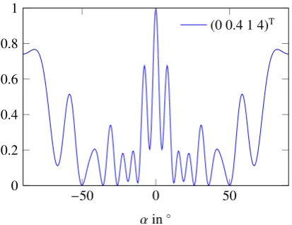
A frequently used optimization criterion is the Cramr-Rao bound (Athley et al., 2004), which is a lower bound on the variance of any unbiased estimator. The Cramr-Rao bound only takes local DOA errors into account (Athley, 2005). Local errors are errors smaller than half the size of the ar-ray’s main lobe. Unfortunately, with a cheap sensor and thus few snapshots and low SNR, global errors are not negligi-ble. Athley (2005) approximated the global errors analyti-cally and calculated an error probability per side lobe of the so called beampattern. This allows the analytical calculation of the variance of DOA estimates, which can be used as a cost function for array optimization. A typical beampattern is shown in Fig. 1.
This approach has two shortcomings: First, the maximum of each side lobe has to be computed numerically. So one needs a fast and reliable algorithm to find all local maxima of the beampattern. Second, the variance function does a weighting preferring smaller errors. Having small local er-rors is obviously useful, but at least in automotive applica-tions, having a DOA error of 10◦is not better than having an error of 20◦. Larger errors can even be advantageous, as they are easier to classify as outliers and to reject over time by using tracking.
These considerations lead to a minimization of global er-rors, where only the height of the side lobes is important and not their position. Because of the huge gradient in Athley’s error probability (Fig. 2) it is reasonable to assume, that min-imizing the maxima of the side lobes will lead close to the
146 P. H¨acker et al.: Fast beampattern evaluation by polynomial rooting
Manuscript prepared for Adv. Radio Sci.
with version 3.2 of the L
ATEX class copernicus.cls.
Date: 30 May 2011
Fast Beampattern Evaluation by Polynomial Rooting
Patrick H¨acker, Stefan Uhlich, and Bin Yang
Chair of System Theory and Signal Processing, Universit¨at Stuttgart, Pfa
ff
enwaldring 47, 70550 Stuttgart, Germany
Abstract.
Current automotive radar systems measure the
distance, the relative velocity and the direction of objects
in their environment. This information enables the car to
support the driver. The direction estimation capabilities of
a sensor array depend on its beampattern. To find the
ar-ray configuration leading to the best angle estimation by a
global optimization algorithm, a huge amount of
beampat-terns have to be calculated to detect their maxima. In this
paper, a novel algorithm is proposed to find all maxima of an
array’s beampattern fast and reliably, leading to accelerated
array optimizations. The algorithm works for arrays having
the sensors on a uniformly spaced grid. We use a general
ver-sion of the gcd (greatest common divisor) function in order
to write the problem as a polynomial. We di
ff
erentiate and
root the polynomial to get the extrema of the beampattern.
In addition, we show a method to reduce the computational
burden even more by decreasing the order of the polynomial.
1
Introduction
A common problem in signal estimation theory is the
esti-mation of objects’ direction (DOA, direction of arrival) using
an array of sensors. In far range automotive radar systems,
we are facing narrow-band and far field conditions. In
ad-dition, a Pulse-Doppler or frequency modulated continuous
wave radar deals most of the time with the single object case,
because all objects are first separated in range and velocity.
Only objects with the same range and velocity have to be
sep-arated in DOA. We consider the case of azimuth estimation
only since it is much more important than elevation in
au-tomotive applications. Together with the distance estimates,
the azimuth angle determines the position of the relevant
ob-ject uniquely relative to the vehicle. Using this information,
Correspondence to:
Patrick H¨acker
([email protected])
−50 0 50
0 0.2 0.4 0.6 0.8 1
αin◦
(0 0.4 1 4)T
Fig. 1.Beampattern with main lobe atα=0 and several side lobes
the car can act in an intelligent way. Two examples of this
behavior are ACC [Jurgen (2006)] (Adaptive Cruise Control)
and LCA [Ruder et al. (2002)] (Lane Change Assistant).
For mass production, a sensor array has to be cheap.
Hence the number of sensor elements is limited.
Neverthe-less, the DOA estimates have to be as accurate as possible.
For a fixed DOA estimation algorithm, the positions of the
sensors have to be optimized, to get the best DOA estimates
according to a suitable criterion.
A frequently used optimization criterion is the
Cram´er-Rao bound [Athley et al. (2004)], which is a lower bound
on the variance of any unbiased estimator. The
Cram´er-Rao bound only takes local DOA errors into account [Athley
(2005)]. Local errors are errors smaller than half the size of
the array’s main lobe. Unfortunately, with a cheap sensor and
thus few snapshots and low SNR, global errors are not
negli-gible. Athley [Athley (2005)] approximated the global errors
analytically and calculated an error probability per side lobe
of the so called beampattern. This allows the analytical
cal-culation of the variance of DOA estimates, which can be used
as a cost function for array optimization. A typical
beampat-Fig. 1. Beampattern with main lobe atα=0 and several side lobes.
optimum, as only the highest side lobe has a significant er-ror probability. The erer-ror probability in Fig. 2 is derived for white noise. If this condition is violated by clutter or another object, the error probability is much higher.
The criterion has to be calculated for a huge number of arrays during the array optimization. In this paper, we will not investigate which global optimization algorithm to use. Instead we focus on the fast calculation of beampatterns. We introduce the beampatterns in Fig. 2 and derive needed math-ematics in Sect. 3. The fast evaluation of the cost functions are shown in Sect. 4, having Eq. (5) as the most important equation. We present improvements of this basic algorithm for our specific problem in Sect. 5. We show some results in Sect. 6 and conclude our work in Sect. 7.
2 Beampatterns
We assume that all N sensors differ only in their posi-tions having identical (e.g. omnidirectional) characteristics. If their characteristics differ only slightly, the following re-sults will be approximately be true and are still of value. If the characteristics are completely different, the proposed al-gorithm cannot be used.
As we want to estimate only the azimuth angle, the sen-sors can all be placed along a horizontal line orthogonal to the driving direction. Without loss of generality, we choose the first sensor of the array as the reference element at po-sition 0. Letp=(p1 ... pN)T be a vector containing the
positions of the sensors normalized by the wavelength. For the following algorithm,pmay only contain rationals, pos-sibly after factorization of a common irrational factor. The steering vectora(u)of lengthN can then be written as
a(u)=√1 N
1 ej2πp1u ··· ej2πpNuT, (1)
withu=sin(α), whereαis the broadside azimuth angle.
2
:
0.6 0.7 0.8 0.9 1 10−13
10−9 10−5 10−1
height of side lobe relative to main lobe
error
probability 12 dB SNR 13 dB SNR 14 dB SNR 15 dB SNR
Fig. 2.Error probability for single side lobe
tern is shown in Fig. 1.
This approach has two shortcomings: First, the maximum
of each side lobe has to be computed numerically. So one
needs a fast and reliable algorithm to find all local maxima
of the beampattern. Second, the variance function does a
weighting preferring smaller errors. Having small local
er-rors is obviously useful, but at least in automotive
applica-tions, having a DOA error of 10
◦is not better than having
an error of 20
◦. Larger errors can even be advantageous, as
they are easier to classify as outliers and to reject over time
by using tracking.
These considerations lead to a minimization of global
er-rors, where only the height of the side lobes is important and
not their position. Because of the huge gradient in Athley’s
error probability (Fig. 2) it is reasonable to assume, that
min-imizing the maxima of the side lobes will lead close to the
optimum, as only the highest side lobe has a significant
er-ror probability. The erer-ror probability in Fig. 2 is derived for
white noise. If this condition is violated by clutter or another
object, the error probability is much higher.
The criterion has to be calculated for a huge number of
arrays during the array optimization. In this paper, we will
not investigate which global optimization algorithm to use.
Instead we focus on the fast calculation of beampatterns.
We introduce the beampatterns in Sect. 2 and derive needed
mathematics in Sect. 3. The fast evaluation of the cost
func-tions are shown in Sect. 4, having Eq. (5) as the most
im-portant equation. We present improvements of this basic
al-gorithm for our specific problem in Sect. 5. We show some
results in Sect. 6 and conclude our work in Sect. 7.
2
Beampatterns
We assume that all
N
sensors di
ff
er only in their
posi-tions having identical (e.g. omnidirectional) characteristics.
If their characteristics di
ff
er only slightly, the following
re-sults will be approximately be true and are still of value. If
the characteristics are completely di
ff
erent, the proposed
al-gorithm cannot be used.
As we want to estimate only the azimuth angle, the sensors
can all be placed along a horizontal line orthogonal to the
driving direction. Without loss of generality, we choose the
first sensor of the array as the reference element at position
0. Let
p
=
(
p
1...
p
N)
Tbe a vector containing the positions of
the sensors normalized by the wavelength. For the following
algorithm,
p
may only contain rationals, possibly after
fac-torization of a common irrational factor. The steering vector
a
(
u
) of length
N
can then be written as
a
(
u
)
=
√
1
N
1 e
j2πp1u···
e
j2πpNuT,
(1)
with
u
=
sin(
α
), where
α
is the broadside azimuth angle.
Based on those assumptions, we can derive a general
beampattern
b
(
u
;
u
0,
y
) by correlating the steering vector
a
(
u
)
with that for a DOA value
u
0:b
(
u
;
u
0,
y
)
=
a
H(
u
0)a
(
u
)
2=
1
+
P
Nk=1
e
j2πpk(u−u0)
+
e
−j2πpk(u−u0)+
P
Nm=1
e
j2π(pk−pm)(u−u0)
!
N
2(2)
u
can be seen as the direction of the object and
u
0as the test
direction. Using Eq. (2), the beampatterns needed for
[Ath-ley (2005)] as mentioned in the introduction can be
calcu-lated.
The correlation of the steering vectors corresponds to the
similarity of the array responses from the appropriate
direc-tions. The Similarity of steering vectors can lead to
ambigui-ties in the angle estimation. Note, that Eq. (2) can be written
as a one-dimensional function, as all values only depend on
the di
ff
erence of
u
and
u
0. Two special cases areexception-ally important.
In automotive and most other applications, the array
should often uniquely di
ff
er an object in front (
u
0=
0) from
every other angle. This is useful for applications like ACC.
The beampattern becomes then
b
(
u
;0
,
y
)
=
1
+
P
Nk=1
e
j2πpku
+
e
−j2πpku+
P
Nm=1
e
j2π(pk−pm)u
!
N
2(3)
Sometimes every array response from one angle should
di
ff
er from the response from all other angles. This is
espe-cially important in applications like LCA. This condition can
be formulated as
b
(
u
;
−
u
,
y
)
=
1
+
P
Nk=1
e
j4πpku
+
e
−j4πpku+
P
Nm=1
e
j4π(pk−pm)u
!
N
2.
(4)
The result of Eq. (4) can also be achieved by letting
u
→
2
u
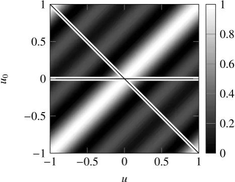
in Eq. (3). In Fig. 3 all possible beampatterns according to
Eq. (2) are shown. The horizontal line denotes the
beampat-tern resulting from Eq. (3). All maxima are included in the
diagonal line following Eq. (4).
Fig. 2. Error probability for single side lobe.
Based on those assumptions, we can derive a general beampattern b(u;u0,y) by correlating the steering vector
a(u)with that for a DOA valueu0:
b(u;u0,y)=
a
H(u 0)a(u)
2 = 1+ N P
k=1
ej2πpk(u−u0)+e−j2πpk(u−u0)+
N
P
m=1
ej2π(pk−pm)(u−u0)
N2
(2) ucan be seen as the direction of the object andu0as the test
direction. Using Eq. (2), the beampatterns needed for Athley (2005) as mentioned in the introduction can be calculated.
The correlation of the steering vectors corresponds to the similarity of the array responses from the appropriate direc-tions. The Similarity of steering vectors can lead to ambigui-ties in the angle estimation. Note, that Eq. (2) can be written as a one-dimensional function, as all values only depend on the difference ofuandu0. Two special cases are
exception-ally important.
In automotive and most other applications, the array should often uniquely differ an object in front (u0=0) from
every other angle. This is useful for applications like ACC. The beampattern becomes then
b(u;0,y)= 1+
N
P
k=1
ej2πpku+e−j2πpku+
N
P
m=1
ej2π(pk−pm)u
N2
(3) Sometimes every array response from one angle should differ from the response from all other angles. This is espe-cially important in applications like LCA. This condition can be formulated as
b(u;−u,y)= 1+
N
P
k=1
ej4πpku+e−j4πpku+
N
P
m=1
ej4π(pk−pm)u
N2 .(4)
P. H¨acker et al.: Fast beampattern evaluation by polynomial rooting 147
:
3
−
1
−
0
.
5
0
0
.
5
1
−
1
−
0
.
5
0
0
.
5
1
u
u
00
0
.
2
0
.
4
0
.
6
0
.
8
1
Fig. 3.
Possible beampatterns and used ones
−
1
−
0
.
5
0
0
.
5
1
0
0
.
2
0
.
4
0
.
6
0
.
8
1
u
b
u
;(0
0
.
4
1
.
7
4
.
3)
TFig. 4.
Beampattern having closely spaced extrema
We want to have the extrema of a continuous signal,
i.e. their positions, their types and their values in a specific
interval. A simple method would be sampling the
continu-ous signal by calculating values in uniform distance
u
∆,
de-termining coarse extrema by comparison of neighbor
sam-ples and performing a local optimization on each coarse
ex-tremum. The problem with this approach is that two extrema
can be very tight. This happens when two extrema converge
to a saddle point by changing the sensors’ positions. In Fig. 4
an example of extrema (magenta, dashed) being closer than
the sampling distance (green, dotted) is shown. That’s why
the sampling frequency must be much higher than
1/
u∆to
make only few errors. Alternatively, we could do a local
optimization starting from every sample, even though this is
definitely slow. Although most maxima are found with that
approach, there are some exceptions. This can be rapidly
ver-ified with Eq. (4) and
p
=
(0 0
.
5 11)
Taround
u
=
0
.
5. Thus
a sampling algorithm cannot be fast and free of errors at the
same time.
3
Generalized gcd
Before having a closer look into the algorithm we need to
generalize the gcd and therefore the lcm. The classical gcd
is the greatest common divisible
integer
of
two integers
,
whereas the classical lcm is the least common multiple
in-teger
of
two integers
. The lcm can be computed e
ffi
ciently
with Euclid’s or Stein’s algorithm [Cormen et al. (2001)].
The gcd can be calculated using the lcm [Rosen and Michaels
(2000)]. We now want to generalize the emphasized terms.
3.1
gcd
/
lcm of multiple integers
Let us generalize the gcd of multiple integers
i
1,
i
2,
i
3,
i
4(lcm
analog):
gcd(
i
1,
i
2,
i
3,
i
4)
=
gcd(gcd(
i
1,
i
2)
,
gcd(
i
3,
i
4))
This e
ff
ectively transforms the problem of multiple integers
into the recursive gcd calculation of two integers. The gcd of
a vector
p
is gcd(
p
)
=
gcd(
p
1,...,
p
N−1)
3.2
gcd of two rationals
We want to use gcd with rationals
r
1,
r
2. Note, that all fixed
and floating point numbers in a computer are rationals, so this
is a very general case from a practical point of view. We will
define the generalized gcd by giving an algorithm to compute
it. The algorithm consists of three steps:
1. Convert the floating-
/
fixed-point numbers into fractions
e.g. by regular continued fraction expansion or
gener-alized continued fraction expansion [Rockett and Sz¨usz
(1992)]:
r
1=
n
d
1 1,
r
2=
n
2d
22. Expand the fractions from step 1 so they have a common
denominator, by using the classical lcm (preferably with
intermediate results from continued fractions):
r
1=
(lcm(d1,d2)n1)
/
d1lcm(
d
1,
d
2)
,
r
2=
(lcm(d1,d2)n2)
/
d2lcm(
d
1,
d
2)
3. Calculate the classical gcd of the numerators and divide
by the common denominator from step 2:
gcd(
r
1,
r
2)
=
gcd(
(lcm(d1,d2)n1)
/
d1,
(lcm(d1,d2)n2)/
d2)
lcm(
d
1,
d
2)
As an example, it is
gcd(0
.
1
,
0
.
25)
=
gcd
1
10
,
1
4
!
=
gcd
2
20
,
5
20
!
=
gcd(2
,
5)
20
=
1
20
=
0
.
05
.
During the paper, the generalized gcd function is used with
an arbitrary number of rationals.
Fig. 3. Possible beampatterns and used ones.
The result of Eq. (4) can also be achieved by lettingu→ 2uin Eq. (3). In Fig. 3 all possible beampatterns according to Eq. (2) are shown. The horizontal line denotes the beam-pattern resulting from Eq. (3). All maxima are included in the diagonal line following Eq. (4).
We want to have the extrema of a continuous signal, i.e. their positions, their types and their values in a specific interval. A simple method would be sampling the continu-ous signal by calculating values in uniform distanceu1,
de-termining coarse extrema by comparison of neighbor sam-ples and performing a local optimization on each coarse ex-tremum. The problem with this approach is that two extrema can be very tight. This happens when two extrema converge to a saddle point by changing the sensors’ positions. In Fig. 4 an example of extrema (magenta, dashed) being closer than the sampling distance (green, dotted) is shown. That’s why the sampling frequency must be much higher than1/u1 to
make only few errors. Alternatively, we could do a local op-timization starting from every sample, even though this is definitely slow. Although most maxima are found with that approach, there are some exceptions. This can be rapidly ver-ified with Eq. (4) andp=(0 0.5 11)Taroundu=0.5. Thus a sampling algorithm cannot be fast and free of errors at the same time.
3 Generalized gcd
Before having a closer look into the algorithm we need to generalize the gcd and therefore the lcm. The classical gcd is the greatest common divisible integer of two integers, whereas the classical lcm is the least common multiple
in-teger of two inin-tegers. The lcm can be computed efficiently
with Euclid’s or Stein’s algorithm (Cormen et al., 2001). The gcd can be calculated using the l cm (Rosen and Michaels, 2000). We now want to generalize the emphasized terms.
:
3
−1 −0.5 0 0.5 1
−1
−0.5 0 0.5 1
u u0
0 0.2 0.4 0.6 0.8 1
Fig. 3.Possible beampatterns and used ones
−1 −0.5 0 0.5 1
0 0.2 0.4 0.6 0.8 1 u b u;(0 0 . 4 1 . 7 4 . 3) T
Fig. 4.Beampattern having closely spaced extrema
We want to have the extrema of a continuous signal,
i.e. their positions, their types and their values in a specific
interval. A simple method would be sampling the
continu-ous signal by calculating values in uniform distance
u∆
,
de-termining coarse extrema by comparison of neighbor
sam-ples and performing a local optimization on each coarse
ex-tremum. The problem with this approach is that two extrema
can be very tight. This happens when two extrema converge
to a saddle point by changing the sensors’ positions. In Fig. 4
an example of extrema (magenta, dashed) being closer than
the sampling distance (green, dotted) is shown. That’s why
the sampling frequency must be much higher than
1/
u∆to
make only few errors. Alternatively, we could do a local
optimization starting from every sample, even though this is
definitely slow. Although most maxima are found with that
approach, there are some exceptions. This can be rapidly
ver-ified with Eq. (4) and
p
=
(0 0
.
5 11)
Taround
u
=
0
.
5. Thus
a sampling algorithm cannot be fast and free of errors at the
same time.
3
Generalized gcd
Before having a closer look into the algorithm we need to
generalize the gcd and therefore the lcm. The classical gcd
is the greatest common divisible
integer
of
two integers
,
whereas the classical lcm is the least common multiple
in-teger
of
two integers
. The lcm can be computed e
ffi
ciently
with Euclid’s or Stein’s algorithm [Cormen et al. (2001)].
The gcd can be calculated using the lcm [Rosen and Michaels
(2000)]. We now want to generalize the emphasized terms.
3.1
gcd
/
lcm of multiple integers
Let us generalize the gcd of multiple integers
i
1,
i
2,
i
3,
i
4(lcm
analog):
gcd(
i
1,
i
2,
i
3,
i
4)=
gcd(gcd(
i
1,
i
2),
gcd(
i
3,
i
4))This e
ff
ectively transforms the problem of multiple integers
into the recursive gcd calculation of two integers. The gcd of
a vector
p
is gcd(
p
)
=
gcd(
p
1,...,
p
N−1)3.2
gcd of two rationals
We want to use gcd with rationals
r
1,
r
2. Note, that all fixedand floating point numbers in a computer are rationals, so this
is a very general case from a practical point of view. We will
define the generalized gcd by giving an algorithm to compute
it. The algorithm consists of three steps:
1. Convert the floating-
/
fixed-point numbers into fractions
e.g. by regular continued fraction expansion or
gener-alized continued fraction expansion [Rockett and Sz¨usz
(1992)]:
r
1=
n
d
1 1,
r
2=
n
2d
22. Expand the fractions from step 1 so they have a common
denominator, by using the classical lcm (preferably with
intermediate results from continued fractions):
r
1=
(lcm(d1,d2)n1)
/
d1lcm(
d
1,
d
2),
r
2=
(lcm(d1,d2)n2)
/
d2lcm(
d
1,
d
2)3. Calculate the classical gcd of the numerators and divide
by the common denominator from step 2:
gcd(
r
1,
r
2)=
gcd(
(lcm(d1,d2)n1)
/
d1,
(lcm(d1,d2)n2)/
d2)
lcm(
d
1,
d
2)As an example, it is
gcd(0
.
1
,
0
.
25)
=
gcd
1
10
,
1
4
!
=
gcd
2
20
,
5
20
!
=
gcd(2
,
5)
20
=
1
20
=
0
.
05
.
During the paper, the generalized gcd function is used with
an arbitrary number of rationals.
Fig. 4. Beampattern having closely spaced extrema.
3.1 gcd/lcm of multiple integers
Let us generalize the gcd of multiple integersi1,i2,i3,i4(lcm
analog):
gcd(i1,i2,i3,i4)=gcd(gcd(i1,i2),gcd(i3,i4))
This effectively transforms the problem of multiple integers into the recursive gcd calculation of two integers. The gcd of a vectorpis gcd(p)=gcd(p1,...,pN−1)
3.2 gcd of two rationals
We want to use gcd with rationalsr1,r2. Note, that all fixed
and floating point numbers in a computer are rationals, so this is a very general case from a practical point of view. We will define the generalized gcd by giving an algorithm to compute it. The algorithm consists of three steps:
1. Convert the floating-/fixed-point numbers into fractions e.g. by regular continued fraction expansion or gener-alized continued fraction expansion (Rockett and Szsz, 1992):
r1=
n1
d1
, r2=
n2
d2
2. Expand the fractions from step 1 so they have a common denominator, by using the classical lcm (preferably with intermediate results from continued fractions):
r1=
(lcm(d1,d2)n1)/d1
lcm(d1,d2)
, r2=
(lcm(d1,d2)n2)/d2
lcm(d1,d2)
3. Calculate the classical gcd of the numerators and divide by the common denominator from step 2:
gcd(r1,r2)=
gcd((lcm(d1,d2)n1)/d1,(lcm(d1,d2)n2)/d2)
lcm(d1,d2)
148 P. H¨acker et al.: Fast beampattern evaluation by polynomial rooting As an example, it is
gcd(0.1,0.25)=gcd
1
10, 1 4
=gcd
2
20, 5 20
=gcd(2,5) 20 = 1
20=0.05.
During the paper, the generalized gcd function is used with an arbitrary number of rationals.
4 Proposed algorithm
The suggested algorithm consists of the following steps: 1. Representing the problem as a polynomial
2. calculate roots subject to constraints inz-domain 3. inverse substitution
4. shifting, constraining or continuation of interval 5. classification and calculation of extrema
We will go into more detail in the following corresponding subsections.
4.1 Representation as polynomial
By calculating the gcd of all positions, we get the position step sizeP=gcd(p)to build a grid, where every position is onto. Furthermore we see, that if every position is on a grid with the calculated step size, every difference must be, too, which will be important in Sect. 2. This is because lcm(pi,pj)=lcm(pi,|pi−pj|)havingi6=j.
By substituting nk=
pk
gcd(p)= pk
P nk∈N
into Eq. (4), we get
b(u)= 1 N2 1+
N
X
k=1
ej4πnkP u+e−j4πnkP u+
N
X
m=1
ej4π(nk−nm)P u
!! .
Derivatingb(u)leads to db(u)
du = j4πP
N2
N
X
k=1
nkej4πnkP u−nke−j4πnkP u
+
N
X
m=1
(nk−nm)ej4π(nk−nm)P u
! .
Doing another substitutionz=ej4πP uresults in
f (z)=j4πP N2
N
X
k=1
nkznk−nkz−nk+ N
X
m=1
(nk−nm)znk−nm
! .
Note, thatf (z)is a polynomial inzas all exponents are nat-ural numbers. Doing a similar substitution without using the generalized gcd would not lead to natural numbers in the ex-ponents and thus not to a polynomial. Asf (z)is a polyno-mial, it can be written as
f (z)=
L
X
l=−L
clzl (5)
usingL=max(nk)
gcd(p) and the coefficientsc, which must be
cal-culated.
4.2 Constrained rooting
The polynomialf (z) has to be rooted to find the extrema. Several polynomial root finding algorithms having different properties exist, which is one of the main advantage of this new approach: The problem of global optimization is trans-formed into the more mature area of polynomial rooting al-gorithms. An advantage of such a rooting algorithm is the knowledge when the algorithm can terminate due to the fun-damental theorem of algebra.
Asu∈R it follows from the previous substitution, that |z| =ej4πP u=1. Therefore, we have to remove all roots subject to|z| 6=1. This can, of course, also be done by a prob-lem adjusted rooting algorithm. Due to the square in Eq. (2) all zeros occur in complex conjugate pairs. If there is an ad-justed rooting algorithm available this knowledge should be used.
4.3 Inverse substitution
Thez-substitution has to be inverted, as we are interested in the extrema positions inuand not inz. Normally one would calculate the complex logarithm to do this, but because of the constraint, calculating the arguments of the positions of the zeros in thez-plane is identical:
ej4πP u0=0 ⇔ u
0=
arg(u0)
4πP
The denominator P scales the arguments from [0, 2π) or [−π,π)to[0, 21P)or[− 1
4P,
1
4P)so that the unit circle is
mapped to the interval sizeP1. Zeros at the interval limit have to be assigned to the correct end of the interval depending on the problem. They might also be duplicated, if the inclusive interval is of interest.
4.4 Interval adjustments
Depending on the calculated section of the period, there has to be a shift of the zeros. The shift is a circular shift because of the periodicity of the function and thus the extrema.
It can happen, that the periodicity is larger than the inter-ested interval size depending on P and the limits ofu. If that happens, the interval must be constrained discarding the values outside the interval.
P. H¨acker et al.: Fast beampattern evaluation by polynomial rooting 149 Alternatively, if periodicity is smaller than the interval of
interest, the extremas’ values must be duplicated by periodic continuation. In general the number of continued periods is not an integer, so there must be special care on the last continuation or another constrain after the continuation. 4.5 Classification and calculation of extrema
After the interval adjustments, we know the position of all critical points, i.e. extrema or saddle points. Theoretically an arbitrary number of saddle points could be between two extrema. Thus we have to calculate all values and have to classify them by sign change of the differences, as a maxi-mum must have a positive gradient to the left and a negative one to the right.
To save computational time we can neglect the existence of saddle points, so maxima and minima alternate. Thus as the functions in Sect. 2 always have a maximum atu=0, we know the positions of all maxima and only have to calcu-late these values. Saddle points are unlikely, but not entirely impossible, so the negligence can introduce errors.
5 Algorithm improvements
5.1 Polynomial long division
The order of the polynomial to be rooted can be decreased by polynomial long division. Therefore, some roots have to be known a priori. In Eqs. (2) and (4) we have always a zero-frequency component. As these equations only con-tain cosines, which are symmetric, there must be always an extrema at u=0 and thus a zero in the derivative. These transform to zeros at 1 in the z-plane. Using the generalized gcd function, we select the interval to include the highest frequency at the interval limit, leading to a zero atz= −1. Hence,
f (z)=(z−1)(z+1)g(z), (6)
whereg(z)is a new polynomial with order 2L−2. 5.2 Using symmetry to calculate coefficients
To calculate the coefficientsclthe symmetry of the
beampat-ternb(u;0,y)orb(u;−u,y)can be used
b(u;−u,y)=
1+2
N P
k=1
cos(4πpku)+
k−1
P
m=1
cos(4π(pk−pm)u)
!
N2 . (7)
As every cosine covers two exponentials, only about half the number of coefficients have to be calculated.
5.3 Using symmetry to reduce rooting order
The same idea can be used to reduce the order of the poly-nomial which has to be rooted. This is useful if no special
rooting algorithm is used in Sect. 4.2. As this case is proba-bly more likely, in the following another approach is shown to get a similar effect. We rewrite the problem as a polyno-mial in cosines instead of exponentials to approximately half the order of the polynomial.
Derivating Eq. (7) basically leads, because of the anti-symmetric coefficients, to a weighted sum of sines
f (z)= −8πP
L
X
l=1
lclsin(l4πP u)= −8πP L
X
l=1
γlsin(lx).
We use an addition theorem (Bronshtein et al., 2004) and rewrite the sines to get only terms of sin(x). We separate one sine to have only even multiplicities in the sum:
sin(lx)= l
l
2
m
X
k=1
(−1)k+1
l 2k−1
sin(x)2k−1cos(x)l−2k+1
=sin(x)
l
l
2 m
X
k=1
(−1)k+1 l
2k−1
sin(x)2k−2cos(x)l−2k+1
(8)
Applying Pythagoras we can write even multiplicities of sines as cosines. Using the binomial equation (Bronshtein et al., 2004) the products of sin(x)can be written as a sum of products of cos(x)as
sin(x)2k−2=1−cos(x)2k
−1 =
k−1 X
m=0
k−1
m
(−1)mcos(x)2m.
Using this result and the cosines from Eq. (8) leads to cosines only in the sums and the derivation ofbcan be writ-ten as
f (z)= −8πPsin(4πP u)
L
X
l=1
lcl
l l
2
m
X
k=1
(−1)k+1
l
2k−1
·
k−1
X
m=0
k−1
m
(−1)mcos(4πP u)2m+l−2k+1 !
. (9)
Dividing Eq. (9) by sin(4πP u), the function can be inter-preted as a polynomial usingz=cos(4πP u). The division by the sine removes the zeros at z= ±1, so this approach already includes the polynomial division from Sect. 5.1. Rooting that polynomial is less effort than rooting Eq. (5), because the order has been halved, as the order of z is 2(k−1)+L−2k+1=L−1. The “−1” follows from the division of the sine.
The rest of the algorithm stays the same with two notable exceptions. First, the constraint is=(z0)=0∧ |z0| ≤1.
Sec-ond, the inverse substitution has to be adjusted to cos(4πP u0)=0⇔u0=
arccos(z0)
4πP .
150 P. H¨acker et al.: Fast beampattern evaluation by polynomial rooting
6
:
−1 −0.5 0 0.5 1
−1
−0.5 0 0.5 1
Real Part
Imaginary
Part
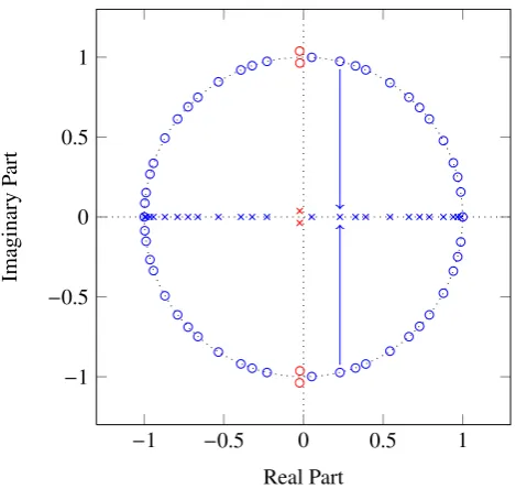
Fig. 5.Roots of a typical polynomial
In Fig. 5 the zeros of the polynomial belonging to the
beampattern (according to Eq. (3)) of the array with
p
=
(0 0
.
1 0
.
2 0
.
3 1
.
4 1
.
5 2
.
6 2
.
7)
Tare shown. Both the basic
algorithm described in Sect. 4 and the improved algorithm
from Sect. 5 are depicted in the figure. The zeros of the
ba-sic algorithm are drawn as circles. The red roots have to be
discarded due to the rooting constraint. The crosses are the
roots of the optimized algorithm. Again, the roots which do
not satisfy the constraint are shown in red. Every complex
conjugate pair of the circular roots from the basic algorithm
results in one root from the improved algorithm as a
projec-tion on the real axis.
A comparison between a sampling algorithm and a rooting
algorithm strongly depends on the used algorithms.
Never-theless some general facts can be stated.
–
The order of the polynomial, which must be rooted, is
given by 2
pN−1gcd(p)
with the general algorithm. The
opti-mized algorithm leads to an order of
pN−1 gcd(p)−
1.
–
As the rooting is the dominant part, the algorithm is
in-dependent of the number of sensors for constant gcd(
p
).
–
Keeping the gcd constant, the polynomial scales linearly
with the aperture.
–
Scaling the whole array does not change the algorithm’s
e
ffi
ciency.
–
The algorithm is slow if the sensor positions are nearly
relatively prime. As manufacturing tolerances limit the
positional precision, only allowing positions on a grid
with a grid size in the magnitude of the production
tol-erances does not add an additional constraint.
–
Most of the roots of the polynomials satisfy the
con-straints and lead to extrema, as seen in Fig. 5.
Antenna positions Order Reduced Order
0, 0.5, 1.5 6 2
0, 0.4, 1.5 30 14
0, 1.3, 2.05 82 40
0, 0.4, 1.7, 4.3 86 42
0, 0.1, 0.2, 0.3, 1.4, 1.5, 2.6, 2.7 54 26 0, 0.78, 2.44, 5.32 532 –
Table 1. Polynomial orders of arrays for general and improved al-gorithm
–
The calculation of the binomial coe
ffi
cients in Eq. (9)
can be time consuming for larger polynomial orders,
re-ducing the rooting time benefits. Precalculating the
bi-nomials and saving them into a lookup table avoids this
additional e
ff
ort. Nevertheless for very large
polyno-mial orders (
>
50), some binomial coe
ffi
cients get too
large resulting in numerical problems. This can be seen
in Fig. 5 as well, as the roots at about 1 and
−
1 get very
close due to the negligence of the imaginary part.
Some examples of sensor positions and polynomial orders
are given in Table 1. The order of the last array for the
im-proved algorithm is not given, as only the base algorithm can
be used due to the aforementioned numerical problems.
In Fig. 6 we compare the evaluation time of a sampling and
the basic rooting algorithm. The sampling algorithm
sam-ples with a spatial frequency slightly higher than Nyquist’s
frequency and performs a local maximization starting at
ev-ery sample. The sampling algorithm does not always find all
maxima as shown in Fig. 4. We defined two parametrized
ar-ray positions depending on
o
. The positions of both
param-eterizations get more and more “prime” with increasing
o
.
The first parametrization uses a fixed aperture
p
=
0 (
o+111)
T,
which is the best case (bc) for the sampling algorithm. The
second one is a dynamic aperture
p
=
(0 0
.
5 0
.
5(
o
+
1))
T,
be-ing some sort of worst case (wc) parametrization regardbe-ing
the sampling.
We see, that the sampling algorithm runs approximately
in constant time having a constant aperture, i.e. constant
Nyquist frequency Eq. (4). With the growing aperture
re-alization the sampling algorithm is slow even for relatively
small
o
. These two lines are the lower and upper limit of
the sampling performance, so that most arrays will have a
sampling performance in the area between both lines.
The rooting algorithm executes very fast for normal arrays.
The unsteady behavior from
o
=
36 to
o
=
37 is a reproducible
problem of Matlab’s rooting algorithm. The rooting
algo-rithm scales as before independent of the aperture increase.
If the gcd is very small compared to the aperture, the rooting
algorithm is slower than the sampling algorithm. For most
practically important arrays (small
o
), the new algorithm is
between one and two magnitudes faster than the sampling
algorithm.
Fig. 5. Roots of a typical polynomial.
6 Results
It’s interesting to note, that due to the various differences in Eqs. (3) and (4), coefficients can have components from more than one position in Eq. (5). An example would be a ULA (Uniform Linear Array). On the other hand, MRAs (Mof-fet, 1968) (Minimum Redundancy Array) consisting of opti-mum Golomb rulers (Tavares et al., 2005) have no frequency twice. So the multiplicity of frequencies is a measure of the redundancy of the array.
In Fig. 5 the zeros of the polynomial belonging to the beampattern – according to Eq. (3) – of the array withp= (0 0.1 0.2 0.3 1.4 1.5 2.6 2.7)Tare shown. Both the basic algorithm described in Sect. 4 and the improved algorithm from Sect. 5 are depicted in the figure. The zeros of the ba-sic algorithm are drawn as circles. The red roots have to be discarded due to the rooting constraint. The crosses are the roots of the optimized algorithm. Again, the roots which do not satisfy the constraint are shown in red. Every complex conjugate pair of the circular roots from the basic algorithm results in one root from the improved algorithm as a projec-tion on the real axis.
A comparison between a sampling algorithm and a rooting algorithm strongly depends on the used algorithms. Never-theless some general facts can be stated.
– The order of the polynomial, which must be rooted, is given by 2pN−1
gcd(p) with the general algorithm. The
opti-mized algorithm leads to an order of pN−1
gcd(p)−1.
– As the rooting is the dominant part, the algorithm is in-dependent of the number of sensors for constant gcd(p).
Table 1. Polynomial orders of arrays for general and improved
al-gorithm.
Antenna positions Order Reduced Order
0, 0.5, 1.5 6 2
0, 0.4, 1.5 30 14
0, 1.3, 2.05 82 40
0, 0.4, 1.7, 4.3 86 42
0, 0.1, 0.2, 0.3, 1.4, 1.5, 2.6, 2.7 54 26
0, 0.78, 2.44, 5.32 532 –
– Keeping the gcd constant, the polynomial scales linearly with the aperture.
– Scaling the whole array does not change the algorithm’s efficiency.
– The algorithm is slow if the sensor positions are nearly relatively prime. As manufacturing tolerances limit the positional precision, only allowing positions on a grid with a grid size in the magnitude of the production tol-erances does not add an additional constraint.
– Most of the roots of the polynomials satisfy the con-straints and lead to extrema, as seen in Fig. 5.
– The calculation of the binomial coefficients in Eq. (9) can be time consuming for larger polynomial orders, re-ducing the rooting time benefits. Precalculating the bi-nomials and saving them into a lookup table avoids this additional effort. Nevertheless for very large polyno-mial orders (>50), some binomial coefficients get too large resulting in numerical problems. This can be seen in Fig. 5 as well, as the roots at about 1 and−1 get very close due to the negligence of the imaginary part. Some examples of sensor positions and polynomial orders are given in Table 1. The order of the last array for the im-proved algorithm is not given, as only the base algorithm can be used due to the aforementioned numerical problems.
In Fig. 6 we compare the evaluation time of a sampling and the basic rooting algorithm. The sampling algorithm sam-ples with a spatial frequency slightly higher than Nyquist’s frequency and performs a local maximization starting at ev-ery sample. The sampling algorithm does not always find all maxima as shown in Fig. 4. We defined two parametrized ar-ray positions depending ono. The positions of both parame-terizations get more and more “prime” with increasingo. The first parametrization uses a fixed aperturep=0 (o+11 1)T, which is the best case (bc) for the sampling algorithm. The second one is a dynamic aperturep=(0 0.5 0.5(o+1))T, being some sort of worst case (wc) parametrization regard-ing the samplregard-ing.
P. H¨acker et al.: Fast beampattern evaluation by polynomial rooting 151
:
7
10 30 50 70 90 110 130 10−3
10−2 10−1 100
o
Time
in
s
pwc,sampling
pbc,sampling
pwc,rooting
pbc,rooting
Fig. 6. Evaluation time comparison between sampling and rooting algorithm
0.5 0.6 0.7 0.8 0.9 1 0
0.2 0.4 0.6 0.8 1
Maximum side lobe height Cumulative distribution function
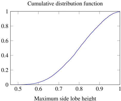
Fig. 7.Maximum side lobe height distribution of 156 849 calculated beampatterns
To show the new possibilities with the described
algo-rithm, we performed a systematic search for arrays with a
minimum maximum similarity in the whole angular range.
Therefore we used an array with 5 elements and an
aper-ture of ten wavelengths. Note, that this is nearly twice the
aperture of an optimum MRA with 5 elements and violates
Nyquist by a factor of five, so the array will be extremly
sparse and most of the possible arrays’ beampattern have
very huge side lobes. The grid size of the systematic search
was 0
.
1
◦which lead to the calculation of
993=
156849
beam-patterns. The minimum maximum similarity is 0
.
462 for the
array positions (0 1
.
6 4
.
8 6 10)
T. Only 0
.
063% of all
calcu-lated beampatterns have a side lobe maximum lower than 0
.
5.
The empirical cumulative distribution function of all
maxi-mum side lobe heights is shown in Fig. 7.
7
Conclusions
We proposed an algorithm finding all maxima of a
beampat-tern. Therefore the antenna positions have to be on a grid,
which can always be approximated with arbitrary precision.
The algorithm formulates the problem as a polynomial via a
generalized version of gcd and locates the maxima by
root-ing the derivative. The algorithm accelerates sensor array
optimization. We suggested an extension to the algorithm,
which reduces the time for low and medium polynomial
or-ders even more. We showed the successful application of
the algorithm by finding an array with a very good
aperture-to-side-lobe-height ratio. Further work should investigate if
a similar algorithm can be found for combined azimuth and
elevation estimation.
8
Acknowledgement
This research has been conducted in cooperation with the
Robert Bosch Corporation, to which the authors would like
to express their gratitude.
References
Athley, F.: Threshold Region Performance of Maximum Likelihood Direction of Arrival Estimators, IEEE Trans. on Signal Process-ing, 53, 2005.
Athley, F., Engdahl, C., and Sunnergren, P.: Model-based Detection and Direction of Arrival Estimation in RADAR using Sparse Ar-rays, vol. 2, doi:10.1109/ACSSC.2004.1399505, 2004.
Bronshtein, I. N., Musiol, G., M¨uhlig, H., and Semendyayev, K. A.: Handbook of Mathematics, Springer, 4th edn., 2004.
Cormen, T. H., Leiserson, C. E., Rivest, R. L., and Stein, C.: In-troduction to Algorithms, MIT Press and McGraw-Hill, 2 edn., 2001.
Jurgen, R. K.: Adaptive Cruise Control, SAE International, 2006. Moffet, A.: Minimum-Redundancy Linear Arrays, IEEE Trans. on
Antennas and Propagation, 16, 1968.
Rockett, A. M. and Sz¨usz, P.: Continued Fractions, World Scien-tific, 2 edn., 1992.
Rosen, K. H. and Michaels, J. G.: Handbook of discrete and com-binatorial mathematics, CRC Press, 3 edn., 2000.
Ruder, M., Enkelmann, W., and Garnitz, R.: Highway Lane Change Assistant, in: IEEE Intelligent Vehicle Symposium, vol. 1, doi: 10.1109/IVS.2002.1187958, 2002.
Tavares, J., Leit˜ao, T., Pereira, F. B., and Costa, E.: Evolving Seg-ments Length in Golomb Rulers, in: Adaptive and Natural Com-puting Algorithms, Proc. International Converence in Coimbra, doi:10.1007/3-211-27389-1 57, 2005.
Fig. 6. Evaluation time comparison between sampling and rooting
algorithm.
We see, that the sampling algorithm runs approximately in constant time having a constant aperture, i.e. constant Nyquist frequency Eq. (4). With the growing aperture re-alization the sampling algorithm is slow even for relatively small o. These two lines are the lower and upper limit of the sampling performance, so that most arrays will have a sampling performance in the area between both lines.
The rooting algorithm executes very fast for normal ar-rays. The unsteady behavior fromo=36 too=37 is a re-producible problem of Matlab’s rooting algorithm. The root-ing algorithm scales as before independent of the aperture increase. If the gcd is very small compared to the aperture, the rooting algorithm is slower than the sampling algorithm. For most practically important arrays (smallo), the new al-gorithm is between one and two magnitudes faster than the sampling algorithm.
To show the new possibilities with the described algo-rithm, we performed a systematic search for arrays with a minimum maximum similarity in the whole angular range. Therefore we used an array with 5 elements and an aper-ture of ten wavelengths. Note, that this is nearly twice the aperture of an optimum MRA with 5 elements and violates Nyquist by a factor of five, so the array will be extremly sparse and most of the possible arrays’ beampattern have very huge side lobes. The grid size of the systematic search was 0.1◦ which lead to the calculation of 993=156849 beampatterns. The minimum maximum similarity is 0.462 for the array positions(0 1.6 4.8 6 10)T. Only 0.063% of all calculated beampatterns have a side lobe maximum lower than 0.5. The empirical cumulative distribution function of all maximum side lobe heights is shown in Fig. 7.
:
7
10
30
50
70
90
110
130
10
−310
−210
−110
0o
Time
in
s
p
wc,samplingp
bc,samplingp
wc,rootingp
bc,rootingFig. 6.
Evaluation time comparison between sampling and rooting
algorithm
0
.
5
0
.
6
0
.
7
0
.
8
0
.
9
1
0
0
.
2
0
.
4
0
.
6
0
.
8
1
Maximum side lobe height
Cumulative distribution function
Fig. 7.
Maximum side lobe height distribution of 156 849 calculated
beampatterns
To show the new possibilities with the described
algo-rithm, we performed a systematic search for arrays with a
minimum maximum similarity in the whole angular range.
Therefore we used an array with 5 elements and an
aper-ture of ten wavelengths. Note, that this is nearly twice the
aperture of an optimum MRA with 5 elements and violates
Nyquist by a factor of five, so the array will be extremly
sparse and most of the possible arrays’ beampattern have
very huge side lobes. The grid size of the systematic search
was 0
.
1
◦which lead to the calculation of
993=
156849
beam-patterns. The minimum maximum similarity is 0
.
462 for the
array positions (0 1
.
6 4
.
8 6 10)
T. Only 0
.
063% of all
calcu-lated beampatterns have a side lobe maximum lower than 0
.
5.
The empirical cumulative distribution function of all
maxi-mum side lobe heights is shown in Fig. 7.
7
Conclusions
We proposed an algorithm finding all maxima of a
beampat-tern. Therefore the antenna positions have to be on a grid,
which can always be approximated with arbitrary precision.
The algorithm formulates the problem as a polynomial via a
generalized version of gcd and locates the maxima by
root-ing the derivative. The algorithm accelerates sensor array
optimization. We suggested an extension to the algorithm,
which reduces the time for low and medium polynomial
or-ders even more. We showed the successful application of
the algorithm by finding an array with a very good
aperture-to-side-lobe-height ratio. Further work should investigate if
a similar algorithm can be found for combined azimuth and
elevation estimation.
8
Acknowledgement
This research has been conducted in cooperation with the
Robert Bosch Corporation, to which the authors would like
to express their gratitude.
References
Athley, F.: Threshold Region Performance of Maximum Likelihood
Direction of Arrival Estimators, IEEE Trans. on Signal
Process-ing, 53, 2005.
Athley, F., Engdahl, C., and Sunnergren, P.: Model-based Detection
and Direction of Arrival Estimation in RADAR using Sparse
Ar-rays, vol. 2, doi:10.1109
/
ACSSC.2004.1399505, 2004.
Bronshtein, I. N., Musiol, G., M¨uhlig, H., and Semendyayev, K. A.:
Handbook of Mathematics, Springer, 4th edn., 2004.
Cormen, T. H., Leiserson, C. E., Rivest, R. L., and Stein, C.:
In-troduction to Algorithms, MIT Press and McGraw-Hill, 2 edn.,
2001.
Jurgen, R. K.: Adaptive Cruise Control, SAE International, 2006.
Mo
ff
et, A.: Minimum-Redundancy Linear Arrays, IEEE Trans. on
Antennas and Propagation, 16, 1968.
Rockett, A. M. and Sz¨usz, P.: Continued Fractions, World
Scien-tific, 2 edn., 1992.
Rosen, K. H. and Michaels, J. G.: Handbook of discrete and
com-binatorial mathematics, CRC Press, 3 edn., 2000.
Ruder, M., Enkelmann, W., and Garnitz, R.: Highway Lane Change
Assistant, in: IEEE Intelligent Vehicle Symposium, vol. 1, doi:
10.1109
/
IVS.2002.1187958, 2002.
Tavares, J., Leit˜ao, T., Pereira, F. B., and Costa, E.: Evolving
Seg-ments Length in Golomb Rulers, in: Adaptive and Natural
Com-puting Algorithms, Proc. International Converence in Coimbra,
doi:10.1007
/
3-211-27389-1 57, 2005.
Fig. 7. Maximum side lobe height distribution of 156 849 calculated
beampatterns.
7 Conclusions
We proposed an algorithm finding all maxima of a beampat-tern. Therefore the antenna positions have to be on a grid, which can always be approximated with arbitrary precision. The algorithm formulates the problem as a polynomial via a generalized version of gcd and locates the maxima by root-ing the derivative. The algorithm accelerates sensor array optimization. We suggested an extension to the algorithm, which reduces the time for low and medium polynomial or-ders even more. We showed the successful application of the algorithm by finding an array with a very good aperture-to-side-lobe-height ratio. Further work should investigate if a similar algorithm can be found for combined azimuth and elevation estimation.
Acknowledgements. This research has been conducted in
coopera-tion with the Robert Bosch Corporacoopera-tion, to which the authors would like to express their gratitude.
References
Athley, F.: Threshold Region Performance of Maximum Likelihood Direction of Arrival Estimators, IEEE Trans. on Signal Process-ing, 53, 1359–1373, 2005.
Athley, F., Engdahl, C., and Sunnergren, P.: Model-based Detection and Direction of Arrival Estimation in RADAR using Sparse Ar-rays, 2, 1953–1957, doi:10.1109/ACSSC.2004.1399505, 2004. Bronshtein, I. N., Musiol, G., Mhlig, H., and Semendyayev, K. A.:
Handbook of Mathematics, Springer, 4th edn., 2004.
Cormen, T. H., Leiserson, C. E., Rivest, R. L., and Stein, C.: In-troduction to Algorithms, MIT Press and McGraw-Hill, 2 edn., 2001.
152 P. H¨acker et al.: Fast beampattern evaluation by polynomial rooting
Jurgen, R. K.: Adaptive Cruise Control, SAE International, 2006. Moffet, A.: Minimum-Redundancy Linear Arrays, IEEE Trans. on
Antennas and Propagation, 16, 172–175, 1968.
Rockett, A. M. and Szsz, P.: Continued Fractions, World Scientific, 2 edn., 1992.
Rosen, K. H. and Michaels, J. G.: Handbook of discrete and com-binatorial mathematics, CRC Press, 3 edn., 2000.
Ruder, M., Enkelmann, W., and Garnitz, R.: Highway Lane Change Assistant, in: IEEE Intelligent Vehicle Symposium, 1, 240–244, doi:10.1109/IVS.2002.1187958, 2002.
Tavares, J., Leito, T., Pereira, F. B., and Costa, E.: Evolving Seg-ments Length in Golomb Rulers, in: Adaptive and Natural Com-puting Algorithms, Proc. International Converence in Coimbra, 239–242, doi:10.1007/3-211-27389-1 57, 2005.