Fixed Point Theory and Applications Volume 2011, Article ID 615274,17pages doi:10.1155/2011/615274
Research Article
Hamming Star-Convexity Packing in
Information Storage
Mau-Hsiang Shih and Feng-Sheng Tsai
Department of Mathematics, National Taiwan Normal University, 88 Section 4, Ting Chou Road, Taipei 11677, Taiwan
Correspondence should be addressed to Feng-Sheng Tsai,[email protected]
Received 8 December 2010; Accepted 16 December 2010
Academic Editor: Jen Chih Yao
Copyrightq2011 M.-H. Shih and F.-S. Tsai. This is an open access article distributed under the Creative Commons Attribution License, which permits unrestricted use, distribution, and reproduction in any medium, provided the original work is properly cited.
A major puzzle in neural networks is understanding the information encoding principles that implement the functions of the brain systems. Population coding in neurons and plastic changes in synapses are two important subjects in attempts to explore such principles. This forms the basis of modern theory of neuroscience concerning self-organization and associative memory. Here we wish to suggest an information storage scheme based on the dynamics of evolutionary neural networks, essentially reflecting the meta-complication of the dynamical changes of neurons as well as plastic changes of synapses. The information storage scheme may lead to the development of a complete description of all the equilibrium statesfixed pointsof Hopfield networks, a space-filling network that weaves the intricate structure of Hamming star-convexity, and a plasticity regime that encodes information based on algorithmic Hebbian synaptic plasticity.
1. Introduction
The study of memory includes two important components: the storage component of memory and the systems component of memory1,2. The first is concerned with exploring
the molecular mechanisms whereby memory is stored, whereas the second is concerned with analyzing the organizing principles that mediate brain systems to encode, store, and retrieve memory. The first neurophysiological description about the systems component of
memory was proposed by Hebb 3. His postulate reveals a principle of learning, which
is often summarized as “the connections between neurons are strengthened when they fire simultaneously.” The Hebbian concept stimulates an intensive effort to promote the building of associative memory models of the brain 4–9. Also, it leads to the development of a
an Ising model used in statistical physics12–15, and the study of constrained optimization
problems such as the famous traveling salesman problem16.
However, since it was initiated by Kohonen and Anderson in 1972, associative memory has remained widely open in neural networks 17–21. It generally includes questions
concerning a description of collective dynamics and computing with attractors in neural networks. Hence the central question22: “given an arbitrary set of prototypes of 01-strings
of length n, is there any recurrent network such that the set of all equilibrium states of this network is exactly the set of those prototypes?” Many attempts have been made to tackle this problem. For instance, using the method of energy minimization, Hopfield in 1982 constructed a network of nerve cells whose dynamics tend toward an equilibrium state when the retrieval operation is performed asynchronously13. Furthermore, to circumvent limited
capacity in storage and retrieval of Hopfield networks, Personnaz et al. in 1986 investigated the behavior of neural networks designed with the projection rule, which guarantees the errorless storage and retrieval of prototypes23,24. In 1987, Diederich and Opper proposed
an iterative scheme to substitute a local learning rule for the projection rule when the prototypes are linearly independent25,26. This sheds light on the possibility of storing
correlated prototypes in neural networks with local learning rules.
In addition to the discussion on learning mechanisms for associative memory, Hopfield networks have also given a valuable impetus to basic research in combinatorial fixed point theory in neural networks. In 1992, Shrivastava et al. conducted a convergence analysis of a class of Hopfield networks and showed that all equilibrium states of these networks have a one-to-one correspondence with the maximal independent sets of certain undirected graphs 27. M ¨uezzino ˘glu and G ¨uzelis¸ in 2004 gave a further compatibility
condition on the correspondence between equilibrium states and maximal independent sets, which avoids spurious stored patterns in information storage and provides attractiveness of prototypes in retrieval operation28. Moreover, the analytic approach of Shih and Ho29
in 1999 as well as Shih and Dong30in 2005 illustrated the reverberating-circuit structure to determine equilibrium states in generalized boolean networks, leading to a solution of the boolean Markus-Yamabe problem and a proof of network perspective of the Jacobian conjecture, respectively.
More recently, we described an evolutionary neural network in which the connection strengths between neurons are highly evolved according to algorithmic Hebbian synaptic plasticity 31. To explore the influence of synaptic plasticity on the evolutionary neural
network’s dynamics, a sort of driving forces from the meta-complication of the evolutionary neural network’s nodal-and-coupling activities is introduced, in contrast with the explicit construction of global Lyapunov functions in neural networks 10, 13, 32, 33 and in accordance with the limitation of finding a common quadratic Lyapunov function to control a switched system’s dynamics34–36. A mathematical proof asserts that the ongoing changes
of the evolutionary network’s nodal-and-coupling dynamics will eventually come to rest at equilibrium states31. This result reflects, in a deep mathematical sense, that plastic changes
in the coupling dynamics may appear as a mechanism for associative memory.
a plasticity regime that guides the evolution of the primitive neural network such that each vertex in the merging domain will tend toward the unique prototype underlying the dynamics of the resulting evolutionary neural network.
Our point of departure is the convexity packing lurking behind Hopfield networks. We consider the domain of attraction in which every initial state in the domain tends toward the equilibrium state asynchronously. For the asynchronous operating mode, each trajectory in the phase space can represent as one of the “connected” paths between the initial state and the equilibrium state when it is measured by the Hamming metric. It provides a clear map that all the domains of attraction in Hopfield networks are star-convexity-like and that the phase space can be filled with those star-convexity-like domains. And it applies to frame a primitive Hopfield network that might consolidate an insight of exploring a plasticity regime in the information storage scheme.
2. Information Storage of Hopfield Networks
Let{0,1}n denote the binary code consisting of all 01 strings of fixed lengthn, and letX
{x1, x2, . . . , xp} be an arbitrary set of prototypes in {0,1}n. For each positive integer
k, let
Æk {1,2, . . . , k}. Using the formal neurons of McCulloch and Pitts37, we can construct
a Hopfield network of ncoupled neurons, namely, 1,2, . . . , n, whose synaptic strengthsare listed in an array, denoted by the matrixA aijn×n, and defined on the basis of the Hebbian learning rule, that is,
aij p
s1
xsixsj for everyi, j∈Æn. 2.1
Thefiring stateof each neuroniis denoted byxi 1, whereas the quiescent stateisxi 0.
The function is the Heaviside function: u 1 foru≥ 0, otherwise 0, which describes an instantaneous unit pulse. The dynamics of the Hopfield network is encoded by the function
F f1, f2, . . . , fn, where
fix
⎛ ⎝n
j1
aijxj−bi ⎞
⎠ 2.2
encodes the dynamics of neuroni,x x1, x2, . . . , xnis a vector ofstate variablesin the phase
space{0,1}n, andbi∈Êis thethresholdof neuronifor eachi∈Æn.
For everyx, y∈ {0,1}n, define the vectorial distancebetweenxandy38,39, denoted
asdx, y, to be
dx, y
⎛ ⎜ ⎜ ⎜ ⎝
x1−y1 .. . xn−yn
⎞ ⎟ ⎟ ⎟
For everyx, y ∈ {0,1}n, define the order relationx≤ ybyxi ≤yi for eachi∈Æn; thechain
intervalbetweenxandy, denoted asCx, y, to be
Cx, yz∈ {0,1}n;dz, y≤dx, y. 2.4
Note thatCx, y Cy, x, and the notationCx, ymeans thatCx, y\ {x}. TheHamming
metricρHon{0,1}nis defined to be
ρH
x, y#i∈Æn;xi/yi
2.5
for everyx, y ∈ {0,1}n 40. Denote byγx, y a chain joiningx andy with the minimum
Hamming distance, meaning that
γx, yx, u1, u2, . . . , ur−1, y, 2.6
whereρHui, ui1 1 fori0,1, . . . , r−1 withu0 x, ur y, andρHx, u1 ρHu1, u2
· · ·ρHur−1, y ρHx, y. Then we haveCx, y γx, y, where the union is taken over
all chains joiningxandywith the minimum Hamming distance. Denote by·,· the Euclidean scalar product in Ê
n. A set of elementsyα in{0,1}n,
whereαruns through some index set inI, is calledorthogonalifyα, yβ0 for eachα, β∈I with α /β. Two sets Y andZ in{0,1}n are calledmutually orthogonalify, z 0 for each
y ∈ Y andz ∈ Z. Given a set Y {y1, y2, . . . , yq} in{0,1}n, we define the 01-spanofY, denoted as 01-spanY, to be the set consists of all elements of the formτ1y1τ2y2· · ·τqyq, whereτi∈ {0,1} for eachi∈Æq. We assume thatx
i
/
0 for eachi∈Æp. For eachi∈Æp, define
Nx1i
xs∈X;xs, xi/0 2.7
and define recursively
Nxj1i
xs∈X;
xs, xk
/
0 for some xk∈Æ
j xi
2.8
for eachj ∈Æ. Clearly, for eachi∈Æpwe have
Nx1i ⊂N2xi ⊂Nx3i ⊂ · · · , 2.9
and thereby there exists a smallest positive integer, denoted assi, such that
NxsiiN
sij
xi for eachj ∈Æ. 2.10
It is readily seen that for eachi∈Æpand for eachx
j∈Nsi
xi , we have
NxsiiN
sj
and clearly, for everyi, j ∈Æp, exactly one of the following conditions holds:
NxsiiN
sj
xj or N
si xi ∩N
sj
xj ∅. 2.12
According to 2.8 and 2.12, we can pick all distinct sets N1, N2, . . . , Nq from {Nxs11 ,
Nxs22 , . . . , N sp
xp }and obtain theorthogonal partitionofX, that is,NiandNjare mutually or-thogonal for everyi /j andXi∈qNi. For eachk∈
Æq, define
ξk
⎛ ⎜ ⎜ ⎜ ⎝
maxx1i;xi∈N k
.. .
maxxi
n;xi∈Nk
⎞ ⎟ ⎟ ⎟
⎠. 2.13
Then we have the orthogonal set{ξ1, ξ2, . . . , ξq}generated by the orthogonal partition ofX, which is denoted as GopX.
Using the “orthogonal partition,” we can give a complete description of the equi-librium states of the Hopfield network encoded by 2.1 and 2.2 with ultra-low thresh-olds.
Theorem 2.1. LetXbe a set consisting of nonzero vectors in{0,1}n, and let the functionFbe defined by2.1and2.2with0< bi ≤1for eachi∈Æn. Then,FixF 01-spanGopX.
Proof. LetX {x1, x2, . . . , xp}and let GopX {ξ1, ξ2, . . . , ξq}. By orthogonality of GopX,
1−qi1ξi
jis 0 or 1 for eachj∈Æn. Thus the pointÁGopX, defined by
Á
GopX
1−
q
i1
ξi1,1− q
i1
ξ2i, . . . ,1− q
i1
ξin
, 2.14
lies in{0,1}n. LetU0 C0,ÁGopXandUi C0, ξ
ifor eachi∈
Æq. Note that the sets
UiandUjare mutually orthogonal for everyi /j. Letξ q
i1αiξiforαi ∈ {0,1}andi∈Æq.
We prove now thatFξ ξby showing that
Fx∈Cx, ξ for eachx∈U0
q
i1
αiUi. 2.15
we have
Fx
⎛ ⎝p
i1
xiTu0xi
q j1 p i1 αj
xiTujxi−b
⎞ ⎠
⎛ ⎝q
j1
xi∈N j
αj
xiTujxi−b
⎞ ⎠
≤q j1
αjξj.
2.16
Thus we need only consider the caseFxν 0 andξν 1 for someν∈Æn. Under the case,
there existsr∈Æq such thatαr 1 andξ
r
ν1, so that
Fxν≥ ⎛
⎝
xi∈N r
xiTurxiν−bν ⎞ ⎠
≥ ⎛
⎝
xi∈N r
urν
xνi 2
−bν ⎞ ⎠.
2.17
Since Fxν 0, we have xν urν 0. This implies that dFx, ξ ≤ dx, ξ, that is,
Fx∈Cx, ξ.
We turn now to prove thatFx/xfor eachx /∈01-spanGopX. To accomplish this,
we first show that
{0,1}n
αi∈{0,1}, i∈
q
U0
q
i1
αiUi. 2.18
Letx∈ {0,1}n. We associate to eachi∈Æq a point
zix1ξi1, x2ξi2, . . . , xnξin
2.19
and putz0x−q
i1zi. Then for eachi∈Æq, there existαi ∈ {0,1}such thatz
i∈α
iUi. Since for eachk∈Æn
z0kxk− q
i1
xkξki ≤1− q
i1
ξik, 2.20
we have z0 ∈ U
0, proving 2.18. Thus each x /∈01-spanGopX can be written as
x u0q
i1αiui, whereαi ∈ {0,1},ui ∈Ui fori 0,1, . . . , qand, further, we have either
u0/0 or there existsr∈Æq such thatαr 1 andu
r
/
Case 1u0
/
0. Then there existsν ∈ Æn such thatu
0
ν 1 andxkν 0 for eachk ∈Æp. This
implies that
xνu0ν q
i1
αiuiν1,
Fxν ⎛ ⎝q
j1
xi∈N j
αj
xiTujxiν
−bν ⎞ ⎠0,
2.21
provingFx/x.
Case 2. There existsr∈Æq such thatαr 1 andu
r
/
ξr. Then
C0, ξr∩X\C0, ur∩X\C0, ξr−ur/∅. 2.22
Indeed, if the left hand side of2.22is empty, then for everyxi ∈Nr X∩C0, ξr, exactly one of the following conditions holds:
xi∈C0, ur or xi∈C0, ξr−ur. 2.23
Divide the setNr into two subsets:
xi∈M1 if xi ∈C0, ur,
xi∈M2 if xi ∈C0, ξr−ur.
2.24
Then, by the construction ofξr, we haveM
1/∅andM2/∅. Now letxσ ∈M1 andxη ∈M2.
Since M1 and M2 are mutually orthogonal, we get Nxsσσ ⊂ M1 and Nxsηη ⊂ M2. This
con-tradicts
NxsσσN
sη
xη Nr, 2.25
proving2.22. Therefore, there exist
xk∈C0, ξr∩X\C0, ur∩X\C0, ξr−ur 2.26
andk1, k2 ∈Æn withu
r
k1 1 andξ r−ur
k2 1 such thatx k k1 x
k
k2 1. Sinceξ r−ur
uik2 0 fori0,1, . . . , qandxki2 0 for eachxi/∈N
r. This implies that
xk2 u
0
k2 q
i1
αiuik20,
Fxk2 ≥
⎛
⎝
xi∈N r
xiTurxik2−bk2
⎞ ⎠
≥ xk k1u
r k1x
k k2−bk2
1,
2.27
revealingFx/x, provingTheorem 2.1.
3. Domains of Attraction and Hamming Star-Convex Building Blocks
By analogy with the notion of star-convexity in vector spaces, a setUin{0,1}nis said to be
Hamming star-convexif there exists a pointy ∈Usuch thatCx, y ⊂Ufor eachx ∈U. We
callya star-centerofU.
LetX be a set in{0,1}n, and letΛX denote the collection of all 01-spanY, whereY
is an orthogonal set consisting of nonzero vectors in{0,1}n, such thatX ⊂01-spanY. Then
ΛX/∅. Indeed, if the order “≤” onΛXis defined byA≤Bif and only ifA⊂B, thenΛX,≤
becomes a partially ordered set and there exists an orthogonal setY such that 01-spanYis minimal inΛX. We call suchYthekernelofX. A labeling procedure for establishing the kernel
Y ofX is described as follows. LetX {x1, x2, . . . , xp}in{0,1}n. If
X {0}, thenY {y},
wherey /0, is the kernel ofX. Otherwise, define the labelings
λi
x1i, x2i, . . . , x p i
for eachi∈Æn 3.1
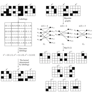
and pick all distinct nonzero labelingsv1, v2, . . . , vq fromλ1, λ2, . . . , λn. Then the orthogonal set Y {y1, y2, . . . , yq}, given byyji 1 if λj vi, otherwise yij 0 for eachi ∈ Æq and
j ∈Æn, is the kernel ofXseeFigure 1. Note that since the computation of the kernel can be
implemented by radix sort, its computational complexity is inΘpn.
LetY {y1, y2, . . . , yq} be the kernel ofX. We associate to eachyk ∈ Y an integer
nk∈Æ, two sets of nodes
Vk
vk,l; l∈Ænk
, Wk
wk,j; ykj 1, j∈Æn
, 3.2
and a set of edgesEksuch thatGk Vk∪Wk, Ekis a simple, connected, and bipartite graph with color classesVkand Wk.The graph-theoretic notion and terminologies can be found in 41. For eachj ∈ Æn, put u
k,l
j 1 if vk,l and wk,j are adjacent, otherwise 0. LetG {G1, G2, . . . , Gq}and denote by BipY, Gthe collection of all vectorsuk,l constructed by the
n(1) =4 n(2) =2 n(3) =3 Bipartite
graphs
v1,1 v1,2 v1,3 v1,4
v3,1 v3,2 v3,3 v2,1
v2,2 w1,1 w1,3 w1,8 w1,9 w1,12
w2,4 w2,7 w2,15 w2,16
w3,10 w3,11 w3,13
x1 x2 x3
(1, 0, 0) (0, 0, 0)
(0, 0, 0) (0, 0, 0)
(0, 0, 0)
(1, 1, 0)
(1, 1, 0) (1, 1, 0)
(1, 1, 0) (0, 1, 1)
(0, 1, 1) (1, 0, 0) (1, 0, 0)
(0, 1, 1)
(0, 1, 1)
(0, 1, 1)
y1 y2 y3
G1 G2 G3
u1,1 u1,2 u1,3 u1,4
u2,1 u2,2
u3,1 u3,2 u3,3
Bip(Y, G)
y1 y2 y3
v1= (0,1,1),v2= (1,1,0),v3= (1,0,0)
The kernel determined by labelings Labelings
Non-zero labelings
Figure 1:A schematic illustration of the generation of the kernelYand BipY, G.
Denote by FixFthe set of all equilibrium statesfixed points ofF and denote by
DGSξthe domain of attraction of the equilibrium stateξunderlying Gauss-Seidel iteration
a particular mode of asynchronous iteration
xit1 fix1t1, . . . , xi−1t1, xit, . . . , xnt 3.3
fort0,1, . . .andi∈Æn.
Theorem 3.1. LetXbe a subset of{0,1}n, and letY {y1, y2, . . . , yq}be the kernel ofX. Associate to each
BipY, G uk,l; k∈Æq, l∈Ænk
a functionFdefined by2.2with
aij q
k1
nk
l1
uk,li uk,lj for eachi, j∈Æn 3.5
and0< bi≤1for eachi∈Æn. Then
iX ⊂FixF;
iifor eachξ ∈FixF, the domain of attractionDGSξis Hamming star-convex withξas a
star-center.
Proof. For eachk∈Æq, sinceGkis simple, connected, and bipartite with color classesVkand
Wk, we have
Nusk,lk,lN
sk,j
uk,j for eachl, j∈Ænk. 3.6
It follows from the orthogonality ofY that
uk,l; l∈Ænk
⊂Nusk,jk,j⊂C
0, yk 3.7
for eachk∈Æq andj∈Ænk. Furthermore, sinceGkis connected for eachk∈Æq, we have
maxuk,lj ; l∈Ænk
yk
j for eachj∈Æn. 3.8
This implies that GopBipY, G Y, and byTheorem 2.1, we have
FixF 01-spanGopBipY, G⊃X, 3.9
provingi. To proveii, we first show that for eachi∈Æq andαi∈ {0,1},
C0,ÁY
q
i1
αiC
0, yi⊂DGS
q
i1
αiyi
, 3.10
whereÁY 1−
q
i1yi1,1− q
i1yi2, . . . ,1− q
i1yin. LetUdenote the set in the left hand side of3.10, and letx∈U,yqi1αiyi, andz∈Cx, y. Splitzinto two parts:
z
z1−
q
i1
z1yi1, z2−
q
i1
z2yi2, . . . , zn− q
i1
znyin
q
i1
z1y1i, z2yi2, . . . , znyin
. 3.11
Then the first part ofzlies inC0,ÁY, and the second part ofzlies in
q
i1αiC0, yi. This shows thatUis Hamming star-convex withyas a star-center, that is,
Combining3.12with2.15shows that
x1, . . . , xi−1, fix, xi1, . . . , xn
∈Cx, y⊂U 3.13
for eachi∈Æn andx∈U. Since FixF∩U {y}byTheorem 2.1, inclusion3.10follows
immediately from3.13. Now, by combining3.10with2.18, we obtain
C0,ÁY
q
i1
αiC
0, yiDGS
q
i1
αiyi
. 3.14
for eachi∈Æq andαi∈ {0,1}, provingii.
4. Hamming Star-convexity Packing
Theorem 3.1 reveals how a collection of Hamming star-convex sets is generated by the dynamics of neural networks. These Hamming star-convex sets are called thebuilding blocks
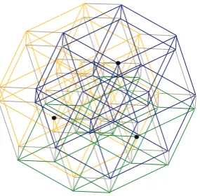
of{0,1}n. By merging the Hamming star-convex building blocks, we obtain the Hamming star-convexity packing as a consequence of the dynamics of neural networksseeFigure 2.
Theorem 4.1. LetX {x1, x2, . . . , xp}be a subset of{0,1}n. Then the phase space{0,1}ncan be
filled withp nonoverlapping Hamming star-convex sets withx1, x2, . . . , xp as star-centers,
respec-tively.
Proof. LetY {y1, y2, . . . , yq}be the kernel ofX. According toTheorem 3.1, we can construct
a neural network with a functionFencoding the dynamics such that the domains of attraction
DGSξ, whereξ ∈ 01-spanY, are the Hamming star-convex building blocks of {0,1}n. To
merge these Hamming star-convex building blocks, we establish first the following.
Assertion 4.2. For every x, y ∈ {0,1}n and for every v1, v2, . . . , vk ∈ Cx, y, there exist
u1, u2, . . . , uk∈Cx, ysuch that
Cx, yCu1, v1∪Cu2, v2∪ · · · ∪Cuk, vk,
Cui, vi∩Cuj, vj∅
4.1
for everyi, j ∈Æk withi /j.
It is clear that the assertion is valid for everyx, y∈ {0,1}nwithρHx, y 0. Assume that the assertion is valid for everyx, y∈ {0,1}nwithρHx, y p < n. Now letx, y∈ {0,1}n
withρHx, y p1. Chooseαso thatxα/yα, and use the complemented notation: 0 1, 10. Then, we have
Cx, yCxα, y∪Cx,yα, 4.2
Cxα, y∩Cx,yα∅, 4.3
Case 1. {v1, v2, . . . , vk} ∩Cxα, y ∅ or {v1, v2, . . . , vk} ∩Cx,yα ∅. We may assume thatv1, v2, . . . , vk ∈ Cxα, y. Then, by the induction hypothesis, there existu1, u2, . . . , uk ∈
Cxα, ysuch that
Cxα, yCu1, v1∪Cu2, v2∪ · · · ∪Cuk, vk, 4.4
Cui, vi∩Cuj, vj∅ 4.5
for everyi, j ∈Æk withi /j. For eachi∈Æk, let
uiαui
1, . . . , uiα−1, u i
α, uiα1, . . . , uin
,
viαvi
1, . . . , viα−1, v i
α, vαi1, . . . , vni
.
4.6
Sincexα/yα, it follows from4.4and4.5that
Cx,yαCu1α, v1α∪Cu2α,v2α∪ · · · ∪Cukα,vkα, 4.7
Cuiα,viα∩Cujα,vjα∅ 4.8
for everyi, j ∈Æk withi /j. Now combining4.2,4.4, and4.7with the property
Cui,viαCui, vi∪Cuiα,viα for eachi∈
Æk, 4.9
we obtain
Cx, yCu1,v1α∪Cu2,v2α∪ · · · ∪Cuk,vkα. 4.10
Moreover, it follows from4.3,4.5, and4.8that
Cui,viα∩Cuj,vjα∅ 4.11
for everyi, j ∈Æk withi /j.
Case 2. {v1, v2, . . . , vk} ∩Cxα, y/∅and{v1, v2, . . . , vk} ∩Cx,yα/∅. We may assume that
v1, v2, . . . , vs ∈Cxα, yandvs1, vs2, . . . , vk ∈Cx,yα, wheres∈
Æk. Then, by4.2,4.3,
and the induction hypothesis, there exist u1, u2, . . . , us ∈ Cxα, yand us1, us2, . . . , uk ∈
Cx,yαsuch that
Cx, yC
u1, v1
∪C
u2, v2
∪ · · · ∪C
uk, vk
,
Cui, vi∩Cuj, vj∅
for everyi, j ∈Æk withi /j, completing the inductive proof of the assertion.
Applying now the assertion toCx, y {0,1}nand the given pointsx1, x2, . . . , xp, we obtainu1, u2, . . . , ur such that
{0,1}nCu1, x1∪Cu2, x2∪ · · · ∪Cup, xp,
Cui, xi∩Cuj, xj∅
4.13
for everyi, j ∈Æp withi /j. For eachk∈Æp, define
Ωk01-spanY∩Cuk, xk. 4.14
Then,Ωk/∅for eachk∈Æp, since 01-spanY∈ΛX.
Claim 4.3. For eachk ∈ Æp, the set
ξ∈ΩkDGSξis Hamming star-convex withx
k as a star
center.
Fix k ∈ Æp and write x
k q
i1γiyi, where γi ∈ {0,1} for each i ∈ Æq. Let z ∈
ξ∈ΩkDGSξ. Then, there existsy∈Ωksuch thatz∈DGSy. Writey
q
i1αiyi, whereαi∈ {0,1}for eachi∈ Æq. Then, by3.14, there existz
0 ∈C0,
ÁYandz
i ∈C0, yifor each
i∈Æq such thatzz
0q
i1αizi. We have to show that
Cz, xk⊂
ξ∈Ωk∩Cy,xk
DGSξ. 4.15
Letv∈Cz, xk. Then, by2.18, there existv0 ∈C0,
ÁY,v
i ∈C0, yi, andβ
i ∈ {0,1}for eachi∈Æq such thatvv
0q
i1βivi. Sincev∈Cz, xk, we have
dv, xkv0
q
i1
dβivi, γiyi
≤z0
q
i1
dαizi, γiyi
dz, xk.
4.16
SinceY is orthogonal,4.16implies that
dβivi, γiyi
≤dαizi, γiyi
4.17
for eachi∈Æq. Moreover, we have the following inequalities:
Figure 2: The proof given in Theorem 4.1 reveals a merging process of the Hamming star-convexity packing. Here the 6-cube is filled with 3 nonoverlapping Hamming star-convex sets with star-centers spa-tially distributed in three vertices.
To show4.18, fixi∈Æqand consider only two cases.
Case 1αiγi1. Sincezi∈C0, yi,4.17implies that
d
βivi, yi
≤d
zi, yi
< yi. 4.19
Sincevi∈C0, yi,4.19implies thatβi 1, proving4.18.
Case 2αi γi 0. Then, by4.17, we havedβivi,0≤0. Sincevi ∈C0, yi, we getβi 0,
proving4.18.
Now combining4.18with the equality
dy, xk
q
i1
dαiyi, γiyi
q
i1
αi−γiyi 4.20
shows thatqi1βiyi∈Cy, xk, and hence that q
i1βiyi∈Ωk∩Cy, xk. On the other hand, by3.14, we havev∈DGSiq1βiyi, and that4.15holds.
Using the fact that
ξ∈Ωk∩Cy,xk
DGSξ⊂
ξ∈Ωk
DGSξ, 4.21
the claim follows. Combining the claim with4.13,4.14, and3.14proves the theorem.
5. Discussion
whose equilibrium states contain the prototypes. A common qualitative property, namely, the Hamming star-convexity, can be deduced from all those domains of attraction of equilibrium states and a merging process, which preserves the Hamming star-convexity, can also be determined. As a result, the phase space can be filled with nonoverlapping Hamming star-convex sets with all the star-centers exactly being the prototypes.
The design of the Hamming star-convexity packing can be used as a testbed for exploring the plasticity regimes that guides the evolution of the primitive Hopfield network. Indeed, we consider the evolutionary neural network whose dynamics is encoded by the nonlinear parametric equations31:
xt1 HAt,stxt, t0,1, . . . ,
At1 At Dxt→xt1A, t0,1, . . . ,
5.1
wheretis time,xt x1t, x2t, . . . , xntis the neuronal activity state at timet,At
aijtn×nis the evolutionary coupling state at timet,st∈ {1,2, . . . , n}denotes the neuron that adjusts its activity at timet,HAt,stxis the time-and-state varying function whoseith
component is defined byxiifi /st, otherwise n
j1aijtxj−bi, and eachDxt→xt1Ais
ann-by-nreal matrix whosei, j-entry is a plasticity parameter representing a choice of real
numbers based on algorithmic Hebbian synaptic plasticity. In31, we have shown that for
each domainΔ⊂ {0,1}n\ {0}and for each choice of initial neuronal activity statex0∈Δ,
there exists a plasticity regime that guides the dynamics of the evolutionary coupling states such thatxtconverges andxt∈Δfor everyt0,1, . . .. The plasticity regime, even when insoluble in the information storage scheme by assigningA0to be the matrix of synaptic strengths of the primitive Hopfield network given inTheorem 3.1andΔto be the Hamming star-convex set given inTheorem 4.1, is a guide to understand and explain the dynamism role of the Hamming star-convexity packing in storage and retrieval of associative memory.
Acknowledgment
This work was supported by the National Science Council of the Republic of China.
References
1 E. R. Kandel, “The molecular biology of memory storage: a dialog between genes and synapses,” in Nobel Lectures, Physiology or Medicine 1996–2000, H. Jornvall, Ed., pp. 392–439, World Scientific, Singapore, 2003.
2 B. Milner, L. R. Squire, and E. R. Kandel, “Cognitive neuroscience and the study of memory,”Neuron, vol. 20, no. 3, pp. 445–468, 1998.
3 D. O. Hebb,The Organization of Behavior, Wiley, New York, NY, USA, 1949.
4 J. A. Anderson, “A simple neural network generating an interactive memory,” Mathematical Biosciences, vol. 14, no. 3-4, pp. 197–220, 1972.
5 M. Cottrell, “Stability and attractivity in associative memory networks,”Biological Cybernetics, vol. 58, no. 2, pp. 129–139, 1988.
6 T. Kohonen, “Correlation matrix memories,”IEEE Transactions on Computers, vol. C-21, no. 4, pp. 353– 359, 1972.
7 G. Palm, “On associative memory,”Biological Cybernetics, vol. 36, no. 1, pp. 19–31, 1980.
9 D. J. Willshaw, O. P. Buneman, and H. C. Longuet-Higgins, “Non-holographic associative memory,” Nature, vol. 222, no. 5197, pp. 960–962, 1969.
10 S. Grossberg, “Nonlinear neural networks: principles, mechanisms, and architectures,” Neural Networks, vol. 1, no. 1, pp. 17–61, 1988.
11 S. Grossberg, “How does the cerebral cortex work? Learning, attention, and groupings by the laminar circuits of visual cortex,”Spatial Vision, vol. 12, no. 2, pp. 163–185, 1999.
12 J. Hertz, A. Krogh, and R. G. Palmer,Introduction to the Theory of Neural Computation, Santa Fe Institute Studies in the Sciences of Complexity. Lecture Notes, I, Addison-Wesley, Redwood City, Calif, USA, 1991.
13 J. J. Hopfield, “Neural networks and physical systems with emergent collective computational abilities,”Proceedings of the National Academy of Sciences of the United States of America, vol. 79, no. 8, pp. 2554–2558, 1982.
14 P. Peretto, “Collective properties of neural networks: a statistical physics approach,” Biological Cybernetics, vol. 50, no. 1, pp. 51–62, 1984.
15 G. Weisbuch, Complex Systems Dynamics: An Introduction to Automata Networks, Santa Fe Institute Studies in the Sciences of Complexity. Lecture Notes, II, Addison-Wesley, Redwood City, Calif, USA, 1991.
16 J. J. Hopfield and D. W. Tank, ““Neural” computation of decisons in optimization problems,” Biological Cybernetics, vol. 52, no. 3, pp. 141–152, 1985.
17 T.-D. Chiueh and R. M. Goodman, “Recurrent correlation associative memories,”IEEE Transactions on Neural Networks, vol. 2, no. 2, pp. 275–284, 1991.
18 C. Garc´ıa and J. A. Moreno, “The Hopfield associative memory network: improving performance with the kernel “trick”,” inProceedings of the 9th Ibero-American Conference on AI: Advances in Artificial Intelligence (IBERAMIA ’04), vol. 3315 ofLecture Notes in Artificial Intelligence, pp. 871–880, November 2004.
19 H. Gutfreund, “Neural networks with hierarchically correlated patterns,”Physical Review A, vol. 37, no. 2, pp. 570–577, 1988.
20 M. Hirahara, N. Oka, and T. Kindo, “Associative memory with a sparse encoding mechanism for storing correlated patterns,”Neural Networks, vol. 10, no. 9, pp. 1627–1636, 1997.
21 R. Perfetti and E. Ricci, “Recurrent correlation associative memories: a feature space perspective,” IEEE Transactions on Neural Networks, vol. 19, no. 2, pp. 333–345, 2008.
22 Y. Kamp and M. Hasler,Recursive Neural Networks for Associative Memory, Wiley-Interscience Series in Systems and Optimization, John Wiley & Sons, Chichester, UK, 1990.
23 T. Kohonen,Self-Organization and Associative Memory, vol. 8 ofSpringer Series in Information Sciences, Springer, Berlin, Germany, 2nd edition, 1988.
24 L. Personnaz, I. Guyon, and G. Dreyfus, “Collective computational properties of neural networks: new learning mechanisms,”Physical Review A, vol. 34, no. 5, pp. 4217–4228, 1986.
25 S. Diederich and M. Opper, “Learning of correlated patterns in spin-glass networks by local learning rules,”Physical Review Letters, vol. 58, no. 9, pp. 949–952, 1987.
26 M. Opper, “Learning times of neural networks: exact solution for a PERCEPTRON algorithm,” Physical Review A, vol. 38, no. 7, pp. 3824–3826, 1988.
27 Y. Shrivastava, S. Dasgupta, and S. M. Reddy, “Guaranteed convergence in a class of Hopfield networks,”IEEE Transactions on Neural Networks, vol. 3, no. 6, pp. 951–961, 1992.
28 M. K. M ¨uezzino ˘glu and C. G ¨uzelis¸, “A Boolean Hebb rule for binary associative memory design,” IEEE Transactions on Neural Networks, vol. 15, no. 1, pp. 195–202, 2004.
29 M.-H. Shih and J.-L. Ho, “Solution of the Boolean Markus-Yamabe problem,”Advances in Applied Mathematics, vol. 22, no. 1, pp. 60–102, 1999.
30 M.-H. Shih and J.-L. Dong, “A combinatorial analogue of the Jacobian problem in automata networks,”Advances in Applied Mathematics, vol. 34, no. 1, pp. 30–46, 2005.
31 M.-H. Shih and F.-S. Tsai, “Growth dynamics of cell assemblies,”SIAM Journal on Applied Mathematics, vol. 69, no. 4, pp. 1110–1161, 2009.
32 M. A. Cohen and S. Grossberg, “Absolute stability of global pattern formation and parallel memory storage by competitive neural networks,”IEEE Transactions on Systems, Man, and Cybernetics, vol. 13, no. 5, pp. 815–826, 1983.
34 T. Ando and M.-H. Shih, “Simultaneous contractibility,”SIAM Journal on Matrix Analysis and Applica-tions, vol. 19, no. 2, pp. 487–498, 1998.
35 A. Jadbabaie, J. Lin, and A. S. Morse, “Coordination of groups of mobile autonomous agents using nearest neighbor rules,”IEEE Transactions on Automatic Control, vol. 48, no. 6, pp. 988–1001, 2003.
36 M.-H. Shih and C.-T. Pang, “Simultaneous Schur stability of interval matrices,”Automatica, vol. 44, no. 10, pp. 2621–2627, 2008.
37 W. S. McCulloch and W. Pitts, “A logical calculus of the ideas immanent in nervous activity,”Bulletin of Mathematical Biophysics, vol. 5, pp. 115–133, 1943.
38 F. Robert,Discrete Iterations: A Metric Study, vol. 6 ofSpringer Series in Computational Mathematics, Springer, Berlin, Germany, 1986.
39 F. Robert, Les syst`emes dynamiques discrets, vol. 19 of Mathematics & Applications, Springer, Berlin, Germany, 1995.
40 R. W. Hamming, “Error detecting and error correcting codes,”The Bell System Technical Journal, vol. 29, pp. 147–160, 1950.