A hybrid iterative method for a combination of equilibria problem, a combination of variational inequality problems and a hierarchical fixed point problem

R E S E A R C H

Open Access

A hybrid iterative method for a combination

of equilibria problem, a combination of

variational inequality problems and a

hierarchical fixed point problem

Abdellah Bnouhachem

*_{Correspondence:}

[email protected] School of Management and Engineering, Nanjing University, Nanjing, 210093, P.R. China ENSA, Ibn Zohr University, BP 1136, Agadir, Morocco

Abstract

In this paper, we introduce and analyze a general iterative algorithm for finding a common solution of a combination of variational inequality problems, a combination of equilibria problem, and a hierarchical fixed point problem in the setting of real Hilbert space. Under appropriate conditions we derive the strong convergence results for this method. Several special cases are also discussed. Preliminary numerical experiments are included to verify the theoretical assertions of the proposed method. The results presented in this paper extend and improve some well-known results in the literature.

MSC: 49J30; 47H09; 47J20

Keywords: combination of equilibria problem; variational inequality; hierarchical fixed point problem; fixed point problem; projection method

1 Introduction

LetHbe a real Hilbert space, whose inner product and norm are denoted by·,·and · . LetCbe a nonempty closed convex subset ofH. LetF:C×C→Rbe a bifunction, the

equilibrium problem is to findx∈Csuch that

F(x,y)≥, ∀y∈C, (.)

which was considered and investigated by Blum and Oettli []. The solution set of (.) is denoted byEP(F). Equilibrium problems theory provides us with a unified, natural,

innovative, and general framework to study a wide class of problems arising in finance, economics, network analysis, transportation, elasticity, and optimization. This theory has witnessed an explosive growth in theoretical advances and applications across all disci-plines of pure and applied sciences; see [–].

IfF(u,v) =Au,v–u, whereA:C→His a nonlinear operator, then problem (.) is

equivalent to finding a vectoru∈Csuch that

v–u,Au ≥, ∀v∈C, (.)

which is known as the classical variational inequality. The solution of (.) is denoted by

VI(C,A). It is easy to observe that

u∗∈VI(C,A) ⇐⇒ u∗=PC

u∗–ρAu∗, whereρ> .

Variational inequalities are being used as a mathematical programming tool in modeling a large class of problems arising in various branches of pure and applied sciences. In recent years, variational inequalities have been generalized and extended novel and new tech-niques in several directions. We now have a variety of techtech-niques to suggest and analyze various iterative algorithms for solving variational inequalities and related optimization problems; see [–].

Fori= , , . . . ,N, letFi:C×C→Rbe bifunctions and ai∈(, ) with N

i=ai= .

Define the mappingN_i=aiFi:C×C→R. The combination of equilibria problem is to

findx∈Csuch that

N

i=

aiFi(x,y)≥, ∀y∈C, (.)

which was considered and investigated by Suwannaut and Kangtunyakarn []. The set of solutions (.) is denoted by

EP _N

i=

aiFi

=

N

i= EP(Fi).

IfFi=F,∀i= , , . . . ,N, then the combination of equilibria problem (.) reduces to the

equilibrium problem (.).

Fori= , , . . . ,N, letAibe a strongly positive linear bounded operator on a Hilbert space

H with coefficientρi>  andbi∈(, ) with N

i=bi= . The combination of variational

inequality problems is to findx∈Csuch that

N

i=

biAix,y–x

≥, ∀y∈C. (.)

If Ai=A, ∀i= , , . . . ,N, then the combination of variational inequality problems (.)

reduces to the variational inequality problem (.).

We introduce the following definitions, which are useful in the following analysis.

Definition . The mappingT:C→His said to be (a) monotone if

Tx–Ty,x–y ≥, ∀x,y∈C;

(b) strongly monotone if there existsα> such that

(c) strongly positive linear bounded if there existsα> such that

Tx,x ≥αx, ∀x∈C;

(d) nonexpansive if

Tx–Ty ≤ x–y, ∀x,y∈C;

(e) k-Lipschitz continuous if there exists a constantk> such that

Tx–Ty ≤kx–y, ∀x,y∈C;

(f ) a contraction onCif there exists a constant≤k< such that

Tx–Ty ≤kx–y, ∀x,y∈C.

It is easy to observe that everyα-inverse-strongly monotoneT is monotone and Lips-chitz continuous. It is well known that every nonexpansive operatorT:H→Hsatisfies, for all (x,y)∈H×H, the inequality

x–T(x)–y–T(y),T(y) –T(x)≤

T(x) –x

–T(y) –y (.)

and therefore, we get, for all (x,y)∈H×Fix(T),

x–T(x),y–T(x)≤

T(x) –x



. (.)

The fixed point problem for the mappingTis to findx∈Csuch that

Tx=x. (.)

We denote byF(T) the set of solutions of (.). It is well known thatF(T) is closed and convex, andPF(T) is well defined.

LetS:C→Hbe a nonexpansive mapping. The following problem is called a hierarchi-cal fixed point problem: Findx∈F(T) such that

x–Sx,y–x ≥, ∀y∈F(T). (.)

In , Yaoet al.[] introduced the following strong convergence iterative algorithm to solve problem (.):

yn=βnSxn+ ( –βn)xn,

xn+=PC

αnf(xn) + ( –αn)Tyn

, ∀n≥,

(.)

wheref :C→His a contraction mapping and{αn}and{βn}are two sequences in (, ).

Under some certain restrictions on the parameters, Yaoet al.proved that the sequence {xn}generated by (.) converges strongly toz∈F(T), which is the unique solution of the

following variational inequality:

(I–f)z,y–z≥, ∀y∈F(T). (.)

In , Cenget al.[] investigated the following iterative method:

xn+=PC

αnρU(xn) + (I–αnμF)

T(yn)

, ∀n≥, (.)

whereUis a Lipschitzian mapping, andFis a Lipschitzian and strongly monotone map-ping. They proved that under some approximate assumptions on the operators and pa-rameters, the sequence{xn}generated by (.) converges strongly to the unique solution

of the variational inequality

ρU(z) –μF(z),x–z≥, ∀x∈Fix(T). (.)

Very recently, in , Wang and Xu [] investigated an iterative method for a hierarchi-cal fixed point problem by

yn=βnSxn+ ( –βn)xn,

xn+=PC

αnρU(xn) + (I–αnμF)

T(yn)

, ∀n≥,

(.)

whereS:C→Cis a nonexpansive mapping. They proved that under some approximate assumptions on the operators and parameters, the sequence{xn}generated by (.)

con-verges strongly to the unique solution of the variational inequality (.).

In this paper, motivated by the work of Cenget al.[, ], Yaoet al.[], Wang and Xu [], Bnouhachem [, ] and by the recent work going in this direction, we give an iter-ative method for finding the approximate element of the common set of solutions of (.), (.), and (.) in a real Hilbert space. We establish a strong convergence theorem based on this method. We would like to mention that our proposed method is quite general and flexible and includes many known results for solving of variational inequality problems, equilibrium problems, and hierarchical fixed point problems; see,e.g., [, , , , , ] and relevant references cited therein.

2 Preliminaries

Lemma . Let PCdenote the projection of H onto C.Then we have the following

inequal-ities:

z–PC[z],PC[z] –v

≥, ∀z∈H,v∈C; (.)

u–v,PC[u] –PC[v]

≥PC[u] –PC[v] 

, ∀u,v∈H; (.)

PC[u] –PC[v]≤ u–v, ∀u,v∈H; (.)

u–PC[z]≤ z–u–z–PC[z], ∀z∈H,u∈C. (.)

Assumption .[] LetF:C×C→Rbe a bifunction satisfying the following

assump-tions:

(A) F(x,x) = ,∀x∈C;

(A) Fis monotone,i.e.,F(x,y) +F(y,x)≤,∀x,y∈C;

(A) for eachx,y,z∈C,limt→F(tz+ ( –t)x,y)≤F(x,y);

(A) for eachx∈C,y→F(x,y)is convex and lower semicontinuous.

Lemma .[] Let C be a nonempty closed convex subset of H.Let F:C×C→Rsatisfy

(A)-(A).Assume that for r> and∀x∈H,define a mapping Tr:H→C as follows:

Tr(x) =

z∈C:F(z,y) +



ry–z,z–x ≥,∀y∈C

.

Then the following hold:

(i) Tris nonempty and single-valued;

(ii) Tris firmly nonexpansive,i.e.;

Tr(x) –Tr(y) 

≤Tr(x) –Tr(y),x–y

, ∀x,y∈H;

(iii) F(Tr) =EP(F);

(iv) EP(F)is closed and convex.

Lemma .[] Let C be a nonempty closed convex subset of a real Hilbert space H.For i= , , . . . ,N,let Fi:C×C→Rbe bifunctions satisfying(A)-(A)withNi=EP(Fi)=∅.

ThenN_i=aiFisatisfies(A)-(A)and

Fix(Tr) =EP _N

i=

aiFi

=

N

i= EP(Fi),

where ai∈(, )for i= , , . . . ,N and N

i=ai= .

Lemma .[] Let C be a nonempty closed convex subset of a real Hilbert space H. If T :C→C is a nonexpansive mapping withFix(T)=∅, then the mapping I–T is demiclosed at,i.e.,if{xn}is a sequence in C weakly converging to x,and if{(I–T)xn}

Lemma .[] Let U:C→H be aτ-Lipschitzian mapping, and let F:C→H be a k-Lipschitzian andη-strongly monotone mapping,then for≤ρτ<μη,μF–ρU isμη–

ρτ-strongly monotone,i.e.,

(μF–ρU)x– (μF–ρU)y,x–y≥(μη–ρτ)x–y, ∀x,y∈C.

Lemma .[] Suppose thatλ∈(, )andμ> .Let F:C→H be a k-Lipschitzian and η-strongly monotone operator.In association with a nonexpansive mapping T :C→C, define the mapping Tλ_{:C→H by}

Tλ_{x=Tx–λμFT(x), ∀x∈C.}

Then Tλ_{is a contraction providedμ<}η

k,that is,

Tλ_x–Tλ_{y≤( –λν)x–y, ∀x,y∈C,}

whereν=  – –μ(η–μk_).

Lemma .[] Assume that{an}is a sequence of nonnegative real numbers such that

an+≤( –υn)an+δn,

where{υn}is a sequence in(, )andδnis a sequence such that

() ∞_n=υn=∞;

() lim sup_n→∞δn/υn≤or ∞

n=|δn|<∞.

Thenlim_n→∞an= .

Lemma .[] Let C be a closed convex subset of H.Let{xn}be a bounded sequence in H.

Assume that

(i) the weakw-limit setww(xn)⊂Cwhereww(xn) ={x:xnix};

(ii) for eachz∈C,limn→∞xn–zexists.

Then{xn}is weakly convergent to a point in C.

Lemma .[] Let C be a nonempty closed convex subset of a real Hilbert space H.For every i= , , . . . ,N,let Aibe a strongly positive linear bounded operator on a Hilbert space

H with coefficientρi> ,i.e.,Aix,x ≥ρix,∀x∈H,andρ¯=mini=,,...,Nρi.Let{bi}Ni=⊆

(, )withN_i=bi= .Then the following properties hold:

(i) I–λN_i=biAi ≤ –λρ¯andI–λ N

i=biAiis a nonexpansive mapping for every <λ<Ai–(i= , , . . . ,N).

(ii) VI(C,N_i=biAi) = N

i=VI(C,Ai).

3 The proposed method and some properties

In this section, we suggest and analyze our method for finding common solutions of the combination of equilibria problem (.), the combination of variational inequality prob-lems (.), and the hierarchical fixed point problem (.).

bounded operator on a Hilbert spaceHwith coefficientρi>  andρ¯=mini=,,...,Nρi, and

let S,T :C→Cbe nonexpansive mappings such that F(T)∩N_i=EP(Fi)∩Ni=VI(C,

Ai)=∅. LetF:C→Cbe ak-Lipschitzian mapping and beη-strongly monotone, and let

U:C→Cbe aτ-Lipschitzian mapping.

Algorithm . For an arbitrarily givenx∈C, let the iterative sequences{un},{xn},{yn},

and{zn}be generated by ⎧

⎪ ⎪ ⎪ ⎪ ⎨ ⎪ ⎪ ⎪ ⎪ ⎩

N

i=aiFi(un,y) +_r_ny–un,un–xn ≥, ∀y∈C;

zn=PC[un–λn N

i=biAiun];

yn=βnSxn+ ( –βn)un;

xn+=γnxn+ ( –γn)PC[αnρU(xn) + (I–αnμF)(T(yn))], ∀n≥.

(.)

Suppose that the parameters satisfy  <μ<_kη, ≤ρτ<ν, whereν= –

 –μ(η–μk_).

Also{γn},{αn},{βn}, and{rn}are sequences in (, ) satisfying the following conditions:

(a)  <a≤γn≤b< ,

(b) limn→∞αn= and ∞

n=αn=∞,

(c) limn→∞(βn/αn) = ,

(d) N_i=ai= N

i=bi= ,

(e) ∞_n=|αn––αn|<∞, ∞

n=|γn––γn|<∞, and ∞

n=|βn––βn|<∞,

(f ) lim infn→∞rn> and ∞

n=|rn––rn|<∞,

(g) lim_n→∞λn= and ∞

n=|λn––λn|<∞.

If fori= , , . . . ,N,Fi=FandAi=A, then Algorithm . reduces to Algorithm . for

finding the common solutions of equilibrium problem (.), variational inequality problem (.) and the hierarchical fixed point problem (.).

Algorithm . For an arbitrarily givenx∈Carbitrarily, let the iterative sequences{un},

{xn},{yn}, and{zn}be generated by ⎧

⎪ ⎪ ⎪ ⎪ ⎨ ⎪ ⎪ ⎪ ⎪ ⎩

F(un,y) +_r_ny–un,un–xn ≥, ∀y∈C;

zn=PC[un–λnAun];

yn=βnSxn+ ( –βn)zn;

xn+=γnxn+ ( –γn)PC[αnρU(xn) + (I–αnμF)(T(yn))], ∀n≥.

Suppose that the parameters satisfy  <μ<_kη, ≤ρτ<ν, whereν= –

 –μ(η–μk_).

Also{γn},{αn},{βn}, and{rn}are sequences in (, ) satisfying the following conditions:

(a)  <a≤γn≤b< ,

(b) limn→∞αn= and ∞

n=αn=∞,

(c) limn→∞(βn/αn) = ,

(d) ∞_n=|αn––αn|<∞,∞n=|γn––γn|<∞, and∞n=|βn––βn|<∞,

(e) lim infn→∞rn> and ∞

n=|rn––rn|<∞,

(f ) limn→∞λn= and ∞

n=|λn––λn|<∞.

• Ifγn= , the proposed method is an extension and improvement of the method of

Wang and Xu [] and Bnouhachem [] for finding the approximate element of the common set of solutions of a combination of variational inequality problems, a combination of equilibria problem and a hierarchical fixed point problem in a real Hilbert space.

• If we have the Lipschitzian mappingU=f,F=I,ρ=μ= , andγn= , we obtain an

extension and improvement of the method of Yaoet al.[] for finding the

approximate element of the common set of solutions of a combination of variational inequality problems, a combination of equilibria problem and a hierarchical fixed point problem in a real Hilbert space.

• The contractive mappingf with a coefficientα∈[, )in other papers [, , ] is extended to the cases of the Lipschitzian mappingUwith a coefficient constant γ ∈[,∞).

This shows that Algorithm . is quite general and unifying.

Lemma . Let x∗∈F(T)∩_i=N EP(Fi)∩Ni=VI(C,Ai).Then{xn},{un},{zn},and{yn}

are bounded.

Proof Letx∗∈F(T)∩N_i=EP(Fi)∩ N

i=VI(C,Ai); we havex∗=Trn(x∗). It follows from Lemmas . and . thatun=Trn(xn). SinceTrnis nonexpansive mapping, we have

un–x∗≤xn–x∗. (.)

Sincelimn→∞λn= , without loss of generality, we may assume that  <λn<Ai–,∀n≥

 andi= , , . . . ,N, by Lemma ., the mappingI–λnNi=biAiis nonexpansive mapping,

and we have

zn–x∗= PC

un–λn N

i=

biAiun

–PC

x∗–λn N

i=

biAix∗

≤

I–λn N

i=

biAi

un–

I–λn N

i=

biAi

x∗

≤un–x∗

≤xn–x∗. (.)

We defineVn=αnρU(xn) + (I–αnμF)(T(yn)). Next, we prove that the sequence{xn}is

bounded, and without loss of generality we can assume thatβn≤αnfor alln≥. From

(.), we have

xn+–x∗=γn

xn–x∗

+ ( –γn)

PC[Vn] –PC

x∗

≤γnxn–x∗+ ( –γn)αnρU(xn) + (I–αnμF)

T(yn)

–x∗

≤γnxn–x∗+ ( –γn)

αnρU(xn) –μF

x∗

+(I–αnμF)

T(yn)

– (I–αnμF)T

x∗

=γnxn–x∗+ ( –γn)

αnρU(xn) –ρU

+(I–αnμF)

T(yn)

– (I–αnμF)T

x∗

≤γnxn–x∗+ ( –γn)

αnρτxn–x∗

+αn(ρU–μF)x∗+ ( –αnν)yn–x∗

=γnxn–x∗+ ( –γn)

αnρτxn–x∗+αn(ρU–μF)x∗

+ ( –αnν)βnSxn+ ( –βn)zn–x∗

≤γnxn–x∗+αnρτ( –γn)xn–x∗+αn( –γn)(ρU–μF)x∗

+ ( –αnν)( –γn)

βnSxn–Sx∗+βnSx∗–x∗+ ( –βn)zn–x∗

≤γnxn–x∗+αnρτ( –γn)xn–x∗+αn( –γn)(ρU–μF)x∗

+ ( –αnν)( –γn)

βnSxn–Sx∗+βnSx∗–x∗+ ( –βn)xn–x∗

≤γnxn–x∗+αnρτ( –γn)xn–x∗+αn( –γn)(ρU–μF)x∗

+ ( –αnν)( –γn)

βnxn–x∗+βnSx∗–x∗+ ( –βn)xn–x∗

= –αn(ν–ρτ)( –γn)xn–x∗+αn( –γn)(ρU–μF)x∗

+ ( –αnν)( –γn)βnSx∗–x∗

≤ –αn(ν–ρτ)( –γn)xn–x∗

+αn( –γn)(ρU–μF)x∗+βn( –γn)Sx∗–x∗

≤ –αn(ν–ρτ)( –γn)xn–x∗

+αn( –γn)(ρU–μF)x∗+Sx∗–x∗

= –αn(ν–ρτ)( –γn)xn–x∗

+αn( –γn)(ν–ρτ)

ν–ρτ (ρU–μF)x

∗_+Sx∗_–x∗

≤maxxn–x∗,



ν–ρτ(ρU–μF)x

∗_+Sx∗_–x∗_,

where the third inequality follows from Lemma . and the fifth inequality follows from (.). By induction onn, we obtainxn–x∗ ≤max{x–x∗,_ν–_ρτ((ρU–μF)x∗+Sx∗–

x∗)}, forn≥ andx∈C. Hence,{xn}is bounded and consequently, we deduce that{un},

{zn},{vn},{yn},{S(xn)},{T(xn)},{F(T(yn))}, and{U(xn)}are bounded.

Lemma . Let x∗∈F(T)∩N_i=EP(Fi)∩ N

i=VI(C,Ai)and{xn}be the sequence

gener-ated by Algorithm..Then we have: (a) limn→∞xn+–xn= .

(b) The weakw-limit setww(xn)⊂F(T)(ww(xn) ={x:xnix}).

Proof From the nonexpansivity of the mappingI–λn N

i=biAiandPC, we have

zn–zn– ≤

un–λn N

i=

biAiun

–

un––λn– N

i=

biAiun–

=

un–λn N

i=

biAiun

–

un––λn N

i=

– (λn–λn–) N

i=

biAiun–

≤

un–λn N

i=

biAiun

–

un––λn N

i=

biAiun–

+|λn–λn–|

N

i=

biAiun–

≤ un–un–+|λn–λn–|

N

i=

biAiun–

. (.)

Next, we estimate that

yn–yn–=βnSxn+ ( –βn)zn–

βn–Sxn–+ ( –βn–)zn–

=βn(Sxn–Sxn–) + (βn–βn–)Sxn–

+ ( –βn)(zn–zn–) + (βn––βn)zn–

≤βnxn–xn–+ ( –βn)zn–zn–

+|βn–βn–|

Sxn–+zn–

. (.)

It follows from (.) and (.) that

yn–yn– ≤βnxn–xn–+ ( –βn)

un–un–+|λn–λn–|

N

i=

biAiun–

+|βn–βn–|

Sxn–+zn–

. (.)

On the other hand,un=Trn(xn) andun–=Trn–(xn–), we obtain

N

i=

aiFi(un,y) +

 rny

–un,un–xn ≥, ∀y∈C (.)

and

N

i=

aiFi(un–,y) +

 rn–y

–un–,un––xn– ≥, ∀y∈C. (.)

Takingy=un–in (.) andy=unin (.), we get

N

i=

aiFi(un,un–) +

 rn

un––un,un–xn ≥ (.)

and

N

i=

aiFi(un–,un) +

 rn–

Adding (.) and (.) and using the monotonicity ofN_i=aiFi, we have

un–un–,

un––xn–

rn–

–un–xn rn

≥,

which implies that

≤

un–un–,

rn

rn–

(un––xn–) – (un–xn)

=

un––un,un–un–+

 – rn rn–

un––xn+

rn

rn–

xn–

=

un––un,

 – rn rn–

un––xn+

rn

rn–

xn–

–un–un–

=

un––un,

 – rn rn–

(un––xn–) + (xn––xn)

–un–un–

≤ un––un

 – rn rn–

un––xn–+xn––xn

–un–un–

and then

un––un ≤  – rn

rn–

un––xn–+xn––xn.

Without loss of generality, let us assume that there exists a real numberχsuch thatrn>

χ>  for all positive integersn. Then we get

un––un ≤ xn––xn+



χ|rn––rn|un––xn–. (.)

It follows from (.) and (.) that

yn–yn– ≤βnxn–xn–+ ( –βn)

xn–xn–+



χ|rn–rn–|un––xn–

+|λn–λn–|

N

i=

biAiun–

+|βn–βn–|

Sxn–+zn–

=xn–xn–+ ( –βn)



χ|rn–rn–|un––xn–

+|λn–λn–|

N

i=

biAiun–

+|βn–βn–|

Sxn–+zn–

. (.)

Next, we estimate that

xn+–xn=γnxn+ ( –γn)PC[Vn]

–γn–xn–+ ( –γn–)PC[Vn–]

=γn(xn–xn–) + (γn–γn–)xn–+ ( –γn)

PC[Vn] –PC[Vn–]

≤γnxn–xn–+|γn–γn–|

xn–+PC[Vn–]

+ ( –γn)PC[Vn] –PC[Vn–]. (.)

Applying Lemma . to get

PC[Vn] –PC[Vn–]≤αnρ

U(xn) –U(xn–)

+ (αn–αn–)ρU(xn–)

+ (I–αnμF)

T(yn)

– (I–αnμF)T(yn–)

+ (I–αnμF)

T(yn–)

– (I–αn–μF)

T(yn–)

≤αnρτxn–xn–+ ( –αnν)yn–yn–

+|αn–αn–|ρU(xn–)+μF

T(yn–). (.)

From (.) and (.), we have

PC[Vn] –PC[Vn–]≤αnρτxn–xn–

+ ( –αnν)

xn–xn–+



μ|rn–rn–|un––xn–

+|λn–λn–|

N

i=

biAiun–

+|βn–βn–|

Sxn–+zn–

+|αn–αn–|ρU(xn–)+μF

T(yn–)

≤ – (ν–ρτ)αn

xn–xn–+



μ|rn–rn–|un––xn–

+|λn–λn–|

N

i=

biAiun–

+|βn–βn–|

Sxn–+zn–

+|αn–αn–|ρU(xn–)+μF

T(yn–). (.)

Substituting (.) into (.), we get

xn+–xn ≤

 – (ν–ρτ)( –γn)αn

xn–xn–+



μ|rn–rn–|un––xn–

+|λn–λn–|

N

i=

biAiun–

+|βn–βn–|

Sxn–+zn–

+|αn–αn–|ρU(xn–)+μF

T(yn–)

+|γn–γn–|

xn–+PC[Vn–]

≤ – (ν–ρτ)( –γn)αn

xn–xn–

+M



μ|rn–rn–|+|λn–λn–|+|βn–βn–|

+|αn–αn–|+|γn–γn–|

Here

M=max

sup n≥

un––xn–,sup n≥

N

i=

biAiun– ,supn≥

Sxn–+zn–

,

sup n≥

ρU(xn–)+μF

T(yn–),sup n≥

xn–+PC[Vn–]

.

It follows by conditions (a)-(b), (e)-(g) of Algorithm . and Lemma . that

lim

n→∞xn+–xn= .

Sincexn+–xn= ( –γn)(PC[Vn] –xn), we obtain

lim

n→∞PC[Vn] –xn= . (.)

Next, we show thatlimn→∞un–xn= . SinceTrnis firmly nonexpansive, we have un–x∗



=Trn(xn) –Trn

x∗

≤un–x∗,xn–x∗

= 

!un–x ∗

+xn–x∗ 

–un–x∗–

xn–x∗ "

.

Hence, we get

_un–x∗≤xn–x∗ 

–un–xn.

From (.) and the inequality above, we have

PC[Vn] –x∗ 

=PC[Vn] –x∗,PC[Vn] –x∗

=PC[Vn] –Vn,PC[Vn] –x∗

+Vn–x∗,PC[Vn] –x∗

≤αn

ρU(xn) –μF

x∗+ (I–αnμF)

T(yn)

– (I–αnμF)

Tx∗,PC[Vn] –x∗

=αnρ

U(xn) –U

x∗,PC[Vn] –x∗

+αn

ρUx∗–μFx∗,PC[Vn] –x∗

+(I–αnμF)

T(yn)

– (I–αnμF)

Tx∗,PC[Vn] –x∗

≤αnρτxn–x∗PC[Vn] –x∗+αn

ρUx∗–μFx∗,PC[Vn] –x∗

+ ( –αnν)yn–x∗PC[Vn] –x∗

≤ αnρτ

 xn–x ∗

+PC[Vn] –x∗

+αn

ρUx∗–μFx∗,PC[Vn] –x∗

+( –αnν)  yn–x

∗

≤ ( –αn(ν–ρτ))

 PC[Vn] –x ∗

+αnρτ  xn–x

∗

+αn

ρUx∗–μFx∗,PC[Vn] –x∗

+( –αnν) 

βnSxn–x∗ 

+ ( –βn)zn–x∗ 

≤ ( –αn(ν–ρτ))

 PC[Vn] –x ∗

+αnρτ  xn–x

∗

+αn

ρUx∗–μFx∗,PC[Vn] –x∗

+( –αnν)βn

 Sxn–x

∗

+( –αnν)( –βn)

 !xn–x

∗

–un–xn "

, (.)

which implies that

PC[Vn] –x∗≤

αnρτ

 +αn(ν–ρτ)

xn–x∗

+ αn

 +αn(ν–ρτ)

ρUx∗–μFx∗,PC[Vn] –x∗

+ ( –αnν)βn  +αn(ν–ρτ)

Sxn–x∗ 

+( –αnν)( –βn)  +αn(ν–ρτ)

!xn–x∗ 

–un–xn "

≤ αnρτ

 +αn(ν–ρτ)

xn–x∗ 

+ αn

 +αn(ν–ρτ)

ρUx∗–μFx∗,PC[Vn] –x∗

+ ( –αnν)βn  +αn(ν–ρτ)

Sxn–x∗ 

+xn–x∗–

( –αnν)( –βn)

 +αn(ν–ρτ)

un–xn.

Hence,

( –αnν)( –βn)

 +αn(ν–ρτ) un

–xn

≤ αnρτ

 +αn(ν–ρτ)

xn–x∗ 

+ αn

 +αn(ν–ρτ)

ρUx∗–μFx∗,PC[Vn] –x∗

+ ( –αnν)βn  +αn(ν–ρτ)

Sxn–x∗ 

+xn–x∗ 

–PC[Vn] –x∗ 

≤ αnρτ

 +αn(ν–ρτ)

xn–x∗ 

+ ( –αnν)βn  +αn(ν–ρτ)

Sxn–x∗ 

+ αn

 +αn(ν–ρτ)

ρUx∗–μFx∗,PC[Vn] –x∗

Sincelimn→∞PC[Vn] –xn= ,αn→,βn→, we obtain

lim

n→∞un–xn= . (.)

By (.) and the nonexpansivity of the mappingI–λn N

i=biAi, we get

zn–x∗ = PC

un–λn N

i=

biAiun

–PC

x∗–λn N

i=

biAix∗



≤ zn–x∗,

un–λn N

i=

biAiun

–

x∗–λn N

i=

biAix∗

=  

_zn–x∗+

I–λn N

i=

biAi

un–

I–λn N

i=

biAi x∗  –

un–x∗–λn _N

i=

biAiun– N

i=

biAix∗

–zn–x∗  ≤  

zn–x∗ 

+un–x∗ 

–

un–zn–λn _N

i=

biAiun– N

i=

biAix∗  ≤  

zn–x∗+un–x∗–un–zn

+ λn un–zn, N

i=

biAiun– N

i=

biAix∗

≤ 



zn–x∗+un–x∗–un–zn

+ λnun–zn N i=

biAiun– N

i=

biAix∗ . Hence

zn–x∗≤un–x∗–un–zn+ λnun–zn N i=

biAiun– N

i=

biAix∗

≤xn–x∗ 

–un–zn+ λnun–zn N i=

biAiun– N

i=

biAix∗ ,

where the second inequality follows from (.). From (.), and the inequality above, we have

PC[Vn] –x∗ 

≤ ( –αn(ν–ρτ))

 PC[Vn] –x ∗

+αnρτ  xn–x

∗

+αn

+( –αnν) 

βnSxn–x∗ 

+ ( –βn)zn–x∗ 

≤ ( –αn(ν–ρτ))

 PC[Vn] –x ∗

+αnρτ  xn–x

∗

+αn

ρUx∗–μFx∗,PC[Vn] –x∗

+( –αnν) 

βnSxn–x∗+ ( –βn)

xn–x∗

–un–zn+ λnun–zn N i=

biAiun– N

i=

biAix∗

,

which implies that

PC[Vn] –x∗ 

≤ αnρτ

 +αn(ν–ρτ)

xn–x∗ 

+ αn

 +αn(ν–ρτ)

ρUx∗–μFx∗,PC[Vn] –x∗

+ ( –αnν)βn  +αn(ν–ρτ)

Sxn–x∗ 

+( –αnν)( –βn)  +αn(ν–ρτ)

_xn–x∗–un–zn

+ λnun–zn N i=

biAiun– N

i=

biAix∗

≤ αnρτ

 +αn(ν–ρτ)

xn–x∗ 

+ ( –αnν)βn  +αn(ν–ρτ)

Sxn–x∗ 

+ αn

 +αn(ν–ρτ)

ρUx∗–μFx∗,PC[Vn] –x∗

+xn–x∗ 

+( –αnν)( –βn)  +αn(ν–ρτ)

–un–zn

+ λnun–zn N i=

biAiun– N

i=

biAix∗ . Hence,

( –αnν)( –βn)

 +αn(ν–ρτ)

un–zn

≤ αnρτ

 +αn(ν–ρτ)

xn–x∗ 

+ ( –αnν)βn  +αn(ν–ρτ)

Sxn–x∗ 

+ αn

 +αn(ν–ρτ)

ρUx∗–μFx∗,PC[Vn] –x∗

+xn–x∗ 

–PC[Vn] –x∗ 

+( –αnν)( –βn)  +αn(ν–ρτ)

λnun–zn N i=

biAiun– N

i=

≤ αnρτ

 +αn(ν–ρτ)

xn–x∗ 

+ ( –αnν)βn  +αn(ν–ρτ)

Sxn–x∗ 

+ αn

 +αn(ν–ρτ)

ρUx∗–μFx∗,PC[Vn] –x∗

+xn–x∗+PC[Vn] –x∗PC[Vn] –xn

+ λnun–zn

N

i=

biAiun– N

i=

biAix∗ .

Sincelimn→∞PC[Vn] –xn= ,αn→,βn→, andlimn→∞λn= , we obtain

lim

n→∞un–zn= . (.)

It follows from (.) and (.) that

lim

n→∞xn–zn= . (.)

SinceT(xn)∈C, we have

xn–T(xn)≤ xn–xn++xn+–T(xn)

=xn–xn++γn

xn–T(xn)

+ ( –γn)

PC[Vn] –T(xn)

≤ xn–xn++γnxn–T(xn)

+ ( –γn)αn

ρU(xn) –μF

T(yn)

+T(yn) –T(xn)

≤ xn–xn++γnxn–T(xn)

+αn( –γn)ρU(xn) –μF

T(yn)+ ( –γn)yn–xn

=xn–xn++γnxn–T(xn)+αn( –γn)ρU(xn) –μF

T(yn)

+ ( –γn)βnSxn+ ( –βn)zn–xn

≤ xn–xn++γnxn–T(xn)+αn( –γn)ρU(xn) –μF

T(yn)

+βn( –γn)Sxn–xn+ ( –βn)( –γn)zn–xn,

which implies that

_xn–T(xn)≤

  –γnxn

–xn++αnρU(xn) –μF

T(yn)

+βnSxn–xn+ ( –βn)zn–xn.

Sincelimn→∞xn+–xn= ,αn→,βn→, andρU(xn) –μF(T(yn))andSxn–xn

are bounded, andlim_n→∞zn–xn= , we obtain

lim

n→∞xn–T(xn)= .

Since{xn}is bounded, without loss of generality we can assume thatxnx∗∈C. It follows

Theorem . The sequence{xn}generated by Algorithm.converges strongly to z,which

is the unique solution of the variational inequality

ρU(z) –μF(z),x–z≤, ∀x∈F(T)∩

N

i= EP(Fi)

N

i=

VI(C,Ai). (.)

Proof Since{xn}is boundedxnwand from Lemma ., we havew∈F(T). Next, we

show thatw∈N_i=EP(Fi). Sinceun=Trn(xn), we have

N

i=

aiFi(un,y) +

 rn

y–un,un–xn ≥, ∀y∈C.

It follows from the monotonicity ofN_i=aiFithat

 rny

–un,un–xn ≥ N

i=

aiFi(y,un), ∀y∈C

and

y–unk,

unk–xnk

rnk

≥

N

i=

aiFi(y,unk), ∀y∈C. (.)

Sincelimn→∞un–xn= , andxnw, it is easy to observe thatunk →w. For any  <

t≤ andy∈C, letyt=ty+ ( –t)w, and let us haveyt∈C. Then from (.), we obtain

≥–

yt–unk,

unk–xnk

rnk

+

N

i=

aiFi(yt,unk). (.)

Sinceunk →w, it follows from (.) that

≥

N

i=

aiFi(yt,w). (.)

SinceN_i=aiFisatisfies (A)-(A), it follows from (.) that

 =

N

i=

aiFi(yt,yt)≤t N

i=

aiFi(yt,y) + ( –t) N

i=

aiFi(yt,w)

≤t

N

i=

aiFi(yt,y), (.)

which implies thatN_i=aiFi(yt,y)≥. Lettingt→+, we have

N

i=

aiFi(w,y)≥, ∀y∈C,

therefore,w∈EP(N_i=aiFi) = N

Furthermore, we show thatw∈N_i=VI(C,Ai). Let

Tv=

N

i=biAiv+NCv, ∀v∈C,

∅, otherwise,

whereNCv:={w∈H:w,v–u ≥,∀u∈C}is the normal cone toCatv∈C. ThenT

is maximal monotone and ∈Tvif and only ifv∈VI(C,N_i=biAi) (see []). LetG(T)

denote the graph ofT, and let (v,u)∈G(T); sinceu–_i=N biAiv∈NCvandzn∈C, we

have

v–zn,u– N

i=

biAiv

≥. (.)

It follows fromzn=PC[un–λn N

i=biAiun] andv∈Cthat

v–zn,zn–

un–λn N

i=

biAiun

≥

and

v–zn,

zn–un

λn

+

N

i=

biAiun

≥.

Therefore, from (.) and strongly positivity ofN_i=biAi, we have

v–znk,u ≥ v–znk, N

i=

biAiv

≥ v–znk, N

i=

biAiv

– v–znk,

znk–unk

λnk +

N

i=

biAiunk

= v–znk, N

i=

biAiv– N

i=

biAiznk

+ v–znk, N

i=

biAiznk– N

i=

biAiunk

–

v–znk,

znk–unk

λnk

= v–znk, N

i=

biAi(v–znk)

+ v–znk, N

i=

biAiznk– N

i=

biAiunk

–

v–znk,

znk–unk

λnk

≥ v–znk, N

i=

biAiznk– N

i=

biAiunk

–

v–znk,

znk–unk

λnk

.

VI(C,N_i=biAi) = N

i=VI(C,Ai). Thus we have

w∈F(T)∩

N

i=

EP(Fi)∩ N

i=

VI(C,Ai).

Observe that the constants satisfy ≤ρτ<νand

k≥η ⇐⇒ k≥η

⇐⇒  – μη+μk≥ – μη+μη

⇐⇒ # –μη–μk_{≥ –μη}

⇐⇒ μη≥ –

#

 –μη–μk

⇐⇒ μη≥ν,

therefore, from Lemma ., the operator μF–ρU isμη–ρτ strongly monotone, and we get the uniqueness of the solution of the variational inequality (.) and denote it by z∈F(T)∩N_i=EP(Fi)

N

i=VI(C,Ai).

Next, we claim thatlim sup_n→∞ρU(z) –μF(z),xn–z ≤. Since{xn}is bounded, there

exists a subsequence{xnk}of{xn}such that

lim sup n→∞

ρU(z) –μF(z),xn–z

=lim sup k→∞

ρU(z) –μF(z),xnk–z

=ρU(z) –μF(z),w–z≤.

By (.), we deduce

lim sup n→∞

ρU(z) –μF(z),PC[Vn] –z

≤lim sup n→∞

ρU(z) –μF(z),PC[Vn] –xn

+lim sup n→∞

ρU(z) –μF(z),xn–z

≤lim sup n→∞

ρU(z) –μF(z),xn–z

≤.

Next, we show thatxn→z. Note that PC[Vn] –z =

PC[Vn] –z,PC[Vn] –z

=PC[Vn] –Vn,PC[Vn] –z

+Vn–z,PC[Vn] –z

≤αn

ρU(xn) –μF(z)

+ (I–αnμF)

T(yn)

– (I–αnμF)

T(z),PC[Vn] –z

=αnρ

U(xn) –U(z)

,PC[Vn] –z

+αn

ρU(z) –μF(z),PC[Vn] –z

+(I–αnμF)

T(yn)

– (I–αnμF)

T(z),PC[Vn] –z

≤αnρτxn–zPC[Vn] –z+αn

ρU(z) –μF(z),PC[Vn] –z

≤αnρτxn–zPC[Vn] –z+αn

ρU(z) –μF(z),PC[Vn] –z

+ ( –αnν) !

βnSxn–Sz+βnSz–z

+ ( –βn)zn–z"PC[Vn] –z

≤αnρτxn–zPC[Vn] –z+αn

ρU(z) –μF(z),PC[Vn] –z

+ ( –αnν) !

βnxn–z+βnSz–z

+ ( –βn)xn–z"PC[Vn] –z

= –αn(ν–ρτ)

xn–zPC[Vn] –z

+αn

ρU(z) –μF(z),PC[Vn] –z

+ ( –αnν)βnSz–zPC[Vn] –z

≤  –αn(ν–ρτ)



xn–z+PC[Vn] –z 

+αn

ρU(z) –μF(z),PC[Vn] –z

+ ( –αnν)βnSz–zPC[Vn] –z,

which implies that

PC[Vn] –z 

≤  –αn(ν–ρτ)

 +αn(ν–ρτ)

xn–z

+ αn

 +αn(ν–ρτ)

ρU(z) –μF(z),PC[Vn] –z

+ ( –αnν)βn  +αn(ν–ρτ)

Sz–zPC[Vn] –z

≤ –αn(ν–ρτ)

xn–z

+ αn(ν–ρτ)  +αn(ν–ρτ)



ν–ρτ

ρU(z) –μF(z),PC[Vn] –z

+( –αnν)βn

αn(ν–ρτ)Sz

–zPC[Vn] –z

.

From (.) and the inequality above, we get

xn+–z≤γnxn–z+ ( –γn)PC(Vn) –z 

≤γnxn–z+

 –αn(ν–ρτ)

( –γn)xn–z

+αn( –γn)(ν–ρτ)  +αn(ν–ρτ)



ν–ρτ

ρU(z) –μF(z),PC[Vn] –z

+( –αnν)βn

αn(ν–ρτ)

Sz–zPC[Vn] –z

= –αn(ν–ρτ)( –γn)

xn–z

+αn( –γn)(ν–ρτ)  +αn(ν–ρτ)



ν–ρτ

ρU(z) –μF(z),PC[Vn] –z

+( –αnν)βn

αn(ν–ρτ)

Sz–zPC[Vn] –z

Let

υn=αn( –γn)(ν–ρτ)

and

δn=

αn( –γn)(ν–ρτ)

 +αn(ν–ρτ)



ν–ρτ

ρU(z) –μF(z),PC[Vn] –z

+( –αnν)βn

αn(ν–ρτ)Sz

–zPC[Vn] –z

.

We have

∞

n=

αn=∞

and

lim sup n→∞



ν–ρτ

ρU(z) –μF(z),PC[Vn] –z

+( –αnν)βn

αn(ν–ρτ)Sz

–zPC[Vn] –z

≤.

It follows that

∞

n=

υn=∞ and lim sup n→∞

δn

υn≤

.

Thus all the conditions of Lemma . are satisfied. Hence we deduce thatxn→z. This

completes the proof.

4 Applications

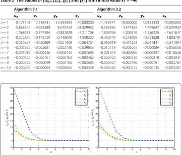
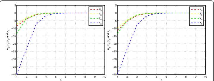
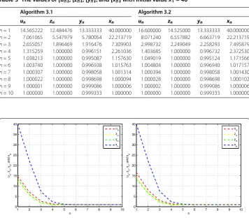
To verify the theoretical assertions, we consider the following examples.

Example . Letαn=_n ,γn=_n ,βn=_n,λn=_(n+) , andrn=_n+n .

We have

lim n→∞αn=

 nlim→∞

 n= 

and

∞

n=

αn=

 

∞

n=

 n=∞.

The sequence{αn}satisfies condition (b),

lim n→∞

βn

αn

= lim n→∞

 n = .

Condition (c) is satisfied. We compute

αn––αn=

 

 n– –

 n

= 

It is easy to show∞_n=|αn––αn|<∞. Similarly, we can show ∞

n=|γn––γn|<∞and ∞

n=|βn––βn|<∞. The sequences{αn},{γn}and{βn}satisfy condition (e). We have

lim inf

n→∞ rn=lim infn→∞

n n+ = 

and

∞

n=

|rn––rn|= ∞

n=

n_n– – n n+ 

= ∞

n=

 n(n+ )

≤

∞

n=

 n

< ∞.

Then the sequence{rn}satisfies condition (f ),

∞

n=

|λn––λn|= ∞

n=

__n–  (n+ )

=  

∞

n= _n– 

n+ 

≤ 

.

Then the sequence{λn}satisfies condition (g).

LetRbe the set of real numbers, and let the mappingT:R→Rbe defined by

T(x) =x

, ∀x∈R,

let the mappingF:R→Rbe defined by

F(x) =x+ 

 , ∀x∈R,

let the mappingS:R→Rbe defined by

S(x) =x

, ∀x∈R,

let the mappingU:R→Rbe defined by

U(x) = x

, ∀x∈R,

and, fori= , , . . . ,N, let the mappingAi:R→Rbe defined by

Aix=

ix

andbi=_i+_NN, and let the mappingFi:R×R→Rbe defined by

Fi(x,y) =i

–x+xy+ y, ∀(x,y)∈R×R

andai=_i+_N_N.

It is easy to show thatTandSare nonexpansive mappings,Fis a -Lipschitzian mapping and _-strongly monotone,Uis a_-Lipschitzian,Aiis a strongly positive linear bounded

operator, and theFisatisfy (A)-(A). It is clear that

F(T)∩

N

i=

EP(Fi)∩ N

i=

VI(C,Ai) ={}.

By the definition ofFi, we have

≤

N

i=

aiFi(un,y) +

 rny

–un,un–xn

=σ–u_n+uny+ y

+  rn

(y–un)(un–xn),

whereσ=N_i=(_i+ 

NN)i. Then

≤σrn

–u_n+uny+ y

+yun–yxn–un+unxn

= σrny+ (σrnun+un–xn)y– σrnun–un+unxn.

LetB(y) = σrny+ (σrnun+un–xn)y– σrnun–un+unxn.B(y) is a quadratic function

ofywith coefficienta= σrn,b=σrnun+un–xn,c= –σrnun–un+unxn. We determine

the discriminantofBas follows:

=b– ac

= (σrnun+un–xn)– σrn

–σrnun–un+unxn

=u_n+ σrnun+ σunrn– xnun– σxnunrn+xn

= (un+ σunrn)– xn(un+ σunrn) +xn

= (un+ σunrn–xn).

We haveB(y)≥,∀y∈R. If it has at most one solution inR, then= , we obtain

un=

xn

 + σrn

. (.)

For everyn≥, from (.), we rewrite (.) as follows:

⎧ ⎪ ⎨ ⎪ ⎩

zn=_+xnσrn– N

i=bi_{(n+)(+}ixn σrn);

yn=_nxn + ( –_n)zn;