Application of Mean-Square Approximation for Piecewise Linear Optimal Compander Design for Gaussian Source and Gaussian Mixture Model

Application of Mean-Square Approximation for Piecewise Linear Optimal

Compander Design for Gaussian Source and Gaussian Mixture Model

Zoran Perić

1

_{, Jelena Lukić}

2

_{, Jelena Nikolić}

3

_{, Dragan Denić}

4

University of Niš, Faculty of Electronic Engineering, Aleksandra Medvedeva 14, 18000 Niš, Serbia

e-mail: [email protected], [email protected],

3_{[email protected],} 4_{[email protected]}

http://dx.doi.org/10.5755/j01.itc.42.3.4349

Abstract. This paper proposes a novel piecewise linear optimal compander design method based on the mean-square approximation of the first derivative of the optimal compressor function. Designing of the piecewise linear optimal compander is conducted for signals modeled with the Gaussian probability density function (PDF) and signals modeled with the Gaussian mixture model (GMM). The slopes of the piecewise linear optimal compressor function are optimized for each quantization segment from the support region. The optimization is performed with a goal of obtaining minimal mean-squared error introduced with the proposed approximation, in this manner affecting the number of the uniform cells within each segment. The obtained numerical results show that signal-to-quantization-noise ratio (SQNR) of so obtained piecewise linear optimal compander overreaches SQNR of the uniform quantizer, whereas approaches to the SQNR of the nonlinear optimal compander for higher number of quantization segments. Features of the proposed quantizer indicate great possibilities for its widespread application in quantization of signals modeled by Gaussian PDF and GMM.

Keywords: linearization; mean-square approximation; spline approximation; Gaussian PDF; Gaussian mixture model; SQNR.

1. Introduction

The quantization process represents mapping of an infinite set of signal samples into a finite one, which yields to information loss [11]. A great challenge in developing a novel quantizer model can be the minimization of this loss, i.e., the minimization of distortion as its measure. The knowledge and understanding of the properties of the existing quantizer models can provide improvement of novel quantizer solutions and can facilitate their application in signal processing. The analysis of different quantizer model properties usually begins with the consideration of the properties of the most common types of scalar quantizers, uniform and non-uniform ones. A uniform quantizer is known by its design simplicity [11]. For a given number of quantization levels and given non-uniform PDF of the input signal, a non-uniform quantizer less distorts the signal in comparison to a uniform quantizer [11]. Most of real signals have a uniform PDF, which is why non-uniform quantizers are frequently used. Generally, for the given PDF, quantizers can be optimized to yield the minimal distortion and there are two approaches proposed in the literature that are mostly used. One

uses computationally demanding Lloyd-Max’s algorithm that designs iteratively an optimal quantizer for a given PDF [5], [11]. The second approach yields an asymptotically optimal quantizer and is based on compression, uniform quantization and expansion of the input signal, where compression and expansion

functions are mutually inverse[11]. These three steps

piecewise linear optimal compander (PLOC) on the changing variance of the input signal was analyzed in [3] and [6]. Unlike the quantizer proposed in [6], where the number of cells were assumed to be constant per segment and where the segments were determined by the equidistant partition of the optimal compressor function, in [7] and [10] the number of cells per segment were optimized contributing to the distortion decrease. The fact that above-mentioned quantizers are piecewise linear, that is, simpler for designing and implementation compared to nonlinear quantizers, justifies their widespread application. For example, in widely used digital PCM (Pulse Code Modulation) system the compression and expansion characteristics are piecewise linear approximations to µ-law and A-law characteristics [11].

In this paper, the mean-square approximation of the first derivative of the optimal compressor function is applied in designing the quantizer and the performances of the developed quantizer are analyzed. This choice is made due to analytical simplicity and tractability of the applied approximation of the function’s first derivative instead of approximating the function itself. In this way, the design complexity of the quantizer model becomes lower compared to the complexity of the previously reported piecewise linear quantizer models. The above-mentioned advantages of the piecewise linear quantizers led to their more common application in smart sensors [4]. In order to achieve linear dependence between the measured values on the input of the transducer and A/D converter’s output, the nonlinear transfer characteristic of the quantizer in A/D converter is programmed to be the inverse characteristic to the one of the transducer [4]. With the suitable piecewise linearization of the quantizer’s transfer characteristic one can simplify the design of A/D converter implemented in smart sensors. To retain the linearity between the input of the transducer and A/D converter’s output, the nonlinear and the obtained piecewise linear characteristic should be fitted as close as possible [4]. In this paper, we propose a method which achieves this goal.

The majority of real signals from our environment, and among them speech signals, can be modeled with a Gaussian PDF or GMM [9]. In this paper we are mainly focused on PLOC designing for the Gaussian source. We also describe the PLOC designing procedure for the GMM. In particular, Section 2 contains detailed analytical derivations, given in the form of lemmas, describing the designing procedure of the PLOC for the Gaussian source. In Section 3 the designing procedure is conducted for the signals modeled with GMM. Section 4 reports the numerical results validating the conclusions derived in Section 5.

2. Design of the novel piecewise linear optimal

compander

This section describes the design of the novel PLOC for the Gaussian PDF of unit variance and zero mean value:

(

/2

)

exp 2 1 )

(x x2

p = −

p . (1)

For the given number of quantization levels N and the assumed Gaussian PDF, the optimal compander support region threshold xL is given by [12], [13]:

( )

(

_{( )}

( )

)

( )

_{( )}

    

  

− −

=

N N

N N

x_L

ln 2

3 ln ln

4 ln ln 1 ln

6

p

. (2)

The optimal compressor function c(x): [-xL, xL]→

[-xL, xL], derived for the assumed Gaussian PDF, has

the following form [11]:

(

)

(

)

(

)

(

)

     

      

 

≤ ≤ − −

− −

≤ ≤ −

−

=

∫

∫

∫

∫

−

0 ,

6 / exp

6 / exp

0 , 6 / exp

6 / exp

) (

0 2 0

2 0

2 0

2

x x

dt t

dt t

x

x x

dt t

dt t

x

x c

L

x x L

L x

x

L

L L

. (3)

In general, a compander is consisted of three

building blocks, a compressor c(·), a uniform

quantizer Q(c(·)) and an expander c-1(·) (see Fig. 1). For the assumed Gaussian source the optimal compressor performs numerical integration and the optimal expander solves integral equations, which make difficult the application of the optimal compander for the observed source. For that reason, a method for the optimal compander linearization can be of great importance. This is due to the ability of decreasing the complexity of compander design and providing a simpler application of the PLOC for the cases where the Gaussian PDF is assumed. From hardware point of view, it is important to obtain linear transfer characteristics, herein compressor and expander characteristics, which overcome the problem observed with accurately implementing analog nonlinearities [1].

Let us assume, as in [7] and [10], that the number of segments of the same width, constituting our piecewise linear optimal compander support region, is 2 L. Due to the quantizer symmetry, hereafter, only the positive part of the support region will be considered. The segment width of the quantizer we propose is determined by:

L x_L

i=

∆ =

The mean-square approximation of the optimal compressor function first derivative:

( )

exp

(

/6

)

' 2 0 x C x x

c = L − , 0≤x≤x_L, (5) we propose in this paper is of the form:

( )

(

)

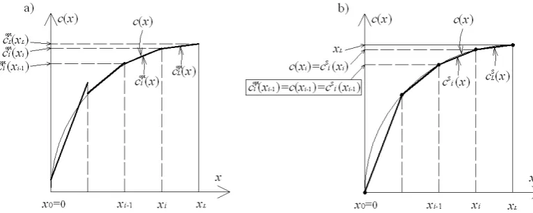
        ≤ ≤ < ≤ < ≤ ≅ − = − − L L L i i i L x x x a x x x a x x a x C x x c 1 1 1 1 2 0 , , 0 , 6 / exp '   ,(6)

Figure 1. The block diagram of a compander

where C0 is the constant given with:

(

t

)

dt

C L x

∫

− = 0 2

0 exp /6 . (7)

The parameter ai, for i = 1, …, L, represents the

slope of the piecewise linear optimal compressor function for the i-th linear segment [xi-1, xi). Towards

better understanding of the proposed approximation method and with the goal to provide better insight in details of the obtained linearized compander model, three basic features of the proposed approximation method are given and analyzed through the following lemmas.

Lemma 1: The optimal slopes aiopt of the piecewise

linear optimal compressor function obtained by the mean-square approximation of the first derivative of the optimal compressor function c'(x), are given with:

(

t

)

dt x x C x a i i x x i i L i

∫

− − − = − 1 6 / exp 1 2 1 0 opt _, . ,..., 1 L i= (8)

▼Proof: The first derivative of the optimal compressor function (3) is given by (5), for 0≤ x ≤ xL.

The mean-squared error, MSE, introduced with the

observed approximation of the first derivative of the optimal compressor function with corresponding constants ai, i = 1, …, L, is:

(

t

)

dt C x a x x F i i x x L i L

i i i

∫

∑

−       − − − =

= − ₁

2 2 0 1 1 6 / exp 1 . (9)

By minimizing F with respect to ai, i = 1, …, L,

the optimal slopes of the piecewise linear optimal compressor function are obtained. xi-1 and xi denotes

the thresholds of the i-th segment and ai is the slope of

the piecewise linear optimal compressor function for the i-th segment. Setting the first derivative of F with respect to ai equal to zero:

0 = ∂ ∂ i a F

, i=1,...,L, (10) leads to (8) and concludes Lemma1. ▲

Lemma 2: The slope asi of the first degree spline

approximation of the optimal compressor function for the i-th segment is equal to aiopt (8):

,

opt s

i i a

a = i=1,...,L. (11) ▼Proof: The slope of the first degree spline approximation for the i-th segment [xi-1, xi) can be

expresed by using the equation of a line passing through the points (xi-1, c

s

i(xi-1)) and (xi, c s

i(xi)):

( )

( )

1 1 s s s − − − − = i i i i i i i x x x c x c

a . (12)

Since the first degree spline approximation

function csi(x) matches the optimal compressor

function c(x) in xi-1 and xi [14] (see Fig. 2), the

previous exspression can be rewritten as follows:

( ) ( )

₍

₎

dt t x x C x x x x c x c a i i x x i i L i i i i i

∫

− − − = − − = − − − 1 6 / exp 1 2 1 0 1 1 s .(13)

By comparing (8) and (13) one can see that the statement of Lemma2 is correct.▲

Lemma 3: The proposed piecewise optimal

compressor function in general need not to be a continuous function. If the proposed function matches the first degree spline approximation of the optimal compressor function:

( )

x c

( )

x

ciopt = si , 0≤x≤xL, (14)

it is a continuous function.

▼Proof: Our piecewise linear optimal compressor function can be expressed with:

( )

opt ,

opt

i i i x a x d

c = + i=1,...,L, (15)

where coefficient di represents the ordinate axis

intercept for the i-th segment. From (15) it follows:

( )

opt ,

opt _{x a x}

c

d_i= _i − _i i=1,...,L. (16) By assuming that our piecewise linear optimal compressor function matches the optimal compressor function and spline function in points xi-1:

( ) ( )

_{1 1} ,

opt

−

− = i

i i x c x

c i=1,...,L, (17)

the coefficient di can be further expressed with:

( )

₋₁ − opt ₋₁,

= _{i i i}

i cx a x

Figure 2. (a) Piecewise linear optimal compressor function after application of the proposed approximation, (b) First degree spline approximation of the optimal compressor function

The first degree spline approximation of the optimal compressor function can be written as:

( )

s s,

s

i i i x a x d

c = + i=1,...,L, (19) where asi is defined by (13). To prove Lemma 3, we

have to show that the expressions (15) and (19) are identical at points xi-1, i = 1,..., L. Recall that it holds

asi = aiopt (11). This means that the proof of Lemma 3

ends with proving the equality of the coefficients dsi

and di, for x = xi-1. Going toward this goal, we give the

equation of a straight line passing through points (xi-1, c(xi-1)) and (xi, c(xi)):

( ) ( )

( ) ( )

1 1 s

1 1

− −

− −

− − = −

−

i i i

i i

i i

x x

x c x c x

x x c x c

. (20)

After subjecting the expression (20) to some simple modifications, the following is obtained:

( ) ( ) ( )(

−

) ( )

+ = −

−

= _{− −}

− −

1 1

1 1 s

i i

i i

i i

i x x c x

x x

x c x c x c

(

) ( )

(

( )

1

)

s 1 s

1 1

s

− −

−

− + = + −

−

=ai x xi cxi a ix cxi aixi . (21)

Finally, the first degree spline approximation of the optimal compressor function in xi-1 point has the form:

( )

_i i _i i

i x a x d

cs −₁ = s −₁+ s . (22)

Obviously, from (21) and (22) it follows:

( )

s ₁

1 s

−

− −

= _i i _i

i c x a x

d . (23)

Comparison of the expressions (18) and (23) reveals that coefficients di and dsi are equal, because of

equality of aiopt and asi. In the observed case the

proposed piecewise linear optimal compressor function and the first degree spline approximation matches and, accordingly, the proposed function is a continuous function. Conducting the previous conclusions proves Lemma 3. ▲

The optimal slope of the proposed piecewise linear optimal compressor function for the i-th (i = 1,..., L) segment, aiopt, defines the number of cells within the

i-th segment Ni/2 and the width of uniform cells δi:

( )

( )

( )

=

− −

= −

L L

i i i i i

x c

x c x c N N

opt

1 opt opt

2 2 2

(

)

L L L

i i i

d x a

x x a N

+ − −

= −

opt 1 opt

2 2

, i=1,...,L, (24)

i L

i i i

LN x N

2 2 / Δ ₌

=

δ , i=1,...,L. (25) As already mentioned, the segment thresholds are equidistant and can be expressed as:

L x i

x L

i = , i=0,...,L. (26)

The decision thresholds, i.e., the cell thresholds can be expressed in the following manner:

i i ij x j

x = ₋₁+

δ

, i=1,...,L, j=0,...,N_i/2. (27) The reproduction levels are similarly defined with:

i i

ij

j x

y δ

2 1 2

1

− +

= ₋ , i=1,...,L, j=1,...,Ni/2. (28)

The performance of a quantizer can be evaluated by determining the distortion as an inevitable error introduced in the signal during quantization. The overall distortion is a sum of a granular Dg and an

overload Dol distortion [11]. By definition of the

mean-squared error, Dg and Dol have the following

form [11]:

(

)

( )

∑ ∑ ∫

_{= =}

−

− =

L

i N

j x

x ij g

i ij

ij

dt t p y t D

1 2 /

1

2

1

2 , (29)

(

) ( )

∫

∞

− =

L x

ol

ol t y pt dt

D 2 2 , (30)

and the overall distortion D is:

ol g D

D

In the expression (29), xij-1 and xij are the

thresholds of the j-th cell, and yij is the reproduction

level from the j-th cell of the i-th segment. The

reproduction level yol from the overload region, which

is complementary to the support region, can be calculated as the centroid of the assumed PDF on [xL,

∞) [12], [13]:

( )

( )

tdt p dt t tp y L L x x ol

∫

∫

∞ ∞

= . (32)

To calculate the distortion, xij and yij need to be

known and memorized, which in the case of high number of quantization levels consumes a large memory space. This shortcoming can be avoided by utilizing the asymptotic analysis, that is, by applying the Bennett’s integral [11]. Starting from the Bennett’s integral [11], the granular distortion can be expressed approximately in terms of input PDF, the support region threshold xL, the number of quantization levels

N and the compressor function’s first derivative as follows:

(

−

)

∫

[ ]

′

( )

( )

≈ L x L g dt t c t p N x D 0 2 2 2 2 3 2

. (33)

For the applied approximation method we derive the following expression for the granular distortion of the proposed PLOC:

(

−

)



( )



( )

= ≈

∑

∫

− = i i x x L i i L

g a ptdt

N x D 1 1 2 opt 2 2 / 1 2 3 2

(

)

∑

∫

∫

− − − = − −                   − − = i i i i x x t L i x x t i i dt e dt e x x C N 1 2 1 2 2 1 2 6 1 2 0 2 1 / 1 2 2 3 2 p .(34)

The equation for the overload distortion in closed form for the observed PDF is already derived in [12]:

(

2

)

3 2 / exp

2 ₋

−

= _{L L}

ol x x

D

p . (35)

Calculating distortion (31) in the later manner has the advantage of lowering down the memory utilization, because in this case only the segment width, which is constant, needs to be memorized. As already highlighted in [11], for N >> 1, one can expect a small difference in the calculated values of distortion when the expressions (34) and (35) are used in comparison to the distortion calculated by utilizing the expressions (29) and (30). Observe that in this paper we use SQNR rather than distortion to characterize the performances of PLOC. The SQNR is defined by [11]:

( )

      = D 1 log 10 dB

SQNR 10 . (36)

Towards the goal of highlighting the benefits of the proposed PLOC, in Section 4 the obtained numerical results are discussed.

3. Application of the proposed piecewise linear

quantizer designing method for signals

modeled with the Gaussian mixture model

Non-uniform scalar quantizers have been designed for Gaussian source [12], [15], [16], but their development for processing of the signals modeled with GMM is still in progress. It is shown that in many cases PDF of real signals can be modeled better with GMM instead of Gaussian PDF [9]. In this section we describe the application of the proposed quantizer designing method for the signals modeled by GMM. We assume that the PDF function of a signal modeled with GMM is consisted of two Gaussian components of the same, unit variance (σ2 = 1) and mean values of –μ and μ, as follows:

( )

( ) ( ) _       + = − − − + 2 2 GMM 2 1 2 1 2 2

1 µ µ

p x x e e x

p . (37)

In this case, the optimal compander support region threshold is shifted for μ in relation to the support region threshold of the optimal compander designed for one Gaussian PDF with unit variance and zero mean value:

( )

(

_{( )}

( )

)

( )

_{( )}

p

+

µ

        − − = N N N N x_L ln 2 3 ln ln 4 ln ln 1 ln 6 GMM _.(38)

The previous expression is referring only to the positive part of the optimal compander support region. The optimal compressor function is modified for this case as well, and now it has the following form:

( ) ( ) ( ) ( ) =         +         + =

∫

∫

+ − − − + − − − dt e e dt e e x x c L x t t x t t L GMM 2 2 2 2 GMM 0 3 1 2 1 2 1 0 3 1 2 1 2 1 GMM ) ( µ µ µ µ ( ) ( ) dt e e C

x x t t

L

∫

        + = − − − + 0 3 1 2 1 2 1 GMM 0 2 2

GMM µ µ

,₀ GMM

L

x x≤

≤ .(39)

Accordingly, the first derivative of the optimal compressor function (39) is:

( ) ( ) 3

1 2 1 2 1 GMM 0 GMM 2 2 GMM ) ( ' _       + = L _e− x−µ _e− x+µ

C x x

c ,

GMM

0≤x≤x_L . (40)

the mean-square approximation of the optimal compressor function’s first derivative. As a result, the piecewise linear optimal compressor function is obtained. The slopes of the obtained piecewise linear function on each segment of the support region are optimized so that the mean-squared error introduced with the proposed approximation is minimal. The described method results with the following key parameter:

⋅ − =

−1 GMM

0 GMM

opt GMM 1

i i L i

x x C

x a

(

t

)

(

t

)

dt

i

i x

x

∫

−

   

 

   

 _{− +} +

   

 _{− −} ⋅

1

3 1

2 2

2 1 exp 2

1

exp µ µ ,

. ,..., 1 L

i= (41)

In the previous section we have given the expressions for the granular and overload distortion, which can be further adjusted for the case of GMM. These expressions follow:

(

−

)

(

)

⋅ ≈

p

2 2 3

2 0GMM 2 2

GMM C

N D_g

( ) ( )

⋅    

 

   

 

   

 

   

 

    

  

+ −

⋅

∑

∫

=

+ − − −

− −

L

i

x

x

t t

i i

i

i

dt e

e x x 1

2

3 1

2 1 2

1

1

1

2 2

1 /

1 µ µ

( ) ( )

∫

−

    

  

+

⋅ − − − +

i

i x

x

t t

dt e

e

1

2 2

2 1 2

1 _{µ µ}

, (42)

(

_GMM

) (

2 _GMM

)

3 GMM

2 / exp

2 −

   

 −

= L L

ol x x

D

p . (43)

In what follows, our numerical result analysis is focused on two cases, where μ = 2 and μ = 4.

4. Numerical results

In this section the performances of the proposed PLOC are compared with the ones of the uniform quantizer and the optimal compander [11], by comparing the corresponding SQNR values

determined for the fixed bit rate R = log2N

[bit/sample]. Fig. 3 shows the dependences of SQNR

on bit rate R for the proposed PLOC, the uniform

quantizer and the optimal compander designed for the assumed Gaussian source. The results are determined for the proposed PLOC with the number of segments 2L = 4, 8, 16 and for the number of quantization levels N = 32, 64, 128, 256, i.e., for R ranging from 5 to 8 bit/sample. The equations (34)-(36) are used for SQNR calculation of the proposed piecewise linear optimal compander. Observing the functional

dependences of SQNR on R, shown in Fig. 3, one can

notice that in the whole range of bit rates, the

proposed PLOC obtains higher signal quality (higher SQNR) in comparison to the uniform quantizer [2], [11]. In this particular case of comparison, the lowest obtained SQNR gain over the uniform quantizer is 0.7 dB and it is obtained with the proposed PLOC

with 2L = 4 segments and for the bit rate of

5 bit/sample. Fig. 3 also shows that, with the increase of the number of quantization levels, that is with the

increase of R, SQNR obtained with the proposed

PLOC increases, and that the SQNR gain over the uniform quantizer increases as well. The SQNR gain obtained with the proposed PLOC over the uniform quantizer reaches its maximal value of 3.4 dB for

2L = 16 and for the bit rate of 8 bit/sample. When

compared to the optimal compander for the fixed bit

rate, the proposed PLOC with 2L = 16 segments

obtains SQNR close to SQNR of the optimal compander, while the proposed PLOC with lower number of segments obtains lower SQNR. The piecewise linear solution is much simpler for hardware realization compared to the optimal compander. This is due to linearity and, as it is explained above, the parameters that are needed for complete definition of the proposed quantizer consumes lower memory space. Accordingly, the proposed quantizer solution, depending on the application area, has an important advantage in comparison to the optimal compander which reflects in lower design and realization complexity.

To avoid the calculation and memorizing of each cell threshold and reproduction level, in this paper we have derived the approximate expressions for the calculation of the granular and overload distortion of the proposed quantizer (equations (34), (35)). Table 1 gives the overview of SQNR values for different number of quantizer segments and for the specified distortion calculation method. Observing the SQNR values given in Table 1 it can be concluded that with the increase of the number of quantizer segments and the number of quantization levels SQNR increases, while the difference in SQNR values, obtained with the application of accurate formulas (29), (30) and asymptotic formulas (34), (35), decreases. For

example, for 2L = 4 and N = 32 the difference in

SQNR values is equal to 0.21 dB, for 2L = 4 and

N = 256 the difference is 0.05 dB, for 2L = 8 and

N = 256 the difference is 0.04 dB, whereas the

smallest difference between calculated SQNR values amounts to 0.03 dB for the case 2L = 16 and N = 256.

The similar analysis was conducted in [8], where the linearization method was based on the approximation of the first derivative of the optimal compressor function at the point on the middle of each segment. The obtained results have shown that the PLOC designed in this way has performance close to the one of the nonlinear optimal compander for a higher number of quantization segments, where the

number of quantization levels is fixed to N = 128.

analyzed for fixed N = 128, in this paper more comprehensive performance analysis is provided. In particular, in this paper, for a different number of segments, SQNR dependencies on the number of quantization levels are presented. In addition, in [8] it has been shown that after optimization of the support region threshold, so that the introduced distortion is minimal, the performance of the PLOC overreaches the performance of the same quantizer before the optimization. In our paper, the optimization is carried out to minimize the mean-squared error introduced with the proposed approximation, but yet the same conclusion can be derived, that, for high number of segments, the proposed PLOC almost matches in SQNR with the nonlinear optimal compander. For the

same number of quantization levels N = 128 and for

the same number of quantization segments L = 8, the

SQNR of the quantizer we propose herein is closer to SQNR of the nonlinear optimal compander compared to the SQNR of the quantizer from [8]. Specifically, in the observed case, SQNR of the proposed quantizer and the one from [8] are 0.05 dB and 0.12 dB below the SQNR of the nonlinear optimal compander, respectively. In the case where N = 128 and L = 2, SQNR of the proposed quantizer and the one from [8] are 1.06 dB and 1.24 dB below the SQNR of the nonlinear optimal compander, respectively.

5.0 5.5 6.0 6.5 7.0 7.5 8.0

24 26 28 30 32 34 36 38 40 42 44

S

QNR

[

d

B

]

R [bit/sample] Uniform quantizer

Nonlinear optimal compander Proposed quantizer, L=2 Proposed quantizer, L=4 Proposed quantizer, L=8

Figure 3. Dependency of SQNR on the bit rate for the proposed piecewise linear optimal compander model,

uniform quantizer and optimal compander

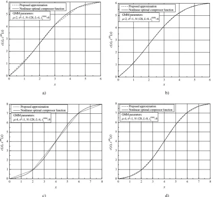
The numerical results are also derived for the assumed GMM. The following figures show the results of the conducted analyses, where

μ = 2 ( GMM ≈6

L

x ) and μ = 4 ( GMM ≈8

L

x ). The

considered values for the number of quantization segments are L = 4 and L = 8, whereas the number of quantization levels is N=128. By observing Fig. 4, one can easily notice how close are the optimal compressor function, c(x), and the obtained piecewise linear optimal compressor function:

( )

opt

( )

,

opt

x c x

c = _i x∈

[

xi−1,xi

)

, i=1,...,L. (44)

An interesting conclusion that can be derived is that the mean values of the GMM components affect the final result of the linearization process. For given L and for lower mean values, for instance, μ = 2, the piecewise linear optimal compressor function is closer to the nonlinear optimal compressor function compared to the case where μ = 4. Obviously, smaller mean values result with closer GMM components, and, as a result, better approximation of the optimal compressor function is achieved. The fact that the linearization error is lower for closer GMM components also has the effect on the obtained signal quality after linearization. Table 2 gives the overview of obtained signal quality (SQNR) values before and after linearization. One can see that the difference in SQNR values before and after linearization is smaller in the case of μ = 2, for each value of the number of segments. Also, as the number of quantization segments increases the difference in SQNR decreases.

5. Summary and conclusions

In this paper the novel method for designing the piecewise linear optimal compander (PLOC) has been proposed. The proposed method involves the mean-square approximation of the first derivative of the optimal compressor function. Optimization of the slopes of the linear functions, comprising the piecewise linear optimal compressor function, has been done by minimizing the mean-squared error introduced with the proposed approximation. By optimizing the slopes the number of uniform cells per segment has been determined. The analysis have shown that the piecewise linear optimal compressor function after optimization have slopes equal to the corresponding ones of the first degree spline approximation of the optimal compressor function. The designing of the PLOC has been conducted for the signals modeled with the Gaussian PDF and signals modeled with the GMM. It has been highlighted that the main contribution of the proposed

Table 1. Values of SQNRfor the proposed piecewise linear optimal compander

N SQNR [dB] (Approximation included) SQNR [dB] (By definition) 2L = 4 2L = 8 2L = 16 2L = 4 2L = 8 2L = 16

32 25.32 25.67 25.76 25.53 25.89 25.96

64 31.04 31.61 31.77 31.12 31.72 31.84

128 36.74 37.52 37.75 36.78 37.57 37.79

0 1 2 3 4 5 6 0

1 2 3 4 5 6

GMM parameters:

µ=2, σ2

=1, N=128, L=4, xGMM

L =6

c

(

x

),

c

opt

(

x

)

x

Proposed approximation Nonlinear optimal compressor function

0 1 2 3 4 5 6

0 1 2 3 4 5 6

GMM parameters:

µ=2, σ2

=1, N=128, L=8, xGMM

L =6

Proposed approximation Nonlinear optimal compressor function

c

(

x

),

c

opt

(

x

)

x

a) b)

0 1 2 3 4 5 6 7 8

0 1 2 3 4 5 6 7 8

GMM parameters:

µ=4, σ2

=1, N=128, L=4, xGMM

L =8

Proposed approximation Nonlinear optimal compressor function

c

(

x

),

c

opt (

x

)

x

0 1 2 3 4 5 6 7 8

0 1 2 3 4 5 6 7 8

Proposed approximation Nonlinear optimal compressor function GMM parameters:

µ=4, σ2

=1, N=128, L=8, xGMM

L =8

c

(

x

),

c

opt

(

x

)

x

c) d)

Figure 4. Optimal compressor function before and after piecewise linearization with the proposed approximation method for different combinations of GMM parameters

Table 2. Values of SQNRfor the proposed PLOC, for N = 128 and different GMM parameters SQNR [dB] (μ=2, GMM ≈6

L

x ) SQNR [dB] (μ=4, GMM ≈8

L

x )

L Before linearization After linearization Before linearization After linearization

2 33.36 dB 31.89 dB 31.9 dB 28.71 dB

4 33.36 dB 32.92 dB 31.9 dB 30.82 dB

8 33.36 dB 33.24 dB 31.9 dB 31.6 dB

design method is in simpler hardware and software realization of the PLOC compared to the nonlinear optimal compander. Analysis of the numerical results has lead to the conclusion that in the whole range of observed bit rates the proposed PLOC represents an effective solution for achieving higher signal quality (higher SQNR) in comparison to the uniform quantizer. In addition, it has been shown that the proposed PLOC processes the signal leaving its quality very close to the quality of the signal

processed with the optimal compander. The

applicability of the proposed quantizer for speech and

other signals modeled by Gaussian PDF and GMM recommends it for integration in A/D converters.

Acknowledgments

References

[1] A. Gersho, R. M. Gray. Vector Quantization and

Signal Compression. Kluwer Academic Publishers:

Boston, 1992, 133–172.

[2] A. Thompson, D. Emerson, F. Schwab. Conve-nient formulas for quantization efficiency. Radio

Science, 2007, Vol. 42.

[3] D. Kazakos, K. Makki. Robust companders. In:

Proceedings of the 6th WSEAS International

Conference on Telecommunications and Informatics,

Dallas (Texas), 2007, pp. 32–35.

[4] G. Bucci, M. Faccio, C. Landi. New ADC with piecewise linear characteristic: case study-implementation of a smart humidity sensor. IEEE

Trans. Instrum. Meas., 2000, Vol .49, No. 6,

1154-1166.

[5] J. Max. Quantizing for minimum distortion. IRE,

Trans. Inform Theory, 1960, Vol. IT-6, 7–12.

[6] J. Nikolić, Z. Perić, D. Antić, A. Jovanović, D. Denić. Low complex forward adaptive loss compression algorithm and its aplication in speech coding. Journal of Electrical Engineering, 2011, Vol. 62, No. 1, 19–24.

[7] J. Nikolić, Z. Perić, A. Jovanović, D. Antić. Design of forward adaptive piecewise uniform scalar quantizer with optimized reproduction level distribution per segments. Electronics and Electrical

Engineering, 2012, Vol. 119, No. 3, 19-22.

[8] J. Nikolić, Z. Perić, L. Velimirović. Simple solu-tion for designing the piecewise linear scalar

companding quantizer for Gaussian source.

Radioengineering, 2013, Vol. 22, No. 1, 194-199.

[9] L. Yang, D. Wu. Adaptive quantization using piecewise companding and scaling for gaussian mixture. Journal of Visual Communication and Image

Representation, 2012,Vol. 23, No. 7, 959-971.

[10] L. Velimirović, Z. Perić, J. Nikolić. Design of novel piecewise uniform scalar quantizer for gaussian memoryless source. Radio Science, 2012, Vol.47, RS2005.

[11] N. S. Jayant, P. Noll. Digital coding of waveforms,

principles and applications to speech and video.

Prentice Hall: New Jersey, 1984, 115-251.

[12] S. Na. Asymptotic formulas for variance-mismatched fixed-rate scalar quantization of a Gaussian source.

IEEE Trans. Signal Processing, 2011, Vol. 59, No. 5,

2437–2441.

[13] S. Na, D. L. Neuhoff. On the support of MSE-optimal, fixed-rate, scalar quantizers. IEEE Trans. Inf. Theory, 2001, Vol.47, No. 7, 2972–2982.

[14] W. Cheney, D. Kincaid. Numerical Mathematics

and Computing, Sixth edition. Thomson

Brooks/Cole, Belmont: USA, 2008, 371-425. [15] Z. Perić, J. Nikolić, A. Mosić, S. Panić. A

switched-adaptive quantization technique using μ-law quantizers. Information Technology and Control, 2010, Vol. 39, No. 4, 317–320.

[16] Z. Perić, J. Nikolić, Z. Eskić, S. Krstić, N. Marković. Design of novel scalar quantizer model for gaussian source. Information Technology and

Control, 2008, Vol. 37, No. 4, 321–325.