Reconfiguration for Multi Camera
Networks
Krishna Reddy Konda
Advisor: Dr Nicola Conci
The large availability of different types of cameras and lenses, together with
the reduction in price of video sensors, has contributed to a widespread use
of video surveillance systems, which have become a widely adopted tool to
enforce security and safety, in detecting and preventing crimes and
danger-ous events. The possibility for personalization of such systems is generally
very high, letting the user customize the sensing infrastructure, and
de-ploying ad-hoc solutions based on the current needs, by choosing the type
and number of sensors, as well as by adjusting the different camera
pa-rameters, as field-of-view, resolution and in case of active PTZ cameras
pan,tilt and zoom. Further there is also a possibility of event driven
auto-matic realignment of camera network to better observe the occurring event.
Given the above mentioned possibilities, there are two objectives of this
doc-toral study. First objective consists of proposal of a state of the art camera
placement and static reconfiguration algorithm and secondly we present a
distributive, co-operative and dynamic camera reconfiguration algorithm for
a network of cameras. Camera placement and user driven reconfiguration
algorithm is based realistic virtual modelling of a given environment using
particle swarm optimization. A real time camera reconfiguration algorithm
which relies on motion entropy metric extracted from the H.264 compressed
stream acquired by the camera is also presented.
Buddha-1 Introduction 1
1.1 Video based surveillance . . . 1
1.2 Camera planning . . . 3
1.3 Camera reconfiguration . . . 5
1.4 The solution . . . 7
1.4.1 Camera placement and static reconfiguration . . . . 7
1.4.2 Dyanamic reconfiguration . . . 10
1.5 Thesis organization . . . 11
2 Camera Planning 13 2.1 State of the art . . . 13
2.2 2D modelling . . . 18
2.2.1 Global and Local Coverage . . . 19
2.2.2 Camera Model . . . 21
2.2.3 Assumptions . . . 21
2.3 3D modelling . . . 25
2.3.1 Contribution . . . 26
2.3.2 Metrics for visual quality assessment . . . 28
2.3.3 Problem formulation and implementation . . . 34
2.3.4 Particle swarm optimization . . . 36
2.3.5 Algorithm and implementation . . . 36
2.4.2 3D model evaluation . . . 47
3 Light planning 73 3.1 State of the art . . . 73
3.2 Illumination and environment Models . . . 75
3.2.1 Illumination model . . . 75
3.2.2 Environment model . . . 76
3.3 Proposed algorithm . . . 76
3.3.1 Entropy calculation . . . 77
3.3.2 Particle Swarm Optimization . . . 78
3.3.3 Algorithm . . . 78
3.4 Testing and results . . . 79
4 Video Analytics 83 4.1 State of the art . . . 83
4.1.1 MPEG . . . 84
4.1.2 H.264 . . . 84
4.2 Motion descriptors . . . 86
4.2.1 Motion entropy measure . . . 88
4.3 Object detection and segmentation . . . 90
4.3.1 Algorithm . . . 90
4.3.2 Tuning the variance . . . 91
4.4 Fall detection . . . 93
4.4.1 Proposed method . . . 93
4.4.2 Algorithm . . . 95
4.5 Results . . . 96
4.5.1 Video segmentation . . . 96
5.1 State of the art . . . 105
5.2 Static reconfiguration . . . 106
5.3 Dynamic reconfiguration . . . 107
5.3.1 Area metric . . . 108
5.3.2 Camera network architecture . . . 109
5.3.3 Camera network and operation . . . 111
5.4 Validation . . . 113
5.4.1 Fall detection . . . 113
5.4.2 Entropy based reconfiguration . . . 115
5.4.3 Algorithm evaluation . . . 117
6 Conclusion 123
7 Publications 127
2.1 Target coverage for Map 1. . . 44
2.2 Target coverage for Map 2. . . 44
2.3 Target coverage for Map 3. . . 47
2.4 Entropy and focal length of images . . . 53
2.5 Distortion and location of spheres . . . 54
2.6 Environment radiometric constants . . . 55
2.7 Map1: Entropy and distortion after the initial setup. . . . 55
2.8 Map1: entropy and distortion after reconfiguration 1 . . . 57
2.9 Map1: entropy and distortion after reconfiguration 2. . . . 58
2.10 Map2: entropy and distortion after the initial setup. . . 60
2.11 Map2: entropy and distortion after reconfiguration 1. . . . 60
2.12 Map2: entropy and distortion after reconfiguration 2. . . . 61
2.13 Entropy and Distortion for Map2 Initial Setup . . . 61
2.14 Entropy and Distortion for Map1 after Reconfiguration 1 . 63 2.15 Entropy and Distortion for Map1 after Reconfiguration 1 . 63 2.16 Mean and variance of entropy across the frames. . . 69
2.17 Comparison for the HOG person detector. GT refers to the ground truth, P1 and P2 report the number of detections for the two subjects, respectively, and FP reports the number of false detections. . . 69
2.18 Number of STIPs obtained. . . 70
3.3 Results. . . 81 3.4 Light Power in watts. . . 81
1.1 A typical surveillance split screen . . . 4 1.2 Overview of the proposed system . . . 7
2.1 Pixel Mapping of Grid. Each area of the floor plan is cap-tured by a number of pixels that depends on the distance
from the camera. . . 19 2.2 Quality of view. The optimal distance for observation
de-pends on the objects of interest for the specific scene. . . . 21 2.3 Ray projection on to the environment from focal point . . 27 2.4 Images captured under different light exposure and
corre-sponding histograms: under exposed (left), correctly
ex-posed (center), and over exex-posed (right). . . 30 2.5 Example showing different levels of perspective distortion as
captured by the camera. . . 31 2.6 Projection of the area of interest on the image plane, to
lengths. . . 52 2.14 Images obtained at different focal lengths. . . 53 2.15 Sample image and distortion zones. Distortion is defined
according to Eq. (2.10). Colors corresponds to different levels of distortion: red correspond to µD > 0.8, orange
0.8 > µD > 0.5, yellow 0.5 > µD > 0.2, and green 0.2 >
µD > 0 . . . 54
2.16 Map1: total coverage map after initial placement (a),
recon-figuration 1 (b), and 2 (c). . . 56 2.17 Map1: snapshots from four cameras. . . 56 2.18 Map1: snapshots from the three cameras after
reconfigura-tion 1. . . 57 2.19 Map1: snapshots from two cameras after reconfiguration 2. 58 2.20 Map2: total coverage map after initial positioning (a),
re-configurations 1 (b) and 2 (c). . . 59 2.21 Map2. snapshots from four cameras . . . 59 2.22 Map2: snapshots from three cameras after reconfiguration 1. 60 2.23 Map2: snapshots from two cameras after reconfiguration 2. 61 2.24 Snapshots from four Cameras after initial placement . . . . 62 2.25 Map3: total coverage map after initial positioning (a),
re-configurations 1 (b) and 2 (c). . . 62 2.26 Snapshots from three Cameras after Reconfiguration 1 . . 63 2.27 Snapshots from three Cameras after Reconfiguration 2 . . 64 2.28 Panorama view of the test site. . . 64 2.29 Panorama view of the test site as seen in the virtual
tions of this setup are evident, as a large part of the images
refer to non-relevant areas of the environment . . . 66 2.31 Snapshots taken from the cameras positioned and configured
according to our optimization algorithm. The attention is now concentrated on the ground floor, where relevant
activ-ities are more likely to occur. . . 66 2.32 Total coverage map for the test site. . . 67 2.33 Plots reporting the difference in terms entropy variations
for the unplanned and planned configurations. A zoomed segment from frame 1000 to frame 2000 is also shown in the last two plots. For the sake of visualization, the mean value
of entropy has been subtracted from each sample. . . 71
3.1 Example of a light source (a), and of the environment (b)
generated using the POV ray tracing software. . . 76 3.2 Snapshots from two cameras after Light placement . . . . 81 3.3 Snapshots from two cameras Equidistant placement . . . . 82
4.1 Motion vectors extracted from a frame of the standard video sequence Stefan. The red arrows highlight the regions in
which the motion field exhibits strong disorder. . . 87 4.2 X axis represents variation of tuning factor M, mean of OX
and OY is multiplied by M and then squared to get σX2 and
σ2Y respectively . . . 92 4.3 (a) Velocity of the centroid of the person per frame. (b)
Variation of entropy and the events as marked using ground
erence method [43] . . . 97 4.6 Results obtained for a set of standard benchmarking
se-quences 1. . . 99 4.7 Results obtained for a set of standard benchmarking
se-quences 2. . . 100 4.8 Samples taken from the i-Lids dataset. . . 101
5.1 Segmented set of objects projected onto the environment
using the camera model and current parameters. . . 108 5.2 Target mode operation of the camera. . . 110 5.3 Various stages in transition of cameras from global to target
mode. . . 111 5.4 Reconfiguration of the camera carried out to guarantee full
visibility of the subject of interest. . . 114 5.5 Fall detection and subsequent reconfiguration of the camera
for better view. . . 119 5.6 Variation of entropy metric with movement of people. . . . 120 5.7 Global mode configurations of Camera 1 and Camera 2. . . 120 5.8 Path followed by people with respect images shown in
Fig-ures. 5.9 and 5.10. . . 120 5.9 Camera 1 switches to target mode; as the target moves out
of range, it transits back to global mode. . . 121 5.10 Camera 2 switches to target mode; as the target moves out
Introduction
In this chapter we introduce the history and various applications
associ-ated with video based surveillance. After the introduction we present the
relevancy of camera placement and reconfiguration for video surveillance
systems. A brief overview of the research in the area of camera placement
and configuration is presented. Brief introduction of the proposed solution
and its innovative aspects are also discussed.
1.1
Video based surveillance
The development of reel-to-reel media enabled the recording of surveillance footage. These systems required magnetic tapes to be changed manually, which was a time consuming, expensive and unreliable process, with the operator having to manually thread the tape from the tape reel through the recorder onto an empty take-up reel. Due to these shortcomings, video surveillance was not widespread. VCR technology became available in the 1970s, making it easier to record and erase information, and use of video surveillance became more common. Development of digital video compres-sion and advancement in storage technology using semiconductor devices has made video storage quite inexpensive. Owing to this fact surveillance footage up to a month is being stored in most of the deployed systems. Dig-ital video is generally recorded in one of the video compression standards formulated by ITU-T.Most of the present day data is stored in H.264 [70] compressed format. Video based surveillance is used in many areas of application of which we list out few of the important.
Crime prevention An analysis published by researchers from Northeastern
University and Cambridge University in 2009, discusses the impact of video surveillance on crime rate under various scenarios [69]. There was up to 51 percent decrease in crime rate in parking lots, up to 23 percent decrease in case of public transport system and up to 7 percent in general public spaces. As we can see from the study, video surveillance helps in crime reduction just by deployment of the system. There is also a possibility of surveillance footage giving us the evidence for any form of the crime that has been committed.
Industrial process Continual monitoring of work environment is essential
dangerous chemical substances are required to install video surveillance under the mandate of the law.
Critical area monitoring As a part of day to day life and also some
admin-istrative duties, there are certain critical situations and tasks where there will be utmost need for caution and transparency. Some of the situations include critical areas in defence establishments, which house technologi-cal know how of the systems, and also crititechnologi-cal financial transactions in banks and economic establishments. These kind of areas require round the clock surveillance by the stakeholders. Video surveillance is highly helpful in such situations. Markets and banks use constant video surveillance to overcome these issues.
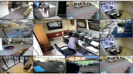
A typical surveillance monitoring split screen after the deployment of cameras in commercial establishment looks like as in Fig.1.1. Given the variety and the complexity of environment and video feed from various cameras, there is a definite need for intelligent and collaborative framework to address the deployment, data gathering and summarization of the video streams from various cameras.
1.2
Camera planning
consider-Figure 1.1: A typical surveillance split screen
furni-ture, equipment, and illumination systems. Furthermore, automatic tools can be designed so as to take into account additional constraints, such as the presence of obstacles, areas that are more difficult to reach with cables, areas subject to privacy constraints etc.
1.3
Camera reconfiguration
to satisfy specific coverage requirements, tremendously increases the flexi-bility of the network. The freedom to change the camera pan and tilt also after the physical deployment, may also help in simplifying the topology of the network, since with a reduced number of devices capable of being re-configured, it is possible to satisfy the requirements in coverage that would otherwise imply the use of a large number of static cameras to perform the same task. PTZ cameras can also be utilized to design an intelligent dis-tributed smart camera network, in which information is shared between the cameras in order to perform collective tasks like reconfiguration, detection and tracking. These aspects do not only increase the monitoring capabili-ties of the network, but they also contribute to a better observation of the events that take place in the area, as a reconfigurable camera system can be utilized to track moving objects by continuously changing the camera parameters according to the rules defined by the system architecture.
1.4
The solution
There are two principal objectives of this doctoral study. One of the ob-jectives is to propose a novel, low complexity camera placement and static re-configuration algorithm for multi camera network and the other is to propose a generic, smart, distributive,low complexity and dynamic recon-figuration algorithm based on video analytics of the events that occur in deployed environment.Overview of the system that we propose to develop is shown in Fig.1.2
Figure 1.2: Overview of the proposed system
1.4.1 Camera placement and static reconfiguration
into account the static or long term changes that occur in the environments. Examples are camera malfunction and occlusions.
The Research in this areas is broadly classified into three categories.
• Generate and Test Approach: In Generate and Test approaches all the constraints and models are incorporated into a test simulation model and solution is obtained by evaluating all possible configurations.
• Synthesis Approach: In case of synthesis approach we model the given constraints as analytic functions. Despite being the most popular ap-proach of the three, the task is somewhat complicated as it involves so many parameters, and modelling a constraint in such high dimen-sional space is difficult. In this approach various models are used to describe different constraints, and then these models are solved for various camera parameters using iterative solutions.
• Expert Systems: The Expert Systems approach addresses the high-level aspects of the problem in which a particular viewing and illumi-nation technique is chosen from a set of previous data which has been accumulated over time. For instance, whether front or back illumi-nation is more appropriate for the particular object and the features to be observed. An expert system is primarily used for advice for a certain set of tasks.
expert systems. We want to model the aspects that are to be optimized as analytic functions as is the case of synthesis approach. Similarly, we would like to optimize the coverage by generating and simulating the camera net-work response to the environment using virtual modelling technique, which is in line with ’generate and test approach’.
Innovative aspects In general most of the present day camera planning
al-gorithms, concentrate on coverage maximization with a simplistic camera model which has uniform coverage and also assume uniform lighting. How-ever we feel that such a description of the problem is an oversimplification. The innovative aspects of our approach are listed below.
1. Camera model We propose a three dimensional, realistic and innova-tive camera model based on ray projection, with number of rays being proportional to the resolution of the camera. Such a representation allows us to measure the coverage in terms of pixel density.
2. Distortion modelling Optimization is also focused on minimizing per-spective distortion as seen by the camera, made possible by the ray projection camera model.
3. Environment model We also model the environment to its slightest detail using modelling parameters like colour, texture, reflection coef-ficient, and diffusion coefficient using POVray software [50]
4. Light modelling We model the light sources, often ignored in coverage maximization problem. There is a possibility of modelling an array of light models like circular, area, parallel etc. The attenuation rate of light is also modelled based on the environment.
to get best possible views for the cameras. As the entropy or quality of view is highly dependent on illumination and focal length of the camera.
1.4.2 Dyanamic reconfiguration
Dynamic reconfiguration algorithm for the camera network helps in reduc-ing the cost and also improvreduc-ing the efficiency of the system as discussed in Section 1.3. The requirements of the algorithm are as follows
1. Real time operability Any dynamic system requires a real time re-sponse, hence we need propose a real time video event detection and information gathering algorithm. Which also requires low bandwidth requirement in order to avoid delays.
2. Distributive algorithm We intend to propose a solution which is ro-bust to sensor failures, hence the algorithm needs to be distributive. Distributive architecture can also be easily implemented using net-work of low power embedded devices rather than a high complexity centralized computational unit.
3. Generic Since the video surveillance systems are deployed for variety of applications, the solution should be as general as possible. Hence the reconfiguration algorithm should not be biased towards any par-ticular surveillance application.
Innovative aspects Apart from being distributive, low complexity and generic,
the algorithm has following innovative aspects.
video stream. This reduces the complexity as there is no feature ex-traction, which is generally computationally very intensive. Com-pressed stream also brings down the bandwidth requirement.
2. Motion entropy In this thesis we propose a generic quantitative mea-sure for information in video directly derived from compressed video bit stream. It will be the basis of the camera reconfiguration and cam-era handoff. This metric can be used in many ways to achieve various computer vision tasks like tracking, segmentation, anomaly detection etc.
3. Scalability The Proposed algorithm is robust to sensor malfunction and is easily scalable to any number of cameras without any further addition of infrastructure or hardware.
4. Customizability Although proposed system is generic and is not biased towards any computer vision application. User can easily train the system to achieve desired result in many computer vision application areas.
5. Deployment Algorithm relies on motion field as a basis for many of the derived metrics. Which is extracted from the compressed bit stream. Owing to the low complexity, the algorithm can be easily embedded in the video encoder platform inside the camera hardware thereby eliminating any requirement of additional hardware.
1.5
Thesis organization
Camera Planning
In this chapter we discuss about the camera planning and static
reconfigu-ration. In order to serve various surveillance environments, both 2D and
3D camera planning models are presented. 2D model is more suited for
large environments and is of less complexity, whereas 3D model is more
accurate and is suited for complex indoor environments.
As discussed in the previous chapter, most of the algorithms in the state of the art consider camera planning as a simplistic coverage maximization problem. Camera models used are also uniform and fixed, such an assump-tion is highly over simplistic. Further such a model would be only valid for static cameras. Rendering these algorithms inapplicable for PTZ cam-eras which are increasingly replacing the static camcam-eras. Many of other critical parameters like lighting and other radiometric properties are also overlooked. As a solution to these problems we present two camera models for planning based on the size of environment.
2.1
State of the art
challenges. In this section we will briefly introduce how the problem of coverage maximization has been faced in literature, presenting the most important milestones in this research area.
A very simple model to describe the problem of coverage maximization is the so-called art gallery problem (AGP), where the minimum number of guards is to be determined for a given area [12]. A variant of the AGP is known as the Watchmen Tour Problem (WTP), where guards are allowed to move inside the area perimeter [7]. The objective in this case is to determine the optimal number of guards and their route to guarantee the detection of an intruder with an unknown initial position. Both approaches can be useful to understand the problem, but are generally not suitable for the application in real-world scenarios, when a real deployment of sensors is required. Therefore, more sophisticated algorithms have to be adopted to take into account the most important elements of the surrounding world, which include constraints on observability [62], but also camera parameters (field of view, focal length), and illumination parameters.
The HEAVEN system by Sakane et al [59] was proposed with the goal of modeling the coverage exploiting a simulation tool. HEAVEN uses a spherical representation to model the sensor configuration. To this aim, a geodesic dome is created around the object, tessellating the sphere with an icosahedron that is further subdivided in a hierarchical fashion by re-cursively splitting each triangular face into four new faces. This process can be implemented at different levels of detail, depending on the available computational resources. The viewing sphere is centered on the object and its radius is equal to a distance (chosen a priori) from the sensor to the target object.
pro-cess typically turns out to be more complex as it involves many parameters, resulting in a high-dimensionality space, in which the optimization has to be performed. Nevertheless, and in case the computational cost is not the first priority, modeling constraints as analytic functions can bring some advantages. In fact, each requirement generates a geometric constraint, which in turn is satisfied in a domain of admissible locations in the three-dimensional space. The set of locations generated by each constraint can then be intersected in order to determine the ones that best satisfy all con-straints simultaneously. An early work in this area is proposed by Cowan et al [13], in which camera locations are generated also with respect to illumination planning.
A considerable portion of the present day research is carried out fol-lowing these principles, also thanks to the ever-increasing available com-putational power, different models can be defined for the relevant camera parameters using iterative solutions. For example in [21] Erdem et al pro-pose a camera positioning algorithm based on a binary optimization tech-nique and using polygonal spaces presented as occupancy grids. Bodor et al [5] propose an algorithm to optimize views so as to provide the highest resolution of objects and motion in the scene.
dis-cusses how an iterative approach can be used to solve a complex problem like camera positioning, stressing the fact that also for a limited number of cameras, hundreds of thousands of configurations are possible. Similarly, Song et al [63] describe a generalized framework for multi-camera tracking using the Kalman consensus algorithm, along with reconfiguration using game theory approaches.
In the work by liu et al [37] the authors propose a generalized statis-tical framework for optimal deployment of large scale camera networks. Although the proposed solution is evaluated in a simulated environment it gives another perspective of the deployment problem, especially with respect to large camera networks with special focus on user constraints. Similarly in [41] authors propose a camera view quality criteria based on application specific and environment specific functions However the algo-rithm is targeted at quality of view rather than for coverage. In [11] Cheng et al try to optimize the visual sensor networks with respect to the barri-ers encountered in the coverage, however this is yet another paper which addresses the optimization problem in application specific sense. State of the art in this area is quite rich with lot of works evaluating the problem in many unique perspectives, however there are many glaring deficiencies which render most of the algorithms inapplicable in real scenario. The deficiencies are summarized below.
common, which have many configurations for a given location.
2. Light Modelling All the works in this area assume uniform illumina-tion. Such an approximation might as well be valid during the day, but is not at all acceptable during the night. Illumination is one of the most critical aspects of any video surveillance system, as it has dra-matic impact on accuracy and performance of most video processing and computer vision algorithms. Hence for a successful deployment of the surveillance system a proper estimation of lighting is absolutely necessary.
3. Simplistic environment model Most of the works represent the envi-ronment as a simple 2D map with lines representing objects or obsta-cles. Such an assumption is simply un viable as they cannot correctly describe the sensor response of the camera to that of the deployed environment. Thereby completely ignoring the qualitative aspect of the video that has to be recorded.
4. Distortion There are two types of distortions in a video, one is lens distortion while the other is perspective distortion. Lens distortion is easily rectified using interpolation and other techniques, however perspective distortion cannot be eliminated as it results from the view angle of the camera. None of the state of the art address this problem.
optimizing other parameters apart from location.
2.2
2D modelling
2.2.1 Global and Local Coverage
In order to model global coverage, we consider three conditions that need to be satisfied, namely pixel density, quality of view, and light intensity.
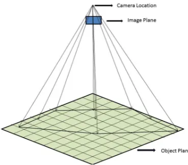
Pixel density refers to the fact that the information obtained from an image or a video is dependent on the number of pixels per surface area of the environment. Pixel density can be modelled as a function of the field-of-view and the resolution of the camera. In order to model the pixel density, we propose to represent the camera as a point source and each pixel of the CCD as the corresponding ray that emerges from the point source. Accordingly, far away areas in the environment receive less rays, corresponding to lower pixel density, whereas areas closer to the camera will be intersected by a higher number of rays, thus achieving higher resolution. An example about the mapping of the floor plan to the camera CCD is illustrated in Fig. 2.1.
Figure 2.1: Pixel Mapping of Grid. Each area of the floor plan is captured by a number of pixels that depends on the distance from the camera.
the recognition of an object will strongly depend on its distance from the camera: if it is too distant details will be unintelligible; if it is too close, the whole object might not be visible entirely due to limited field-of-view of the camera. To take into account this parameter, we model the vis-ibility constraint as a Gaussian distribution that is computed along the ray emerging from the camera. Fig. 2.2 shows the visibility of the object modeled a Gaussian distribution. The optimal distance is located at the center of the Gaussian, and needs to be specified according to the size of the objects to be monitored (human, cars, etc.).
The light intensity at the object location will also affect quality of the captured image, and it is therefore a very important parameter to be in-cluded in the model. According to the standard decay of the light intensity, we model it as an inverse square function of the distance from the light source. This model is not exhaustive for illumination modeling, since it does not take into account for example, of reflections and shadows. The term is meant to model the light intensity of specific spots in the envi-ronment, so as to change the cameras positioning also according to this parameter.
As far as the local coverage is concerned, each area of interest (doors, windows, statues, paintings, other objects, etc.) is modeled as a Gaussian function of distance from the camera. The mean of the Gaussian defines the optimal distance of the specific target from the camera, namely where the quality of view for that particular target is maximum. This value is related to the size of the target as well as its relevance in the scene. We have also planned to include light intensity as a parameter in target coverage, measuring the expected intensity of light at the target location. For instance, if a target falls under an area of low light intensity, the camera has to be placed closer to it.
Figure 2.2: Quality of view. The optimal distance for observation depends on the objects of interest for the specific scene.
elements are provided in next sections.
2.2.2 Camera Model
The parameterization of the camera model, as discussed above, includes the three aspects of pixel density, quality of view, and illumination.
2.2.3 Assumptions
only require the definition of an additional constraint.
Equations and Constants
As we have pointed out in the previous section, the quality of view of an object is modeled as a Gaussian distribution positioned along the ray emerging for each pixel of the camera, as given in Eq. 2.1
Q(di) =
1
√
2πσexp
−(di−D
opt)2
2σ2
(2.1)
where di is the distance of the cell on the i-th ray hitting it, and Dopt is
the optimum distance at which the object has maximum quality of view. In the current scenario Dopt is chosen as a constant, which depends on the application and varies on the purpose of camera deployment.
The second term we need to define is related to the information about the light intensity at a given location, defined as in Eq. 2.2
L(dj) =
P
d2j (2.2)
where P is the power of the j-th light source with j ∈ {1. . . S}, and dj
is the distance of the point from the light source. As for the local coverage, the model is in Eq. 2.3:
Tk = exp
− (dk −D
opt k )
2
2σd2
k ∗
S0 P
j
L(dj)
(2.3)
where dk is the distance of the k-th target from the Nearest Visible
camera, σdk is the variance of the target coverage, and D
opt
k is the optimum
distance from camera for the k-th target where the quality of view is max-imum. Ldj is the light intensity at the target location given by summation
While calculating the contribution of each light source, blockage of light due to the presence of obstacles is also taken into account. Smaller values for σdk will keep the cameras strongly focused on the targets, while higher
values for σdk will relax the constraint, accepting targets to be also
decen-tralized in the field-of-view of the camera. The parameter is in general related to the environment size, as well as to the coverage requirements.
In order to determine the areas that are visible in the map, we have to fix a threshold for visibility for the quality of view function. This threshold is calculated in accordance with [20]. According to the standard 100 Lu-mens is the required amount of light for casual observance of surroundings. Lumens is a SI derived unit for the luminous flux, which is different from radiant flux as it also takes into consideration human eye sensitivity. Now we classify a given cell in a grid to be covered if and only if the total lumi-nous flux in the cell is at least 100 Lumens, and the total quality of view as defined by summation ofQ(di) of individual rays that pass through cell,
is at least 0.5. Since the scale used here is 4 pixels per meter, 100 Lumens corresponds to 1 watt per square meter according to most commercial light manufacturers [1].
Algorithm
The proposed algorithm can be described in five steps, as explained here after.
Step 2 - Calculate Global coverage. In order to calculate the global cov-erage, the environment map is divided into a grid of N xN pixels. The granularity of the grid is chosen depending on the map scale, as well as on the accuracy in positioning that we want to achieve. The finer the grid, the more accurate will be the result, at a cost of a higher computational complexity. For each camera, the number of rays that pass through each cell of the grid are computed. While estimating the number of rays, ob-structions caused by the obstacles are also taken into account. The higher the number of rays that cover a grid cell, the higher the pixel density, as calculated in Eq. 2.4:
C(m, n) =
R
X
i=0
Q(di)∗ S
X
j=0
L(dj) (2.4)
where C(m, n) is the final quality of view metric obtained for a specific cell, while m and n give the location of the cell in the map. As we can see from Eq. 2.4, this metric will weight the quality of view function measured as in Eq. 2.1 considering the number of rays that intersect the cell (R). Conversely, we can say that the number of pixels occupied by a particular cell in the video frame is directly proportional to the number of rays that pass through that cell in the grid. The light intensity component is instead obtained by summing up the contributions of all light sources in that point (S).
We then label the cell as “visible” only if the quality of view is higher than a predefined threshold, fixed in accordance with a recommendation from the European standard for lighting levels based on activity [20]. The global coverage is estimated as the number of visible cells divided by total number cells in the grid (Eq. 2.5).
CG =
Cellsvisible
Cellstotal
Step 3 - Include Local coverage. For a given camera position the local coverage is given by Eq. 2.3. Accordingly, overall local coverage is given by Eq. 2.6:
CT =
1 T
T
X
k=0
Tk (2.6)
where T is the total number of target objects.
Step 4 - Fitness Function. We need now to define a fitness function that will be used by the PSO algorithm as a target for the optimization. The proposed fitness function combines both global and local coverage, and each term can be weighted according to the users’ preferences and the application requirements (Eq. 2.7).
F(CG, CT) = (1−CG)∗w + (1−CT)∗(1−w) (2.7)
In Eq. 2.7 CG represents the global coverage and CT represents the
local (target) coverage; w is the weight assigned by the user to balance the tradeoff between global and local coverage. We can notice from Eq. 2.7 that, as soon as the global and local coverage approach 100%, the fitness function converges to zero.
Step 5 - PSO. PSO is applied to the solution space defined in Step 1. At each iteration, the particle position and velocity is updated, until conver-gence. Convergence is usually achieved when the fitness function reaches a minimum, or when a termination criterion is fulfilled (e.g., maximum number of iterations).
2.3
3D modelling
the camera and environment are paramount. This model includes many ad-ditional features like radiometric properties in terms of environment model. Camera model is based on classic pin-hole camera model and is completely replicated to obtain visual quality and perceived distortion.
2.3.1 Contribution
In this sub section we highlight the novel elements of our approach com-pared to the solutions available in the literature. They can be summarized into four distinctive features, as described in the next paragraphs.
Camera modeling
Most algorithms for camera networks planning use a model for the camera that does not take into account the sensitivity in terms of quality of the captured information. This is for example the case of surveillance systems, which goal is to implement efficient algorithms capable of recreating the human observation for event detection and analysis tasks. We propose a realistic camera model, which simulates the camera view, and assesses the visual quality for a given environment, by analyzing the scene in a virtual domain. The advantage of using a virtual representation enables a highly reliable evaluation of the camera configuration, providing a quantitative metric, both in terms of visual quality and coverage. Pictorial representa-tion of this ray projecrepresenta-tion camera model is shown in Fig.2.3
Illumination and radiometric properties
Figure 2.3: Ray projection on to the environment from focal point
the radiometric properties of the surfaces, namely their color and their reflection coefficient.
Distortion
Distortions can be introduced at different levels of the acquisition and pro-cessing stages. In particular, lens and perspective distortions are inherent in the captured videos, and can seriously affect the system performance, requiring image rectification. Such situations can be handled a priori, by selecting the configuration of the camera network that reveals the smallest level of distortion.
Scalability and user interaction
2.3.2 Metrics for visual quality assessment
Visual information
A good visibility of the observed scene is a fundamental step for a cor-rect application of automatic analysis tools. Therefore, while planning the camera configuration, several factors have to be taken into account. For example, one has to position the cameras so that the image sensors are exposed to the correct amount of light. Videos captured under good il-lumination conditions will require less pre-processing and maximize the gathered information. However, gauging directly the sensor response of the camera is not a viable option, since planning should be done before the actual positioning of the sensorial equipment in the environment. In our system we deploy the virtual cameras in the synthesized domain. We successively use the image generated by the virtual model to assess the sensor response for various camera configurations. Considering that our virtual model also includes the configuration of the light sources, such an approximation turns out to be particularly realistic.
In order to measure the amount of information present in the captured image we propose to start from the histogram of the image, by determining the bins distribution. In fact, in presence of an under exposed image, the histogram will be biased towards the lower levels, while for an over exposed image, the histogram will likely be biased towards the higher intensity levels.
In order to quantify the quantity of information in the image, we com-pute the entropy, a metric that has already demonstrated to be effective in measuring the quality of the captured image [27]. For a given configu-ration of the i-th camera, and the corresponding captured image Ii, with
i ∈ {1, . . . , N}, let the intensity levels be Ω = (l1 < l2 < . . . li· · · < lN),
H(Ω) =
n
X
pi∈Ω
−pilogpi (2.8)
In Eq. (2.8) pi is the normalized region under each intensity level li ∈ Ω,
considering that the entropy is directly proportional to the information content of the image. We then maximize the image information, given a solution space, which consists in our case of all possible combination of the camera position (X, Y, Z), pan, tilt, and zoom:
H(Ω)opt = argmax n
X
ri∈Ω
−pilogpi
!
(2.9)
where i represents a single instance of the solution space.
Instead of considering the standard RGB space, the analysis is carried out in the LAB color space, because of its property of being perceptually uniform, meaning that the same distance computed over different points of the color space, would correspond to an equal variation from a perceptual viewpoint.
Fig. 2.4 shows three sample images generated with our virtualization tool, at different levels of exposure, and the corresponding histogram dis-tributions.
Distortion
Figure 2.4: Images captured under different light exposure and corresponding histograms: under exposed (left), correctly exposed (center), and over exposed (right).
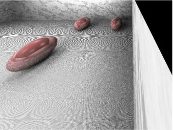
distortion is not uniform across the image, therefore while planning the camera network we have to make sure that the area of interest of a given environment falls under the portion of image, which exhibits the minimum amount of distortion. In Fig. 2.5 we show an example of the varying levels of distortion in an image. The image consists of three spheres positioned at different distances from the camera. All spheres have a radius of 0.5m. We can observe from the figure that the sphere in the left most part of the image is subject to severe distortion and appears like an ellipsoid with a large difference between the major axis and minor axis. The level of dis-tortion then progressively decreases, until, the sphere in the extreme right of the image preserves the original shape. It is clear from the observation that the camera should be positioned in such a manner that objects of interest is not distorted.
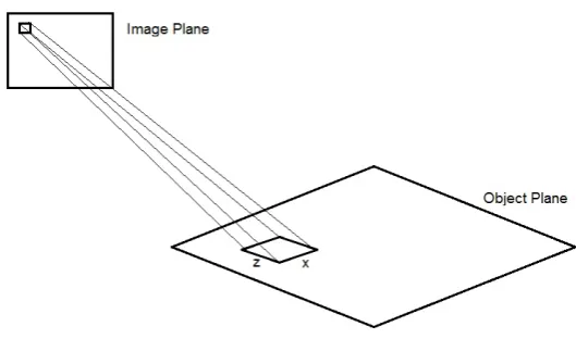
ideal scenario, this ratio should be equal to the aspect ratio of the image. In order to estimate the distribution of the distortion we need to compute the mean and variance across the projection of the image plane on the area of interest (Fig. 2.6). The mean value of the distortion D can be defined as:
µD =
1 Ai
∗
I
X(xi+dxi)−X(xi)
(Z(yi +dyi)−Z(yi))∗R
(2.10)
where Ai is the area of the entire image, xi and yi correspond to the
variations along X and Y on the 2D image plane, and R is the aspect ratio. In the discrete domain, the equation becomes:
µD =
1
(Nw−1)∗(Nh−1)
∗
Nw−1,Nh−1
X
i=1,j=1
X(i+ 1)−X(i) Z(i+ 1)−Z(i)
(2.11)
where Nw and Nh is the number of pixels in the horizontal and vertical
directions in the 2D image plane, respectively. Similarly, variance can be calculated as:
σD2 = 1
(Nw −1)∗(Nh−1)
∗
Nw−1,Nh−1
X
i=1,j=1
[X(i+ 1)−X(i)
Z(j+ 1)−Z(j) −µD]
2
(2.12)
After computing the mean and variance of the distortion, we can formu-late a suitable cost function, resulting as the configuration that minimizes both terms:
Figure 2.6: Projection of the area of interest on the image plane, to compute the distortion.
Coverage
With the term coverage, we refer to the portion of the environment visible by each camera. Coverage has been historically modeled through a fixed cone deriving from the field of view of the camera (2D or 3D), with uniform distribution of quality. We believe though that this assumption is too simplistic and may be valid only for very simple and static scenarios. In our case we present a model of the field of view, in which rays are projected from each pixel into the environment, thus assuming each pixel in the camera as a light emitter hitting a portion of the observed real world. Such a model should be as close as possible to the real world scenario, and allows tracking the changes in the distribution of ray projections according to the relative changes in the camera parameters. In order to compute the percentage of the area covered by each camera, the environment is divided into a grid of cells of equal square size. Each pixel is projected onto the real ground plane and classified as belonging to a specific cell. The cells, which have at least one ray intersecting them are classified as visible, and all others are considered invisible to the camera.
maximum spread in the distribution of rays, so as to maximize the number of visible cells. The number of rays intersecting the grid cell is a function of the cell location (X, Y, Z), focal length f, camera location x, y, z, pan θ and tilt φ:
Nrays(X, Y, Z) = F(X, Y, Z, x, y, z, φ, θ) (2.14)
Also in this case we can formulate a cost function for the area covered in terms of the number of cells, which at least have one pixel projection on them, normalized by the total number of cells. The maximization of this condition implies:
Covmax = argmax
Count(Nrays(X, Y, Z) >= 1)
Ncells
(2.15)
2.3.3 Problem formulation and implementation
As for the metrics described in the previous paragraphs, entropy and distor-tion are camera-specific and mutually exclusive, i.e, they do not influence one with each other. Coverage, instead, has to be calculated collectively.
Initially, we formulate the cost function for both entropy and distortion for each individual camera. Entropy, mean, and variance of distortion are described in Eq. (2.8), Eq. (2.11), and (2.12). In order to normalize the cost the equations can be expressed as:
Di = exp(−(µD +σD2 )) (2.16)
Ei = [1−exp(−H(Ω)i)] (2.17)
entropy and distortion are equally important in the cost function. Taking all these factors into account the formulation becomes:
Ci(Ei, Di) =
1 Nrays
∗[Di/2 +Ei/2] (2.18)
Let there be N cameras that have to be positioned in the environment, and let the area covered by each camera be defined as Ai for the i-th
camera. The total area covered by the network is given by:
[
∀i
Ai =
X
∀i
Ai −
X
i<j
Ai
\
Aj +....+ (−1)n+1
\
∀i
Ai (2.19)
which corresponds to the sum of the individual contributions in terms of coverage for the single cameras, minus the redundant area (overlap). Hence, our cost function should increase the overall visible area while min-imizing the overlap between cameras field-of-view, as shown in Eq. (2.20):
CV(∀i) =
1 Aenv ∗ " X ∀i
Ai −
X
i<j
Ai
\
Aj +...+ (−1)n+1
\
∀i
Ai
# (2.20)
where Aenv is the total area of the environment. Combining the global
coverage and individual camera measures we obtain the final cost function:
Cf inal = wtask(CV(∀i))+
(1−wtask)∗
" 1 N ∗(
N
X
i=0
Ci(Ei, Di))
#
(2.21)
2.3.4 Particle swarm optimization
Solving a problem involving six parameters describing the 3D geometry of the environment is a rather complex task, made even more critical due to the presence of random obstacles, and the use of traditional problem solving techniques like steepest descent is not a viable solution. Hence we propose to use a global optimization technique, namely the PSO, which has been already adopted in literature to solve camera planning problems [46] [74].
PSO [16], is a robust stochastic search technique based on the movement and intelligence of swarms. It has demonstrated to be effective in solving complex non-linear multidimensional discontinuous problems in a variety of fields [17]. Unlike other multiple-agent optimization procedures such as Genetic Algorithms (GA) [24], PSO is based on the cooperation among the agents rather than their competition. Three main advantages of the PSO over the GA can be identified. In the first place, PSO requires a reduced algorithmic complexity, since it considers only one simple operator, that is the particles velocity updating, while the GAs use three operators and the best configuration among several options of implementation needs to be chosen. Then, PSO parameters are easier to calibrate and to manip-ulate. Finally, PSO has a major ability to prevent the stagnation of the optimization process, thanks to a more significant level of control of its parameters [58] [18]. Further PSO has been widely used for coverage max-imization in visual sensor networks [25, 71, 73]. Further details about the optimization algorithm, can be found in the relevant literature [16] [17].
2.3.5 Algorithm and implementation
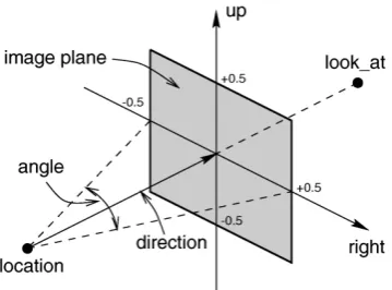
on the surface plane. The orientation of the image plane is defined by the pan and tilt of the camera (Fig. 2.7).
Figure 2.7: Model of the camera [50]
In order to measure the visual information (as described in Section 2.3.2), we need a virtual environment to simulate the camera view, vi-sualize and evaluate the obtained cameras position. For this purpose we use Persistence of Vision, or POV-Ray, a ray tracing software [50]. This software has a unique scene description language that can be used to repli-cate the objects in the real world, including their radiometric properties. Similarly, light sources can also be modeled, by specifying the attenuation along the travel distance. Matlab is then used to simulate the ray trac-ing and for image registration, starttrac-ing from the simulated camera views obtained from POV-Ray, using the geom3D library [35].
The proposed algorithm, consisting of five main steps, can be described through the pseudocode shown in algorithm 1. Similarly pseudo code for subsequent particle swarm optimization is given by algorithm 2.
information is then converted into the POV-ray scene description language and the PSO is initialized. At each iteration of the algorithm, the particles are updated based on the fitness function.
Step 2 - Calculate entropy and distortion. Camera views are generated using POV-ray and the values for entropy and distortion are evaluated to obtain the camera measure in Eq. (2.18).
Step 3 - Calculate global coverage. The global coverage can then be computed, also taking into account the overlapping areas among the cam-eras. As described in the previous section, the surface area of the object of interest is divided into a grid of cells of equal size, and the coverage measure is calculated as described in Eq. 2.15.
Step 4 - Calculate configuration cost. The values obtained for each camera are then combined according to Eq. (2.21), where user or task-specific adaptation is also taken into account.
Step 5 - PSO. The fitness function is updated and the set of particles in the swarm optimization are updated until the termination criterion is reached.
2.4
Evaluation
This section deals with testing and evaluation of both 2D and 3D cam-era planning models. Test scenarios and obtained results are extensively discussed.
2.4.1 2D model
input : Surface S of object of interest divided intoN ×M cells of equal size
input : Number of Cameras N C
input : Map I Description in POV-ray scene description language
input : Camera Resolution
output: Fitness Value
Initialize camera positions from PSO;
Initiate the number of rays for each camera based on the video resolution;
Generate camera view using POV-ray;
EOV ; % Quality of View of Cameras
DM ; % Mean of perspective distortion
DV ; % Variance of perspective distortion
goodCells= 0 ; % Number of cells with good coverage C = 0; % Obtained coverage for each cell
fori←1 to N do forj←1 to M do
fork←1toN C do
pixelDensity←RayIntersect(i, j, k); C(i, j) =C(i, j) +pixelDensity(k);
end
if C(i, j)>= 0 then
goodCells++ ;
end
if C(i, j)>1then
goodCells– ;
end
end
end
fork←1to N C do
EOV (k)←Entropyofview(k); DM(k)←Distortion_mean(k); DV (k)←Distortion_variance(k);
CM=CM+NormalizedRayIntersectCount(exp(−(DM(k) +DV(k)))/2 + (1− exp(−EOV(k))/2);
end
Cg ← goodCellsN∗M ; %Compute global coverage
%The final output is a combination of global coverage and camera measure with weight wG
F(CG,CM) ←1−[Cg∗wG+CM(1−wG)]; Return F(CG,CM);
input: Number of Particles
input: Number of Iterations
InitializeParticles;
for i←1 to Number of Iterations do
for j ←1 to Number of Particlesdo
F(j)= Fitness(j);
if F (j) <pBest(j)then
pBest(j) ←F(j);
end
end
gBest =min(pBest(j));
for j ←1 to Number of Particlesdo
CalculateVelocity(j);
UpdateVelocity(j);
end
end
Algorithm 2: Pseudocode of the PSO.
relevant in large environments with large number cameras. It offers a low complexity alternative with only a slight reduction accuracy.
Scenarios
opti-mum distance for quality of view is fixed at 40 pixels in the map, which corresponds to sbout 10 meters in the real environment.
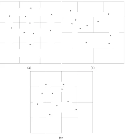
In order to assess the validity of our approach, we tested the algorithm on three different maps. As far as the simulation procedure is concerned, we initially determine the cameras position on the map, assuming that no object is present. This is equivalent to optimizing only with respect to global coverage.
After the initial setup, nine different objects of interest are placed in the map. At this point the algorithm is required to re-align the cameras, keep-ing the positionkeep-ing of the sensors fixed. This implies that in determinkeep-ing the new camera parameters, only local coverage is considered, thus setting w = 0.
The environment maps used for the testing are shown in Fig. 2.8. Cam-eras can be positioned along internal and perimeter walls of the environ-ment. In the picture we also show the positioning of the targets that will be introduced after the initial setup of the camera infrastructure is found.
Experimental Results
As explained in Section 2.4.1, we will present the results obtained in the selected scenarios by first illustrating the quality of the global coverage achieved in the initial positioning, and then focusing on reconfiguration for local (target) coverage.
Initial Positioning Initially, the environment in which the cameras have to
(a) (b)
(c)
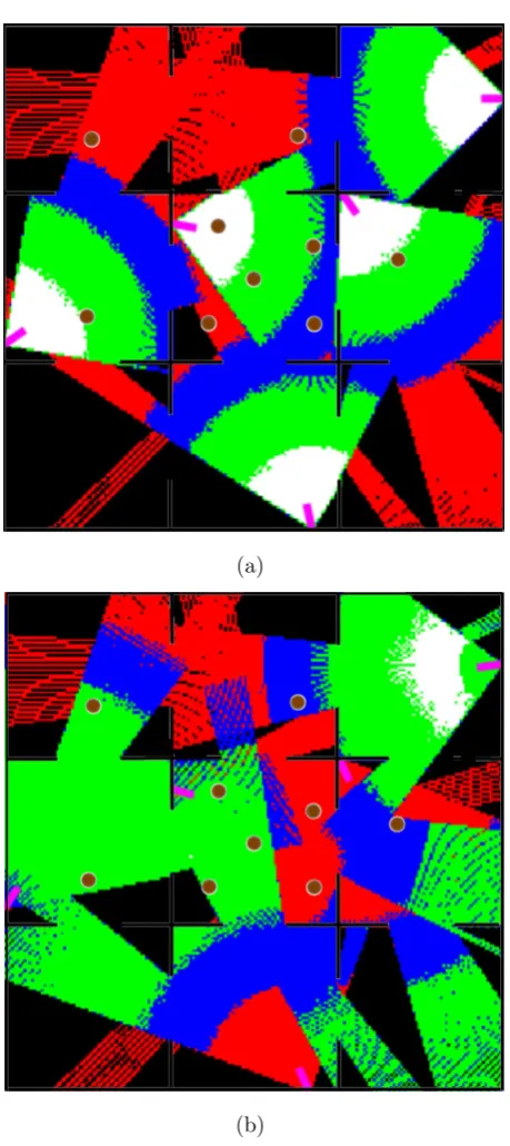
quality of the coverage in over the entire map. Areas which have maximum coverage (i.e. when C(m, n) is greater than 100) are represented in white, and areas which fall in the range 10 <= C(m, n) < 100 are represented in green. Blue indicates areas, which satisfy 0.5 <= C(m, n) < 10. Red areas represent zones of the environment, which are visible to cameras but fall below our visibility threshold of 0.5. Black areas are not visible to cameras due to the presence of obstacles.
Reconfiguration After the initial positioning is completed, 10 targets are
randomly distributed over the map. The goal of reconfiguration is to max-imize target coverage; however, in most surveillance scenarios camera de-ployment is fixed and does not allow repositioning after installation, unless PTZ cameras are used. Hence, according to our model the only recon-figurable parameters are pan and optical zoom. The algorithm is re-run considering the absolute position of the cameras fixed, thus optimizing target coverage.
Experiment 1 The input map to the algorithm is shown in Fig. 2.8(a). A
uniform illumination of 10 Lumens is considered, and the initial positioning is performed with Optical and Digital Zoom both set to 1x, while pan is a free parameter along with the x-z positions that can be adjusted to obtain maximum coverage.The coverage map after the initial placement of cameras is shown in Figure 2.9(a). After the Initial positioning of the cameras, nine random targets are distributed over the entire environment map as we can see from Figure 2.9(a) and Table 2.1 these targets are not covered properly. The results obtained are shown in Figure2.9(b)
Table 2.1: Target coverage for Map 1.
Configuration White Green Blue Red Black CT CG
Initial 0 2 0 7 1 0.3883 0.5015
Final 0 6 2 0 1 0.7443 0.4193
on local coverage. As can be seen from the figures in Table 2.1, CT has
increased both from quantitative and qualitative viewpoint. Initially only two targets were sufficiently covered but after realignment only one target has been left out and eight are covered. CG in turn signifies the global
coverage, as we can see from the table global coverage has decreased by about 20 percent after reconfiguration, this is on the expected lines since the reconfiguration is done entirely on the basis of target coverage.
Experiment 2 In the second experiment, the map of the environment is
changed and all the other conditions are maintained the same. Initial coverage Map after the coverage based placement is given by Figure 2.10(a) and the final placement after the reconfiguration is shown in Fig. 2.10(b). Similar to the previous experiment results are presented in Table 2.2. As we can see from Table 2.2, initially only three targets were in the visible area but after the reconfiguration algorithm, a total of eight targets fall under the visible area. Expectedly target coverage CT has increased from
0.5808 to 0.7764, since the number of targets covered has increased by 50 percent. Similarly there is a considerable reduction in global coverage.
Table 2.2: Target coverage for Map 2.
Configuration White Green Blue Red Black CT CG
Initial 0 2 1 5 1 0.5808 0.5433
Final 0 7 1 0 1 0.7764 0.4373
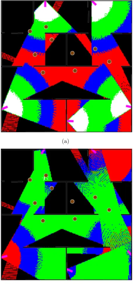
Experiment 3 In the final experiment we apply the algorithm on Map
(a)
(b)
(a)
(b)
provided in Fig. 2.11. Table 2.3 summarizes the results obtained.
Initially there were only five targets in the visible area while all the other targets were not covered. However, after the reconfiguration a total of eight targets have become visible, while only two of them are not visible. The corresponding CT has increased from 0.5461 to 0.8000. Decrease of
the global coverage is in expected range,
From the above experiments it is reasonable to say that performance of the algorithm is consistent across various environment, maintaining in all cases more than 50% improvement in the target coverage.
Table 2.3: Target coverage for Map 3.
Configuration White Green Blue Red Black CT CG
Initial 0 0 1 4 5 0.1973 0.5058
Final 0 4 3 2 1 0.6797 0.4806
2.4.2 3D model evaluation
In this sub section 3D model evaluation is presented, such a model is highly accurate and descriptive. It is very useful when there is no limit on com-putational complexity and requires highly accurate camera configuration.
Scenarios
(a)
(b)
1. Geometry of all walls and floor in terms of planes, in a 3D coordinate system. In case an object cannot be described in geometrical terms, its nearest approximation is obtained as a combination of regular ge-ometric shapes.
2. Texture information of the walls, ground plane, and other objects, described using the POV-ray scene description language.
3. Radiometric properties, as diffusion of light over the surface and re-flectivity.
4. The configuration of the illumination sources has also to be specified (approximately) in terms of color of the light, power, shape, location, and type (circular, cylindrical, parallel, spot etc.)
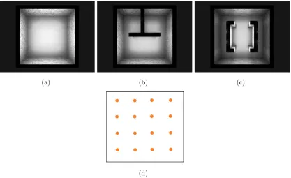
Virtual scenarios In order to test the algorithm, we will report here for the sake of demonstration two different realistic environments of medium size. The first environment (Fig. 2.12(a)) is a large empty hall of 15X15m2 in size, with walls that are 3m high. The room exhibits a texture in light gray. The diffusion of the walls is set to 0.5, and the reflection coefficient to 0.3. The remaining 0.2 corresponds to dissipation.
The second scenario, see Fig. 2.12(b), maintains the same properties of the first map, but in addition we introduce a T-shaped wall in the hall with the center of theT coinciding with origin of the environment reference system. The introduction of the obstacle severely alters the environment in terms of light spread and reflections.
(a) (b) (c)
(d)
Figure 2.12: Overhead view of the three maps and the lighting system.
As far as the lighting system is concerned, 16 white lights, each of them with a wattage of 100W, are uniformly distributed in the environment. We modeled the light source using so-called area lights, consisting of equidis-tant two dimensional array of point light sources whose cumulative wattage is equal to the value specified for the total light source.
Lights are placed at the height of 3m at a distance of 1.4m one from each other both along Z and X (Fig. 2.12(c)). For the attenuation of light we have used an inverse square function.
Real scenario To evaluate the validity of the proposed solution in a real
For a fair comparison we simultaneously record with both systems a video showing people moving arbitrarily in the apartment. After recording we carry out both qualitative and quantitative evaluation. Due to the small size of the evaluation site, coverage is only a limited problem, hence our evaluation mainly focuses on the quality and the information content of the videos. All the details of the space are appropriately modeled, includ-ing color and texture. Even the natural light cominclud-ing from the window is modeled using a small light source. The image of the real scenario and its virtual counterpart are shown in Fig 2.28 and 2.29, respectively.
Evaluation of the camera model
The metrics we have implemented to evaluate the camera positioning, are based on entropy and distortion.
Entropy essentially corresponds to the amount of information, or level of detail measured in the snapshot captured by the camera. It depends on many factors including occlusions, orientation, lighting. However, one element that greatly influences the level of detail in any image is the focal length of the camera. In order to demonstrate the validity of the entropy as a metric, we vary the focal length of the camera from 5mm to 85mm and track the variation of entropy both qualitatively and quantitatively. The environment used for testing (simulated using POV-ray) consists of a large room (sized 4.6×4.85m2, with reflection coefficient 0.3, and a central lighting of 100W) with a sphere of radius 0.5m positioned in the center. The camera is placed image plane points towards the center of the sphere. The origin of the coordinate system is located at the center of the room.
Fig. 2.14. The corresponding focal lengths and entropy values are reported in Table 2.4.
In Figure 2.14(a) most of the details of the environment are visible. Consequently the entropy measure obtained for the image is also high. As the focal length increases, we observe a progressive change in the entropy curve with occasional transients, mainly due to the change in the amount of details present in the captured snapshot. As can be seen from Figure 2.14(b-g) the variation of entropy is heavily dependent on the nature of the environment and the objects being observed. Hence, it is imperative that the camera system continuously re-adapts to optimize itself w.r.t entropy.
0 2 4 6 8 10 12 14 16 18 0.1
0.2 0.3 0.4 0.5 0.6 0.7 0.8 0.9 1
Focal Length
Entropy
Figure 2.13: Variations in the entropy values obtained at different focal lengths.
(a) (b) (c) (d) (e) (f)
Figure 2.14: Images obtained at different focal lengths.
Table 2.4: Entropy and focal length of images Figure Focal Length Entropy Measure
2.14(a) 5 mm 0.9568
2.14(b) 10 mm 0.3697 2.14(c) 25 mm 0.8357
2.14(d) 40 mm 0.5337 2.14(e) 55 mm 0.1274 2.14(f) 85 mm 0.2584
The location of the camera for this particular simulation is the same as in the previous case, the focal Length is set to 4.2mm. The locations of the spheres and mean distortions of each of them are listed in Table 2.5. Spheres are listed in the table following a clockwise arrangement starting from the one closest to the top left corner of the image. Using the camera model and the distortion metric, we have also divided the image into zones of distortion as shown in Figure 2.15. Red areas indicate the maximum distortion, while green areas exhibit the lowest level of distortion. Comparing the two figures 2.15(a,b) and also by looking at the table, we can clearly see that deformity of the spheres increases with the increase in distortion.
Results for virtual test cases
Table 2.5: Distortion and location of spheres Location Distortion
-1,0.25,1.5 0.6400 1,0.25,1.5 0.3828 -1,0.25,.25 0.7018
1,0.25,.25 0.5471 -1,0.25,-.75 0.7511
1,0.25,-.75 0.6560
Figure 2.15: Sample image and distortion zones. Distortion is defined according to Eq. (2.10). Colors corresponds to different levels of distortion: red correspond to µD >0.8, orange 0.8> µD >0.5, yellow 0.5> µD >0.2, and green 0.2> µD >0
one of the cameras (selected randomly) is turned off and the algorithm is again applied to reconfigure in terms of PTZ. The absolute positions of the remaining three cameras remain the same, as they are already deployed (installed). Similarly to the previous scenario, another camera is turned off and the reconfiguration is performed for the remaining cameras in order to readjust the setup.
The radiometric constants used for the virtual environment are tabu-lated in Table 2.6.
Table 2.6: Environment radiometric constants Property Constant
Fade distance 0.2
Fade power 2 Diffusion 0.3 Turbulence 1
multiple cameras, unless specifically requested), while maximizing the qual-ity of the captured data. Placement locations along the walls have been quantized at the rate of 0.5m both in X and Z. The focal length range has been varied from 5mm to 85mm in steps of 5mm, while pan and tilt
vary from 0◦ to 180◦ and 0◦ to 90◦, respectively at steps of 1◦.
Figure 2.17 shows the snapshots obtained from the cameras after the initial positioning. The total coverage obtained is 76.43%. As can be seen from Table 2.7, whenever the coverage of the individual camera is very small, it is compensated by low levels of distortion and high entropy, since our formulation assigns equal importance to both coverage and quality.
The final coverage map is shown in Figure 2.16(a). For the sake of visualization, a color code is used to describe the density of the rays that intersect the cells of the grids. Cells colored in white, correspond to more than 100 rays per cell, whereas green represents areas, which ray density is between 10 and 100. Blue regions have a ray density between 1 and 10, and red areas have only one ray per cell. We can also observe from the results that the area of intersection between FOVs of the individual cameras is limited, which is one of the objectives of optimization.
Table 2.7: Map1: Entropy and distortion after the initial setup. Cam ID Entropy µD σ2D Coverage (%)
1 0.2085 0.5566 0.2278 15.18 2 0.8935 0.4832 0.1952 3.07
(a) (b) (c)
Figure 2.16: Map1: total coverage map after initial placement (a), reconfiguration 1 (b), and 2 (c).
After the initial positioning, we now turn off the fourth camera, simu-lating a malfunctioning. Due to the malfunction the system setup becomes sub-optimal. In order to improve its performance, reconfiguration has to be performed in terms of pan, tilt, and zoom, as the absolute positions are fixed. The algorithm is then applied again, and the configuration is up-dated. The resulting snapshots from the cameras are shown in Figure 2.18. Table 2.8 lists the individual distortion and entropy metrics of the cameras. The area covered reduces to 61%, compared to the 54%, which would have been the case, if reconfiguration was not run. The overall coverage map is provided in Figure 2.16(b). As can be seen from Table 2.8, camera 2 has extended the coverage area in order to compensate for the loss of one camera in the network. Subsequently, its covered area has doubled, while the entropy has halved.
Table 2.8: Map1: entropy and distortion after reconfiguration 1 Cam ID Entropy µD σ2D Coverage (%)
1 0.2124 0.5474 0.2139 14.87
2 0.4912 0.6216 0.3620 6.92 3 0.1479 0.4393 0.0661 40.13
4 OFF OFF OFF OFF
Figure 2.18: Map1: snapshots from the three cameras after reconfiguration 1.
Figure 2.16(c), while Table 2.9 showcases the quality metrics of the indi-vidual cameras. The overall coverage has reduced to about 45%, compared to 21.22%, the coverage obtained with only two cameras before reconfigu-ration.
Table 2.9: Map1: entropy and distortion after reconfiguration 2. Cam ID Entropy µD σ2D Coverage (%)
1 0.2124 0.5474 0.2139 14.87 2 0.4912 0.6216 0.3620 40.42
3 OFF OFF OFF OFF
4 OFF OFF OFF OFF
Figure 2.19: Map1: snapshots from two cameras after reconfiguration 2.
Evaluation for Map2 In this case Map 2 is subjected to the same se