Indoor Positioning Method Based on Wireless Signal

Indoor Positioning Method Based on Wireless Signal

Jingjing Yang, Zhenyu Feng, Xuchao Ma, Xiao Zhang(*₎

Hebei North University, Zhangjiakou, China [email protected]

Abstract—In view of the problems of traditional wireless indoor positioning technologies such as errors and a low positioning accuracy that cannot reach the application level required by hospital indoor positioning, this study proposes a hospital indoor positioning method based on wireless signals. This study firstly analyzes the principles of hospital indoor positioning, verifies the reliability and accuracy of the collected data using Gaussian distribution, P-P plot and Q-Q plot, and finally analyzes the collected data using the least square fitting algorithm to obtain a fitting wave attenuation model, which is then applied to the indoor posi-tioning system. Experiments show that this method can reduce the error of indoor positioning in hospitals, and improve the repeatability and measurement accuracy of indoor positioning in hospitals.

Keywords—Indoor positioning, Wireless signal, Gaussian distribution, Fitting wave attenuation model

1

Introduction

The application of various positioning technologies in hospitals has been at the ex-perimental and trial level, and they have gradually been adopted until in recent years. However, because various positioning has its own advantages and disadvantages, only by selecting the appropriate cost-effective solutions and integrating applications with each other, can we obtain more effective precise positioning points and improve prac-ticality.

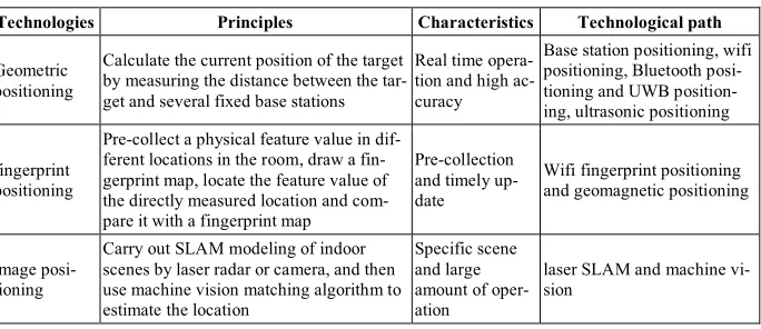
Table 1. Comparison of indoor positioning principles

Technologies Principles Characteristics Technological path

Geometric positioning

Calculate the current position of the target by measuring the distance between the tar-get and several fixed base stations

Real time opera-tion and high ac-curacy

Base station positioning, wifi positioning, Bluetooth posi-tioning and UWB position-ing, ultrasonic positioning

fingerprint positioning

Pre-collect a physical feature value in dif-ferent locations in the room, draw a fin-gerprint map, locate the feature value of the directly measured location and com-pare it with a fingerprint map

Pre-collection and timely up-date

Wifi fingerprint positioning and geomagnetic positioning

image posi-tioning

Carry out SLAM modeling of indoor scenes by laser radar or camera, and then use machine vision matching algorithm to estimate the location

Specific scene and large amount of oper-ation

laser SLAM and machine vi-sion

Due to the popularization and low development costs of wireless hotspots, poor ac-curacy and high volatility of conventional wireless signal base stations, Gaussian fitting and least square fitting algorithm are used to analyze the collected data to obtain the fitting wave attenuation model as the principle of hospital indoor positioning, which can reduce costs, and improve repeatability and measurement accuracy.

2

The styles

According to the relationship between signal intensity and distance, the traditional wave propagation model is studied [9]. In an ideal space environment, wall blocking and multipath propagation effects are not considered. Assuming that the distance be-tween the wireless signal transmitting end and the wireless signal receiving end is d, the receiving power of the receiving end may be denoted as [10]:

𝑃𝑃"(𝑑𝑑) ='()()*+

,

(-.),_/,₀ (1)

In the formula (1), P2is the transmitter transmit power, G4 and G5 are the power am-plifications of transmitting and receiving antenna respectively, λ represents the wireless wave wavelength, the unit of P2 and P2 is W, and G4 and G4are dimensionless. From the above formula, it can be obtained that the distance d7 _{is inversely proportional to the} receiving power under ideal conditions.

In real environment, there are multi-path propagation, obstacle reflection, signal dif-fraction and so on, so the ideal wireless propagation loss model is not applicable. There-fore, the logarithmic-normal distribution model is adopted Fehler! Verweisquelle konnte nicht gefunden werden.:

𝑃𝑃8(𝑑𝑑) = 𝑅𝑅𝑅𝑅𝑅𝑅𝑅𝑅 = 10 lg @'A(/_'B)C + 20lg [/_/B] (2)

requirements, the wireless signal attenuation model based on the RSSI ranging algo-rithm is simplified Fehler! Verweisquelle konnte nicht gefunden werden. as:

RSSI=A-10nlgd (3) Where, in the formula (3),d is the distance between the wireless base station and the user, whose unit is m. A is the RSSI measured when the distance d between the wireless base station and the user is equal to 1 m, and n is the signal attenuation factor. As dif-ferent materials have difdif-ferent signal absorption rates, n has difdif-ferent values. Consider-ing the absorption of signals by housConsider-ing materials, n ranges from 3 to 4.

Since, conventional wave propagation attenuation model has many shortcomings [8], data is collected according to the traditional wave model. According to the principle of statistics, the wave propagation attenuation model is fitted by the least square fitting polynomial based on the traditional model, so as to make it more conform to the actual model.

Under normal circumstances, the calculated received signal strength always has an error from the actual situation, because the field strength is inversely proportional to the distance and the complex terrain of the actual environment leads to weakening sig-nals [11]. In addition to the cause of equipment failure, the distance d from the wireless base station to the user location obtained by the signal attenuation model is generally greater than the real distance. As shown by the left figure in Figure 1, the distances between every two points of user location D and the wireless base stations A, B, and C are calculated respectively based on the RSSI model. A circle is made using the sites and calculated distance, then the intersection point can be obtained.

The basic idea of the centroid positioning algorithm [12] is as follows: Calculate the intersection points of three circles, in which each two are intersecting, then six inter-section points are obtained, wherein the three points closest to the user are feature points, which are represented by E, F and G. The feature point is taken as the vertex of the triangle, the centroid of the triangle as the predicted point M where the user is lo-cated. The feature points E, F and G are as shown in Figure 1. The calculation method of the feature point E is:

(4) Similarly, the coordinates of F and G can be calculated. At this time, the coordinates of the unknown point are

@

O

,

QKLQMLQN O

C

In Figure 1, D represents the actual location of the user, and M represents the user's location calculated by the centroid algorithm. Then the algorithm is compared with an-other positioning algorithm, trilateration method, through which the user’s coordinate point is estimated to be N. Through the comparison with the two methods, it can be known that the accuracy of the centroid algorithm is higher.

x_e−x_a

(

)

+

(

)

(

)

+

(

)

=rb

x_e−x_c

(

)

+

(

)

Fig. 1. Trilateration and centroid positioning

3

Fitting Process of Wave Propagation Attenuation Model

3.1 Data acquisition

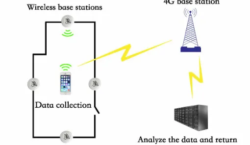
The data acquisition part of this design mainly consists of wireless signal base sta-tion, mobile phone based on iOS operating system, mac computer based on 10.13 op-erating system and SQL database. The overall data acquisition structure is shown in Figure 2.

During the measurement, the signal base stations are arranged in a symmetrical man-ner. In this design, 10 base stations are arranged in a circular manman-ner. The signal acqui-sition end is in the center of the ring, thus the vertical field intensity vector is cancelled. Set the abscissa of the distance, and the coordinates are from 0.05 to 2.1. 0.05 is the step size of 0.05-0.1, 0.1 is the step size of 0.1-1, and 0.2 is the step size of 0.1-2.1. There are a total of 17 coordinate points as follows: [0.05,0.1,0.2,0.3,0.4,0.5,0.6,0.7,0.8,0.9,1,1.2,1.4,1.6,1.8,2,2.1].

Set the acquisition time interval to 1s, and each RSSI intensity value is collected. When the number is greater than 500 signal points, the distance is moved according to the above table. Data exported from the SQL database is saved as a data file of dat.csv and the actual number of collected data is 89,328.

3.2 Data exploration

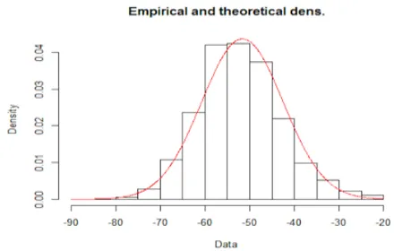
Data exploration [13] verifies the reliability and accuracy of this set of data in terms of Gaussian distribution, P-P plots, and Q-Q plots. Gaussian distribution is used to in-tuitively judge whether Gaussian distribution is met or not, and P-P plots and Q-Q plots are used to verify the correctness of intuition.

Since there are many non-negligible influencing factors in the indoor propagation process of signals, such as multipath propagation effect, background noise, reflection, etc., the relationship between RSSI and the distance D is not a one-to-one correspond-ence in actual situations, but a one-to-many relationship. It can be seen from the above that the RSSI may dither. Therefore, the reliability of the data can be judged by deter-mining whether the data conforms to the normal distribution. It can be seen from Figure 3 that the data distribution conforms to the Gaussian distribution model.

The P-P plot reflects the relationship between the cumulative ratio of the specified distribution and the cumulative ratio according to the variable. P-P plot can show whether the data conforms to the specified distribution. When all the points in the P-P plot approximately is in a straight line, it indicates that the data conforms to the speci-fied distribution, otherwise it does not. The data of dat.csv is used here.

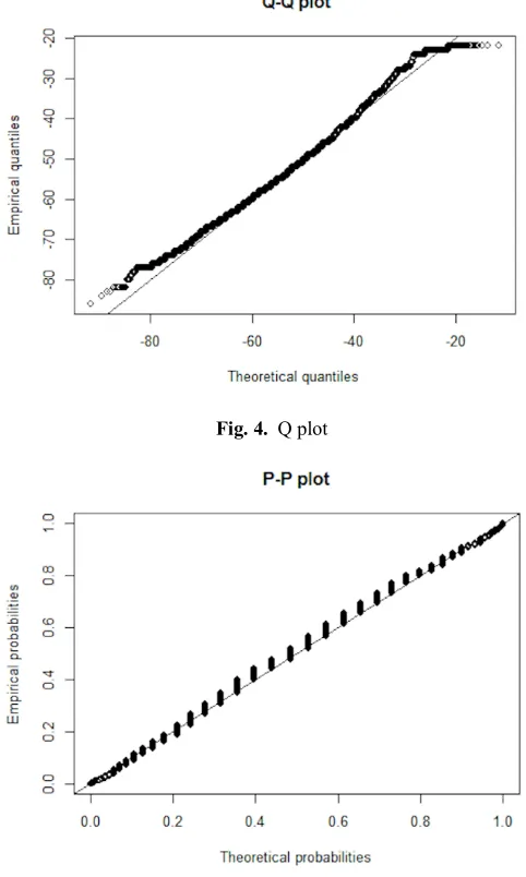
In statistics, the Q-Q gplot (Q represents the quantile) is a probability plot that com-pares the two probability distributions graphically to see if they are similar. If the two distributions have linear correlations, most of their points on the Q-Q plot will fall on a straight line. If the studied distributions are in the position-scale category, the parame-ters can be visually evaluated using a Q-Q plot. First, select the quantile interval, the theoretical quantile interval is -20, and the empirical quantile interval is -10. The dat.csv data is used here.

It can be judged whether the collected sample data conforms to the normal distribu-tion by checking whether the points on the Q-Q plot fall on a straight line or approxi-mately a straight line. Moreover, the slope of the line reflects the standard deviation, and the intercept is the mean value of the sample. As can be seen from the figure, a small amount of data is slightly shifted at both ends, and a large amount of data in the middle corresponds to a Gaussian distribution. The purpose of Q-Q plot is the same as that of P-P plot, whose difference lies in test methods.

The Q-Q plot and the P-P plot verify the normality of the data, such as the Q-Q plot shown in Figure 4 and the P-P plot shown in Figure 5.

Fig. 4. Q plot

3.3 Data exploration

Since the collected data is discrete, the data is described before data fitting using Box-plot, which is commonly used in statistics.

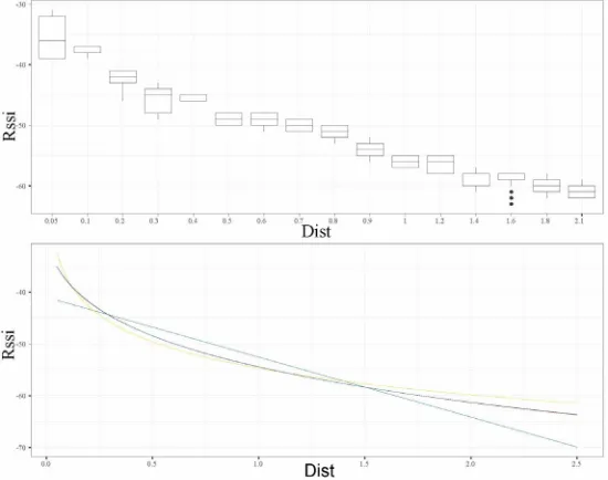
The preprocessed data is used to draw the Box plot, as shown in Figure 6, where the range, median, and outliers of the preprocessed data can be seen.

Data processing is performed according to the pre-data box-plot. The data in the range of [0.3, 0.7] of each group are retained as shown in Figure 7, and the outliers are removed from the processed data, so that the correspondence of that the data reflect is more clear.

Fig. 6. Box-plot of preprocessed data

The Box-plot reflects the correspondence between D (Dist) and Rssi to a certain extent.

The result derived from Formula (1) is a theoretical model, which has certain differ-ences from reality. The Box-plot intuitively reflects an approximately linear relation-ship. However, a logarithmic relationship between Rssi and lgD can be obtained from the theoretical model. So polynomial fitting of lgD and Rssi is carried out. As shown in Figure 8, the green line is a linear fitting of Rssi and D, the yellow line is a linear fitting of Rssi and lgD, the blue line and the red line are the high order fittings of Rssi and lgD. The specific Formulas and their corresponding fitting analysis plots, including Figure 9-1, 9-2, 9-3, and 9-4 are as follows.

(5)

The Residuals section provides the main statistics of the prediction error.

The Coefficients section provides the specific values for each parameter and the pre-dictability of each feature. Three stars indicates that this feature cannot be a variable that has nothing to do with the dependent variable, that is, the relationship between the feature and the dependent variable is extremely strong. Estimate is the estimation of the parameter, Std.Error is the standard deviation of the regression parameter sd (parame-ters), and t value and Pr (>|t|) are all test hypotheses for the regression parameter. t is the t-value of the test hypothesis for the parameter. Pr is used to compare with the sig-nificance level to decide whether to accept the hypothesis test.

Fig. 8. Fitting line

The multivariate R-squared (decision coefficient R-squared) provides a measure of model performance Fehler! Verweisquelle konnte nicht gefunden werden., showing that the model interprets the credibility of the change in the dependent variable value from the overall data. The higher the reliability that the fitted model interprets data, the closer the multivariate squared value is to 1.0. For example, the multivariate R-squared value of the func-3 function is 0.9468, so 95% of the variation rules of the dependent variable can be explained by the model.

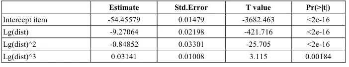
Table 2 summarizes the formula residuals in the above figure. Table 3, Table 4, Ta-ble 5, and TaTa-ble 6 summarize the coefficients of the formulas (5).

Table 2. Residual range of each formula

Min 1Q Median 2Q Max

5-1 -4.5955 -2.0660 -0.5364 1.4636 10.5715

5-2 -6.4659 -1.0783 0.1791 1.5723 3.0621

5-3 -4.385 -1.339 0.234 1.216 4.097

5-4 -4.4210 -1.3300 0.2586 1.1917 4.1427

Table 3. The parameters of Formula 5-1

Estimate Std.Error T value Pr(>|t|)

Intercept item -40.9931 0.0332 -1234.9 <2e-16

Dist -11.5682 0.0304 -380.6 <2e-16

Table 4. The parameters of Formula 5-2

Estimate Std.Error T value Pr(>|t|)

Intercept item -54.70131 0.01333 -4102.6 <2e-16

Lg(dist) -7.39960 0.01256 -589.2 <2e-16

Table 5. The parameters of Formula 5-3

Estimate Std.Error T value Pr(>|t|)

Intercept item -54.427228 0.011604 -4690.5 <2e-16 Lg(dist) -9.290632 0.021029 -441.8 <2e-16 Lg(dist)^2 -0.947378 0.009085 -104.3 <2e-16

Table 6. The parameters of Formula 5-4

Estimate Std.Error T value Pr(>|t|)

Intercept item -54.45579 0.01479 -3682.463 <2e-16 Lg(dist) -9.27064 0.02198 -421.716 <2e-16 Lg(dist)^2 -0.84852 0.03301 -25.705 <2e-16

4

Experiment and Verification

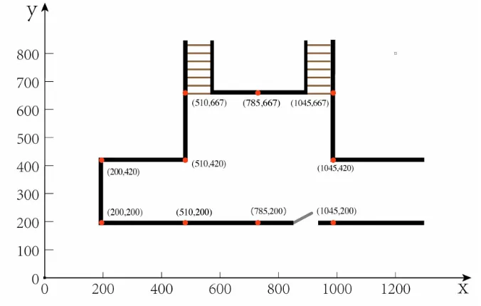
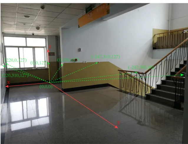
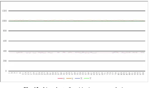
The indoor positioning performance of this design is tested in detail. The macOS High Sierra version 10.13.4 is used on the PC side and the iOS version 11.2.5 is used on the terminal iPhone. In this study, a set of experimental data are analyzed, the results of trilateration centroid positioning algorithm and verification observation algorithm implemented by C code are compared with the actual results, and the errors of the two algorithms are compared. The plan of the experimental site is as shown in Figure 10. The red dot indicates the location of the base station, and the real pictures of the exper-imental site are shown in Figures 11 and 12, and the space coordinate system is drawn by the red line. The green dotted line represents the space vector for each wireless base station. At (368, 990, 127), data is collected per second for a period of 100 s. Table 7 shows the results of calculation variance and mean square error of partial experimental data and all data.

Fig. 11. Real picture of the experimental site

Table 7. Partial data and error analysis

The error data is analyzed. The calculated user coordinate points (x, y) and the user's actual coordinate points (X, Y) are drawn. It can be clearly seen from the Figures 13 that there is not great difference between the calculated user’s coordinate points and the actual coordinate points.

Fig. 13. Line chart of positioning error analysis

Conclusions: Through the comparison of the error and variance of the data, it can be seen that the error fluctuation is better than the range of 0.5m~1m obtained in the past researches, as the error range of this system is 0.2~0.7.

5

Conclusions

As the hospital has strengthened its efforts in informatization and intelligent con-struction in recent years, the indoor positioning technology studied in this paper will play a more active role in the medical care of the hospital.

(x,y) (X,Y) Error(cm) Vari-_ance square devi-Mean ation

(x, y) as a theoretical coordinate point

(X, Y) for calculating coordinates

The lower right cor-ner of a plane map is the origin of the

coor-dinates

(368,990) (364.09762,1017.0585) 27.33

16.38 4.028 (368,990) (366.79742,1015.2148) 25.24

6

Acknowledgment

This project was supported partially by Population Health Informatization in Hebei Province Engineering Technology Research Center, Medical Informatics in Hebei Uni-versities Application Technology Research and Development Center and Zhangjiakou Municipal Science and technology and Seismological Bureau (No.1711038C).

7

References

[1]He, S., Chan, S.H.G. (2016). Wi-Fi fingerprint-based indoor positioning: Recent ad-vances and comparisons. IEEE Communications Surveys & Tutorials, 18(1): 466-490. DOI: 10.1109/COMST.2015.2464084 https://doi.org/10.1109/COMST.2015.2464084

[2]Cannistraro, M., Bernardo, E. (2017). Monitoring of the indoor microclimate in hospi-tal environments a case study the Papardo hospital in Messina. International Journal of Heat and Technology, 35(1), S456-S465.. https://doi.org/10.18280/ijht.35Sp0162

[3]Liuzzi, S., Stefanizzi, P. (2016). Experimental study on hygrothermal performances of in-door covering materials. International Journal of Heat and Technology, 34(2), S365-S370. DOI: 10.18280/ijht.34Sp0225. https://doi.org/10.18280/ijht.34Sp0225

[4]Kanaan, M., Chahine, K. (2018). CFD study of ventilation for indoor multi-zone transformer substation. International Journal of Heat and Technology, 36(1), 88-94. DOI: 10.18280/ijht.360112. https://doi.org/10.18280/ijht.360112

[5]Yang, C., Shao, H.R. (2015). WiFi-based indoor positioning. IEEE Communications Mag-azine, 53(3): 150-157. https://doi.org/10.1109/MCOM.2015.7060497

[6]Hossain, A.K.M.M., Soh, W.S. (2015). A survey of calibration-free indoor positioning sys-tems. Computer Communications, 66: 1-13. https://doi.org/10.1016/j.comcom.2015.03.001

[7]Yang, H., Yang, S. (2010). Connectionless Indoor Inventory Tracking in Zig Bee RFID Sensor Network. 2009 25th annual conference of IEEE industrial electronic, 1-6: 2470-2475. [8]Yang, J., Wang, Z., Zhang X. (2015). An ibeacon-based indoor positioning systems for

hos-pitals. International Journal of Smart Home, 9(7): 161-168. https://doi.org/10.14257/ijsh.20 15.9.7.16

[9]Elson, J., Girod, L., Estrin, D. (2002). Fine-grained network time synchronization us-ing reference broadcasts. ACM SIGOPS Operating Systems Review, 36(SI): 147-163. [10]Liu. C., Wu, K., He, T. (2005). Sensor localization with ring overlapping based on

compar-ison of received signal strength indicator. Mobile Ad-hoc and Sensor Systems IEEE Inter-national Conference on, 2(56): 516-518. https://doi.org/10.1109/MAHSS.2004.1392193

[11]Al-Madani B.M., Shahra E.Q. (2018). An Energy Aware Plateform for IoT Indoor Tracking Based on RTPS. Procedia computer science, 130(C): 188-195. https://doi.org/10.1016/j.pro cs.2018.04.029

[12]Casetti E., Can A. (1986). Trigonometric expansions: An application to the study of migra-tion fields. Modeling and Simulamigra-tion, 17(1): 23-28.

8

Authors

Jingjing Yang received his Master Degree from Lanzhou Jiaotong University in 2012. Now he is a doctoral student at the University of Chinese Academy of Sciences and he is currently a lecturer of the school of information science and engineering at Hebei North University. His research interests are in the field of image processing and internet of things.

Zhenyu Feng is the member of Population Health Informatization in Hebei Province Engineering Technology Research Center. His research interests are in the field of in-ternet of things.

Xuchao Ma is the member of Population Health Informatization in Hebei Province Engineering Technology Research Center and Medical Informatics in Hebei Universi-ties Application Technology Research and Development Center. His research interests are in the field of internet of things.

Xiao Zhang is a Professor of the school of information science and engineering, Hebei North University, Zhangjiekou, China. He has published in various National, International Journals and Conference papers. He has 30 years of Teaching Experience. His areas of interests are media security and signal processing.