Published online August 20, 2014 (http://www.sciencepublishinggroup.com/j/acm) doi: 10.11648/j.acm.20140304.17
ISSN: 2328-5605 (Print); ISSN: 2328-5613 (Online)
Regularized minimum length method in scattered data
interpolation
Guang Y. Sheu
Department of Accounting and Information Systems, Chang-Jung Christian University, Tainan, Taiwan
Email address:
[email protected]To cite this article:
Guang Y. Sheu. Regularized Minimum Length Method in Scattered Data Interpolation. Applied and Computational Mathematics.
Vol. 3, No. 4, 2014, pp. 163-170. doi: 10.11648/j.acm.20140304.17
Abstract:
In an attempt of accumulating more experiences of interpolating scattered data using the minimum length method, this study chooses new kernel functions from the machine learning technique to implementing this minimum length method. But, consulting with the regularization theory, a regularized minimum length method is created by solving coefficient of it in a penalized least squares approximation problem. The purpose of creating this regularized minimum length method is responding to a pilot observation finding the instability of original minimum length method under dense interpolation points. Testing the regularized minimum length method finds that applying it is time-saving but its performance is comparable to the radial point interpolation with polynomial reproduction. Inverse multiquadric and rational quadric kernel functions are two preferred kernel function to perform the regularized minimum length method. In conclusion, the proposed regularized minimum length method can be a useful scattered data interpolation method.Keywords:
Regularized Minimum Length Method, Machine Learning, Scattered Data Interpolation1. Introduction
Many methods such as the radial point interpolation with polynomial reproduction [1] and moving least squares approximation are available for interpolating a function over scattered points. But, it is still interested in searching more time-saving alternatives but still obtaining sufficiently accurate interpolation results. The minimum length method [2] may be an example of such alternatives. Originally, it is a computational technique for solving underdetermined inverse problems. For example, Liu, et al. [3] applied this minimum length method to construct geostatistical reduced-order model. Kamm [4] applied the minimum length method to the inversion of electromagnetic and potential field data. But, the minimum length method had been used to scattered data interpolation [5]. In this literature [5], an interpolation formula is derived by minimizing the squared sum of its coefficients. In addition, solving these coefficients inverts some matrices once. Since inverting some matrices twice is required in implementing the radial point method with polynomial reproduction, the minimum length method is consequently computationally cheaper. Unfortunately, no further studies were devoted to evaluate the minimum length method in scattered data
interpolation; therefore, experiences of such as available choices of kernel functions and the stability of minimum length method were not discussed.
In order to accumulate more experiences of using the minimum length method as a scattered data interpolation method, this study implements it using new kernel function, which come from the machine learning technique [6-8]. In addition, responding to a pilot observation finding the instability of original minimum length method under dense interpolation points, a regularized minimum length method is created by solving coefficients of it through a penalized least squares approximation problem [9]. Preferred kernel functions and how to set required parameters for applying the regularized minimum length method are then searched through two interpolation experiments.
2. Regularized Minimum Length
Method
Suppose x and y are spatial coordinates and a function u(x, y) to be interpolated using M scattered interpolation points (x1, y1), (x2, y2)… (xM, yM). To estimate u(x, y) at an
interested point (xQ, yQ), a local support domain ΩQ is
within this ΩQ, this study approximates u(x, y) over the ΩQ
by
1 1
T T
( , ) ( , ) ( , )
B a P b
N m
i i j j
i j
u x y B x y a p x y b
= =
≈ +
= +
∑
∑
(1)
where ai (i = 1, 2,…N) and bj (j = 1, 2,…m) are coefficients
to determined, Bi(x, y) (i = 1, 2,…, N) is called as the
kernel function in this study, p1(x, y), p2(x, y),…, pm(x, y)
denote a complete monomial basis of m terms, BT = [B1(x,
y), B2(x, y),…, BN(x, y)], a = [a1, a2,…, aN]T, b = [b1,
b2…bm]T, and PT = [1, x, y,…, pm(x,y)]. To solve unknown
coefficients in (1), this equation is computed at each interpolation point within the ΩQ. Accounting for the
possible interpolation errors, interpolation results are expressed by
δδδδ + + =B a Pb
U 0 0 (2)
where U = [u(x1,y1), u(x2,y2),…, u(xM, yM)]T, (x1,y1),
(x2,y2),…, (xN, yN) denote those interpolation points within
the ΩQ of point (xQ,yQ), δ = [δ1, δ2,…, δN]T, δi (i = 1, 2…N)
is the interpolation error at the point (xi, yi) and
1 1 1 2 1 1 N 1 1
1 2 2 2 2 2 N 2 2
0
1 N 2 N N N
B ( , ) B ( , ) B ( , )
B ( , ) B ( , ) B ( , )
B
B ( , N) B ( , N) B ( , N)
x y x y x y
x y x y x y
x y x y x y
= ⋯ ⋯ ⋮ ⋮ ⋱ ⋮ ⋯ (3)
1 1 1 1
2 2 2 2
0
N N
1 x ( , )
1 x y ( , )
P
1 x y ( , )
m
m
m N N
y p x y p x y
p x y
= ⋯ ⋯ ⋮ ⋮ ⋯ ⋱ ⋮ ⋯ (4)
Nevertheless, (2) is underdetermined, since this equation contains (2N + m) unknowns ai (i = 1, 2…N), bj (j = 1,
2….m), and δi but only N equations are available for
solving these unknowns. To uniquely solve ai, bj, and δi, a
penalized least squares approximation problem is defined: Consulting with the regularization theory (see, e.g. [10-11]), the goal is finding those ai, bj, and δi, values to mimimize
the following Lagrangian functional Π:
Π= + + λ U − B a − P b − δ (5)
where γ is an error parameter for controlling interpolation errors, λT = [λ
1, λ2…λN], and λi is the Lagrangian multiplier.
In (5), the term (aTa + bTb)/2 controls the smoothing of (1);
whereas, the final term λT(U - B0a - P0b - δ) imposes
constraints. Meanwhile, γδTδ/2 denotes a regularization term.
(see, e.g. [10-11]) It measures the closeness to the data of u(x, y). If a large γ is adopted, increased the pointwise accuracy is expected. The other reason why the regularization term γδTδ/2 is added is responding to a pilot observation finding
the instability of original minimum length method under dense interpolation points. At such a situation, the
collocation matrix B0 is ill-conditioned, since one row of the
matrix of B0 differ slightly from the other row.
The adoption of regularization terms was also seen in applying such as the least squares support vector machine technique [12], neutral networks [13], and Bayesian methods [14]. The uses of regularization terms include the
improvement of overprediction phenomenon [12],
performance of neutral networks [13], and stability of interpolation results [14].
Next, computing the derivatives of Π with respect to unknowns a, b, e, and λ yields
λλλλ
T 0
0 a B
a = ⇒ =
∂ Π ∂ (6a) λλλλ T 0
0 b P
b = ⇒ =
∂ Π ∂
(6b)
δδδδ
λλλλ = ⇒ = + +
∂ Π ∂ b P a B
U 0 0
0 (6c)
λλλλ δδδδ δδδδ = ⇒γ = ∂
Π ∂
0 (6d)
Substituting (6a), (6b), and (6d) into (6c), we can obtain
λ as follow:
U I P P B B 1 T 0 0 T 0 0 − γ + + =
λλλλ (7)
where I is an identity matrix. In (7), a term I/γ exists due to the adding of term γδTδ/2 in (5). Since (7) contains the term
I/γ, we can ensure that matrix λ is invertible. Meanwhile, substituting (7) into (6a), (6b), and (6d) results in
-1
T T T
0 0 0 0 0
I
a = B B B + P P + U
γ
(8a)
-1
T T T
0 0 0 0 0
I b=P B B +P P + U
γ
(8b)
1
T T
0 0 0 0
1 I
B B P P U
−
δ = + +
γ γ (8c)
Further substituting (8a)… (8c) into (1) yields
1
T T T T T T
0 0 0 0 0 0
I
u(x, y) (B B P P ) B B P P U
−
≈ + + +
γ
(9)
Since inverting some matrices once is required in computing (9), this equation is still computationally cheaper than the radial point interpolation method with polynomial reproduction [1]. Moreover, derivatives of (9) is computed by
T T T T
0 0
1
(B )B (P )P T T
0 0 0 0
x x
u
I
B B
P P
U
x
− ∂ ∂ ∂ ∂
∂
≈
+
+
+
T T T T
0 0
1 (B )B (P )P T T
0 0 0 0
y y
u I
B B P P U
y − ∂ ∂ ∂ ∂ ∂ ≈ + + +
∂ γ (10b)
3. Interpolation Experiment I
Consider an interpolation experiment [15] in which the following function is to be interpolated:
] 10 , 0 [ ] 10 , 0 [ ) y , x ( 5 . 1 ) cos( ) ( sin ) y , x (
u 210x 210y
× ∈
+
= π π
(11)
The main goal of interpolating (11) and its derivative is preliminarily searching preferred kernel functions to compute (9), (10a), and (10b). Using these preferred kernel functions, it is desired that the performance of these equations is comparable to the radial point interpolation method with polynomial reproduction (See Ref. [15] for the details of. this radial point interpolation method with polynomial reproduction).
Unless otherwise stated, follow the next seven steps to determine the required data in interpolating (11) and its derivatives:
(1) Approximate u(x, y) and its derivatives at 100 interested points. Coordinates of these points are (x, y) = [0.4 + (i-1), 0.4 + (j-1)] (i, j = 1, 2…10). At each interested point, choose a circle local support domain Ω centered at this point. Set the radius ρ of each Ω equal to 3.5.
(2) Create 6×6 (M = 36) to 21×21 (M = 441) equally spaced interpolation points over the region (x, y) ∈ [0, 10] × [0, 10]. In other words, if h is the spacing of any two connecting interpolation points, it will be between 2.0 and 0.5.
(3) Adopt a complete monomial basis of one term; i.e. m = 1 or PT = [1].
(4) Choose five kernel functions from the machine learning technique [6-8] to be Bi(x, y) (i = 1, 2…N).
Table 1 lists these 5 kernel functions in which σ, q, and c are shape parameters and r is the Euclidean distance between two points.
Table 1. Kernel functions for the current study
Name Expression Shape
parameters
Rational quadric σ/(r2 + σ) σ
Spherical 1-3r/2σ+0.5(r/σ)3 σ
Inverse multiquadric (r2+σ2)-q σ, q
Circular 2cos-1(-r/σ)/π-2r(1-(r/σ)2)1/2/(πσ) σ
Generalized T-student 1/(1+rc) c
(5) Set γ = 0 in searching the proper values of shape parameters σ, q, and c. Investigate subsequently variation of interpolation errors with respect to nonzero γ values; therefore, the proper γ value can be determined.
(6) Perform the radial point interpolation method with polynomial reproduction using the multiquadric
radial basis function, R = [r2 + (αcdc)2]q in which αc and q are shape functions, and dc is the
characteristic length or averaged nodal spacing. Set
αc = 1.0, q = 1.03, and dc = 3.5 [11].
(7) Quantify the accuracy of interpolation results using the following averaged interpolation errors ξ, ζ, and
ε:
∑
= − = ξ 100 1 i i exact num exact u u u 100 1 (12a)∑
= ∂ ∂ ∂ ∂ ∂ ∂ − = ζ 100 1 i i x u x u x u exact num exact 100 1 (12b)∑
= ∂ ∂ ∂ ∂ ∂ ∂ − = ε 100 1 i i y u y u y u exact num exact 100 1 (12c)where the superscript exact notes the exact results, the superscript num notes the numerical results, and the subscript i denotes the i-th interested point.
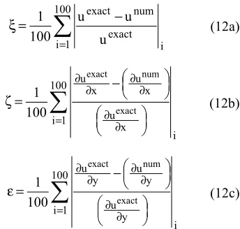
3.1. Searching Preferred Kernel Functions
Adopt M = 121, γ = 0, and ρ = 3.5 or 2.5. Figs. 1(a)...1(f) show variation of averaged interpolation ξ with respect to different types of kernel functions and their shape parameters. In plotting these six figures, the range of shape parameters is determined by inspecting corresponding interpolation errors. This inspection continues until obtaining less interpolation errors is impossible.
Among five kernel functions in Table 1, Figs. 1(a)…1(f) indicate that the inverse multiquadric, rational quadric, and circular kernel functions may be three preferred kernel functions. If these three types of kernel functions are used, obtaining less interpolation errors is expected. For example, if we use ρ = 3.5, σ = 40, and the rational quadric kernel function to compute (9), Fig. 1(a) indicates that the interpolation error ξ is less than 0.02.
In addition, Figs. 1(a)…1(f) demonstrate that decreasing the radius ρ may give more proper values of shape parameters. For example, if we use the spherical kernel function to compute (9), changing the ρ value from 3.5 to 2.5 permits the use of σ = 1.0 without obtaining unsatisfactory ξ values. Consequently, ξ(ρ = 2.5 and σ = 1.0) ≈ 0.025 and ξ(ρ = 2.5 and σ = 1.0) ≈ 0.09 are obtained in plotting Fig. 1(b).The latter ξ value is unsatisfactory.
3.2. Comparison of Interpolation Results
obtained using the rational quadric, circular, and inverse multiquadric kernel functions, these three types of kernel
functions are used in this section.
Figure 1.Search of preferred kernel functions to compute (9), (10a), and (10b) (M = 121, γ = 0)
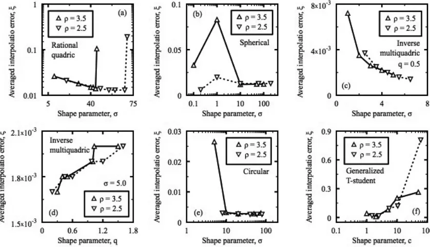
Set γ = 0 and select values of shape parameters from Figs. 1(a), 1(c), 1(d), and 1(e). Figs. 2(a)…2(c) compare variation of interpolation errors ξ with respect to different h values and kernel functions in which RPIM denotes the radial point interpolation method with polynomial reproduction. The chosen values of shape parameters are listed inside these figures.
Observing Figs. 2(a)…2(b) can easily find the interpolation errors ξ approach uncontrollably in the range 0.5 ≤ h < 1. These two figures confirm the aforementioned pilot observation finding the instability of original minimum length method under dense interpolation points. In an attempt of improving these uncontrollable interpolation errors, three methods are found:
(1) Adopt multiple ρ values. For example, we can use ρ = 2.5 in the range 0.5 ≤ h < 1 and ρ = 3.5 for other h values.
(2) Use special kernel function to be Bi(x, y) (i = 1,
2…N). Fig. 2(c) is an example. Even if γ = 0 is set, this figure demonstrates that the circular kernel function doesn’t cause the instability of (9) in the range 0.5 ≤ h < 1. Consequently, interpolation errors
ξ approach limitedly in Fig. 2(c). However, it should be simultaneously noted that (9) interpolates u(x, y) less accurately when the circular kernel function serves as Bi(x, y).
(3) Use nonzero γ values. Figs. 3(a)…3(b) illustrate two example. Creating these two figures modifies Figs. 2(a)…2(b) with setting γ = 1012. Observing Figs. 3(a)…3(b) can find that γ = 1012 stabilize (9) in the range 0.5 ≤ h < 1. Interpolation errors ξ approach limitedly in Figs. 3(a)…3(b). Fig. 3(b) even indicates that such nonzero γ values decrease ξ(h = 0.5) values.
Figure 2.Variation of interpolation errors ξ with respect to different h values, three types of kernel functions, and γ = 0 (ρ = 3.5)
may be unnecessary. Comparing Figs. 3(c) and 2(c) finds that γ = 1012 affects ξ values slightly. Further studies of effects of nonzero γ values on interpolation errors are presented in the next section.
Next, use those kernel functions and required data to create Figs. 3(a)…3(c). Figs. 4(a)…4(f) compare variation of averaged interpolation errors ζ and ε with respect to different h values and kernel functions.
Inspecting Figs. 4(a)…4(f) finds that Figs. 4(c) and 4(f) are the most unsatisfactory. If the circular kernel function is used to calculate ζ and ε values, Figs. 4(c) and 4(f) indicate that they improve unsatisfactorily in the range 0.5≤ h < 1. In contrast, using inverse multiquadric and rational quadric kernel functions doesn’t result in similar phenomena. Conclusively, inverse multiquadric and rational quadric kernel functions denote final two preferred kernel functions for computing (9), (10a), and (10b).
Table 2. CPU time spent to compute (9) and implement the radial point interpolation with polynomial reproduction (M = 441, γ = 1012)*
Method CPU time (second)
(9) 0.25
Implementation of the radial point
interpolation method 3.58
*On a MacPro computer
Moreover, Table 2 compares the CPU time spent to interpolate u(x, y) using (9) and the radial point interpolation method with polynomial reproduction. Editing this table adopts the inverse multiquadric kernel function to be Bi(x, y)
(i = 1, 2…N) and consider M = 441, ρ = 3.5, and γ = 1012. Inspecting this table can easily see that computing (9) is more time-saving than implementing the radial point interpolation with polynomial reproduction. This result is easily expected, since computing (9) inverts some matrices only once.
Figure 3.Inspection of the usefulness of nonzero γ values (γ = 1012)
4. Interpolation Experiment II
Suppose the function to be interpolated is changed to a Franke function:
[
]
[
]
] 10 , 0 [ ] 10 , 0 [ ) y , x ( ) 7 y 9 . 0 ( ) 4 x 9 . 0 ( exp exp exp exp ) y , x ( u 2 2 5 1 4 ) 3 y 9 . 0 ( ) 7 x 9 . 0 ( 2 1 10 1 y 9 . 0 49 1 x 9 . 0 4 3 4 ) 2 y 9 . 0 ( ) 2 x 9 . 0 ( 4 3 2 2 2 2 × ∈ − − − − + − + − − + − = + + − + + − + + (13)The main goal of interpolating (13) and its derivatives is studying the effects of nonzero γ values on interpolation errors. In addition, averaged interpolation errors with respect to randomly distributed interpolation points is inspected. Similar to Sec. 3, referenced interpolation results are created using the radial point interpolation method with polynomial reproduction.
Unless otherwise stated, follow the next 6 steps to set required data in interpolating (13) and its derivatives:
(1) Estimate u(x, y) and its derivatives at 100 interested points. Coordinates of them are still (x, y) = [0.4 + (i-1), 0.4 + (j-1)] (i, j = 1, 2…10). At each interested point, choose a circle Ω centered at this point and set
ρ = 3.5.
(2) Create 6×6 (M = 36) to 21×21 (M = 441) equally spaced interpolation points over the region (x, y) ∈ [0, 10] × [0, 10].
(3) Adopt a complete monomial basis of one term; i.e. m = 1 or PT = [1].
(4) Use the inverse multiquadric and rational quadric
kernel functions to be Bi(x, y) (i = 1, 2…N). Values
of shape parameters are chosen from Figs. 1(a)…1(f). Besides, γ = 1012 is considered.
(5) Implement the radial point interpolation method with polynomial reproduction using the multiquadric radial basis function and set αc = 1.0, q = 1.03, dc =
3.5.
(6) Quantify the interpolation errors by averaged interpolation errors ξ, ζ, and ε.
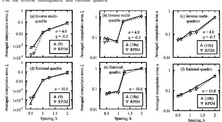
As a check of the performance of (9), (10a), and (10b), Figs. 5(a)…5(f) compare variation of interpolation errors with respect to different h values and two types of kernel functions.
Fig. 5(a)…5(f) ensures that (9), (10a), and (10b) are better applied using the inverse multiquadric and rational quadric kernel functions. In these six figures, (9), (10a), (10b) and the radial point interpolation method with polynomial reproduction interpolate (13) and its derivatives similarly accurately. At dense interpolation points (h = 0.5), Fig. 5(d) even indicates that (9), (10a), and (10b) interpolate u(x, y) more accurately.
Figs. 6(a)…6(c) depict variation of interpolation errors of u(x, y) with respect to coordinates x, y, and different γ values. Plotting these three figures adopts the rational quadratic kernel function, M = 441, and σ = 10.0.
Comparing Figs. 6(a)…6(c) finds that a large γ value can smooth interpolation errors generated using (9), (10a), and (10b). When the γ value increases from 1010 to 1012, these three figures indicate that interpolation errors decrease away from the point (0.4, 0.4). In addition, Figs. 6(a)…6(c) show that the interpolation error maximize at the point (0.4, 0.4).
Figure 6.Effects of nonzero γ values on interpolation errors (Using the rational quadric kernel function, M =441, σ = 10)
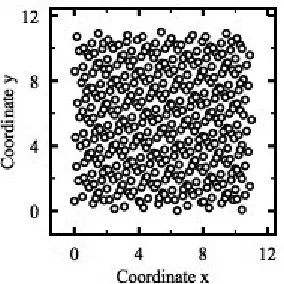
Figure 7.Randomly distributed interpolation points for estimating (13) and its derivatives
Table 3. Comparison of interpolation errors with respect to randomly located interpolation points shown in Fig. 7 (M = 441, γ = 1012)*
Averaged interpolation error
(9), (10a), and (10b)
Radial point interpolation method with polynomial reproduction
ξ 0.0001468 0.0006456
ζ 0.05822 0.05597
ε 0.055021 0.05333
Next, variation of averaged interpolation errors, ξ, ζ, and
ε under randomly distributed interpolation points are studied. Choose the case of M = 441 and add a two-dimensional Halton sequence to coordinates of interpolation points. Fig. 7 shows the new positions of interpolation points. Adopt these new positions of interpolation points to re-calculate ξ, ζ, and ε values. Table 3 lists the results of them. Editing this table uses the rational quadric kernel function, σ = 10.0, and γ = 1012.
Table 3 indicates that (9) interpolates u(x, y) more accurately but (10a) and (10b) interpolate its derivatives slightly inaccurately. But, considering that computing (9), (10a), and (10b) is time-saving, such ζ and ε values may be acceptable.
5. Conclusion
This study implements the minimum length method using new kernel functions, which come from the machine learning technique. In addition, a regularized minimum length method is created by considering the implementation
of it as a penalized least squares approximation problem; therefore, an error parameter is needed in interpolating a function. In the previous two sections, two interpolation experiments have competed to study variation of interpolation errors with respect to different required data. From these interpolation experiments, it is drawn:
(1) The performance of regularized minimum length method is comparable to the radial point interpolation method with polynomial reproduction. However, interpolating a function and its derivatives using this alternative scattered data interpolation method is time-saving.
(2) Inverse multiquadric and rational quadric kernel functions are two preferred kernel functions to implement the regularized minimum length method. Using these two types of kernel functions, obtaining sufficiently accurate interpolation results is expected.
(3) A large error parameter is effective in improving the instability of original minimum length method. It can smooth interpolation errors at some points. In conclusion, the proposed regularized minimum length method can be a useful scattered data interpolation method.
Nomenclature
B
0 = Collocation matrix.B = Kernel function. I = Identity matrix.
M = Total number of interpolation points.
N = Total number of points within a local support domain.
R = Radial basis function.
a, b = Unknown coefficients of the interpolation formula. c = Shape parameter.
dc = Characteristic length or averaged nodal spacing.
exact = Exact solutions.
h = Spacing between any two connecting interpolation points.
m = Total number of terms of a complete monomial basis.
num = Numerical solutions. p = A complete monomial basis. q = Shape parameter.
u = Function to be approximated. x, y = Spatial coordinates.
Ω = Local support domain.
Π = Lagrangian functional.
αc = Shape parameter.
ε = Averaged interpolation errors of the function derivative with respect to the y coordinate.
δ = Interpolation error.
γ = Error parameter for controlling interpolation errors.
λ = Lagrangian multiplier.
σ = Shape parameter.
ξ = Averaged interpolation errors of function values.
ζ = Averaged interpolation errors of the function derivative with respect to the x coordinate.
References
[1] M. D. Buhmann, Radial Basis Function: Theory and Implementation, New York: Cambridge, 2009, 272.
[2] W. Menke, Geophysical Data Analysis: Discrete Inverse Theory, 3rd ed., San Diego: Academic, 2012, 330.
[3] X. Liu, Q. Zhou, J. Birkholzer, and W. A. Illman, “Geostatistical reduced-order models in underdetermined inverse problems,” Water Resour. Res., vol. 49, iss. 10, pp. 6587-6600, October 2013.
[4] J. Kamm, Inversion and Joint Inversion of Electromagnetic and Potential Field Data, Ph. D. Thesis, Department of Earth Science, Uppsala University, Swedish, 2014, 108.
[5] G. R. Liu, K. Y. Dai, and H. Y. Li, “A meshfree minimum length method for 2-D problems,” Computat, Mech., vol. 38, iss. 6, pp. 533-550, November 2006.
[6] M. G. Genton, “Classes of kernels for machine learning: a statistics perspective,” J. Mach. Learn. Res., vol. 2, pp. 299-312, December 2001.
[7] C. Micchelli, “Interpolation of scattered data distance matrices and conditionally positive definite functions,” Constr. Approx., vol. 2, iss. 1, no. 1, pp. 11-22, December, 1986.
[8] E. Gilleland, Object Recogintion, Two-dimensional Kernel Smoothing: Using the R-package “smoothie” NCAR Technical Notes, National Center of Atmospheric Research, Colorado, USA, 24.
[9] G. F.. Fasshauer. Meshfree Approximation Methods with MATLAB, Singapore, World Scientific, 2007, 520.
[10] T. Evgeniou, M. Pontil, and T. Poggio, “Regularization networks and support vector machines,” Adv. Comput. Math. vol. 13, iss. 1, pp. 1-50, April 2000.
[11] F. Girosi, “An equivalence between sparse approximation and support vector machines,” Neural Comput. vol. 10, iss. 6, pp. 1455-1480, August 1998.
[12] J. A. Suykens, T. V. Gestel, J. D. Brabante, B. D. Moor, and J. A. Vandewalle. Least Squares Support Vector Machines, Singapore, World Scientific, 2002, 308.
[13] Y.-S. Xiong and D. Saad, “Noise, regularizers, and unrealizable scenarios in online learning from restricted training sets,” Phys. Rev. E, vol. 64, iss. 1, 011919, June 2001.
[14] K. V. Yuen. Bayesian Methods for Structural Dynamics and Civil Engineering, New York, Wiley, 2010, 320.