POD of vorticity fields: A method for spatial characterization of coherent structures

POD of vorticity fields: A method for spatial characterization

of coherent structures

Roi Gurka

, Alexander Liberzon

, Gad Hetsroni

a_{Department of Mechanical and Materials Engineering, University of Western Ontario, London, Canada} b_{Institute of Environmental Engineering, ETH Zurich, CH-8093 Zurich, Switzerland}

c

Faculty of Mechanical Engineering, Technion, Haifa 32000, Israel

Received 4 January 2005; received in revised form 23 December 2005; accepted 10 January 2006 Available online 6 March 2006

Abstract

We present a method to identify large scale coherent structures, in turbulent flows, and characterize them. The method is based on the linear combination of the proper orthogonal decomposition (POD) modes of vorticity. Spanwise vorticity is derived from the two-dimen-sional and two-component velocity fields measured by means of particle image velocimetry (PIV) in the streamwise–wall normal plane of a fully developed turbulent boundary layer in a flume. The identification method makes use of the whole data set simultaneously, through the two-point correlation tensor, providing a statistical description of the dominant coherent motions in a turbulent boundary layer. The identified pattern resembles an elongated, quasi-streamwise, vortical structure with streamwise length equal to the water height in the flume and inclined upwards in the streamwise–wall normal plane at angle of approximately 8.

2006 Elsevier Inc. All rights reserved.

PACS: 47.27.Nz; 47.54.+r

Keywords: Boundary layer; Vorticity; Proper orthogonal decomposition; Coherent structures; Identification

1. Introduction

Turbulent boundary layers have been extensively inves-tigated, since this is the place where the important phenom-ena of momentum and heat transfer, energy production and dissipation occur. One of the most important features in a turbulent boundary layer is the existence of coherent patterns (Kline et al., 1967; Panton, 1997). The role of coherent structures in the aforementioned phenomena, the interaction between the structures, and their relation to the properties of a turbulent flow, remain unclear (e.g., Tsinober, 2000). There is even no general consensus about

the geometry and the spatial characteristics of the coherent structures. Extensive experimental and numerical efforts were devoted to this problem during the past years ( Robin-son, 1991; Panton, 1997) and several models of the coher-ent structures were proposed, such as hairpin vortex packets (Zhou et al., 1999), horseshoe vortex (Theodorsen, 1952), funnel (Kaftori et al., 1994), and near-wall longitu-dinal vortices (Schoppa and Hussain, 2000), among others. Despite their different names, the spatial characteristics of the structures in all these models exhibit a remarkable sim-ilarity. For example, the individual coherent structures in the numerical simulations (e.g., Zhou et al., 1999) were found to grow upwards in the streamwise–wall normal plane at the angle of 8–12, as it was observed in the exper-iments of Head and Bandyopadhyay (1981) and Kaftori et al. (1994).

A study of coherent structures demands an objective, unbiased, statistical method of identification of the

coher-0142-727X/$ - see front matter 2006 Elsevier Inc. All rights reserved. doi:10.1016/j.ijheatfluidflow.2006.01.001

*

Corresponding author.

E-mail addresses:[email protected](R. Gurka),[email protected]. ethz.ch(A. Liberzon),[email protected](G. Hetsroni).

1 _{Tel.: +972 4 829 2058; fax: +972 48 23 8101.}

ent patterns in the multi-dimensional data sets. Numerous identification techniques have been proposed and imple-mented to the results of numerical simulations and experi-ments (see, for example Bonnet et al., 1998). The identification methods are associated with one of the phys-ically meaningful flow quantities, such as turbulent velocity or velocity derivatives. Vorticity, which plays a dominant role in the dynamics of turbulent flows (e.g., Klewicki, 1997; Tsinober, 2000), and linked directly to the coherent structures, is also one of the best choices for the identifica-tion (Bonnet et al., 1998; Gunes and Rist, 2004). We pro-posed in Liberzon et al. (2005) to use the linear combination of the proper orthogonal decomposition (Lumley, 1970) modes of the numerically simulated three-dimensional vorticity fields in order to identify and charac-terize the coherent structures in a turbulent channel flow. This method is distinct from the previous studies of the proper orthogonal decomposition (POD) (see reviews of Berkooz et al., 1993; Holmes et al., 1996), that have mostly analyzed velocity data, and have not used the combinations of POD modes in order to evaluate the spatial properties of the coherent structures.

In the present study we propose to use the same statisti-cal, unbiased characterization method, and in addition, uti-lize the recent developments of the particle image velocimetry (PIV) experimental technique (Adrian, 1991; Raffel et al., 1998). PIV provides measurements of the two-dimensional, two-component velocity fields with a spa-tial resolution, which is sufficiently high for the estimation of the out-of-plane component of vorticity. We apply our method to the ensemble of the instantaneous two-dimen-sional scalar fields of spanwise vorticity, experimentally obtained in a turbulent flow in a flume. The goal is to iden-tify the most essential features of the turbulent flow which are associated with high enstrophy, and characterize their geometry through the linear combination of the dominant POD modes.

Section2describes the flow facility and the PIV measur-ing system, along with the experimental results of the tur-bulent boundary layer. Section 3 is devoted to the presentation of the identification methodology and the dis-cussion of the characterization results. Section4comprises of some general remarks for conclusion.

2. The experiment

2.1. Experimental setup

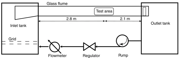
The experiment was performed in a flume with dimen-sions of 4.9·0.3·0.1 m, shown in Fig. 1. A detailed description of the flume is given in Liberzon et al. (2003) and Gurka et al. (2004), and here it is described only briefly. The entrance and the following part of the flume (up to 2.8 m downstream) are made of glass in order to make flow visualization and PIV measurements possible. All necessary precautions were taken to reproduce the same experimental conditions as in Hetsroni et al. (1997): (i) the eddies and recirculating currents were damped by means of grids in the inlet tank (as presented by dashed lines inFig. 1), (ii) baffles were installed in the pipe portion of the tank, the inlet to the channel was a converging chan-nel in order to have a smooth entrance, and (iii) the pump was isolated from the system by means of rubber joints fit-ted to the intake and discharge pipes. The pump was a 0.75 HP, 60 RPM centrifugal pump. Flowmeter, with an accu-racy of 0.5% of the measured flow rate, continuously recorded the flow rate. In order to make the measurement area long enough and avoid the flow depth decrease at the end of the flume, an array of cylinders restricted the flow before the outlet. The measurements have been performed with treated and filtered tap water.

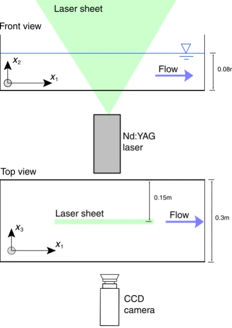
The PIV system, shown in Fig. 2, was composed of a double, pulsed, Nd:YAG laser (170 mJ/pulse, 15 Hz, 532 nm), optics for forming light sheet, and the CCD cam-era (8 bit, 1024·1024 pixels) with a recording rate of 30 frames-per-second. The camera was located 0.05 m from the side wall of the flume, normal to the laser light sheet formed in the mid-plane of the flume, measuring stream-wise and wall normal components of the velocity vector. Time separation between the two laser pulses was adjusted to 3 ms according to the free-stream streamwise velocity

U1= 0.21 m/s, and 150 successive velocity realizations were measured for the total time of 10 s. The Reynolds number, based on the flow heighth= 0.08 m and the kine-matic viscosity m= 0.8·106m2/s, was 21,000. Hollow glass spherical particles with an average diameter of 11lm, were used for seeding. The calibration procedure

Outlet tank Inlet tank

Grid

2.1 m 2.8 m

Test area

Pump Regulator

Flowmeter Glass flume

and PIV cross-correlation analysis were performed by using Insight 5.1 software, with 64·64 pixels interrogation areas and 50% overlapping. Spatial resolution of the cam-era was 80lm per pixel which provided a field of view of approximately 80·80 mm2. The analysis produced about 1000 vectors in each realization, filtered by using the stan-dard median and global outlier filters. During the post-pro-cessing analysis, 5% of the vectors were found to be erroneous. These vectors were removed and the gaps were filled with linear interpolations of the nearest neighbor points.

2.2. Experimental results

We measure the two-dimensional, two-component veloc-ity fields,~u1~u2in the streamwise–wall normal plane,x1–x2 (subscripts 1, 2 and 3 correspond to the streamwise, wall normal, and spanwise coordinates, respectively). Spanwise vorticity,x~3 is calculated through a numerical differentia-tion of the velocity fields. We denote the instantaneous fields with a tilde,~, the capital letters refer to the mean quantities, such as average vorticityX3¼xf3, the small let-ters denote the fluctuating fields (x3¼x~3X3), and the root-mean-square values are indicated by the apostrophe, for examplex0

3¼ ffiffiffiffiffiffi

x2 p

.

An example of the fluctuating velocity vector field {u1,u2} in the streamwise–wall normal (x1–x2) plane is shown as a vector plot in Fig. 3a. The abscissa is the streamwise coordinate,x1, and the ordinate is the wall nor-mal nornor-malized coordinate, x2, both normalized by the water heighth.

Despite the masking effect of the strong mean shear in the turbulent boundary layer on the underlying coher-ent structures, in the instantaneous fields we regularly observe the large patterns of concentrated vorticity, elon-gated in the streamwise direction and inclined upwards from the wall. These patterns represent, to the best of our understanding, the footprints of the large scale coher-ent structures, previously reported in the literature (e.g., Kaftori et al., 1994; Klewicki, 1997; Bonnet et al., 1998). An example of an instantaneous footprint of a structure could be seen in the contour plot of instantaneous vorticity field in Fig. 3b (we emphasize its envelope with a thick line).

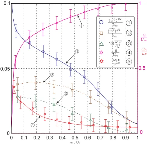
The statistical properties of the turbulent boundary layer are given inFig. 4. These include the profiles of the r.m.s. of velocity components, u0_{, v}0_{, (u=u}

1, v=u2) the Reynolds stressesuv, the mean streamwise velocity U (all normalized to the free-stream velocity,U1), and r.m.s. of spanwise vorticityx0

3, normalized by the friction velocity,

u*_{. The friction velocityu}*_{is estimated according to} Kaf-tori et al. (1994). The curves (1–4) (for the mean velocity and stresses) that refer to the results obtained byKlebanoff (1954)and reproduced inSchlichting (1979), are given for comparison. An additional curve (5) that shows the r.m.s. of spanwise vorticity is taken fromKim et al. (1987). Our results are presented by symbols and error bars. The sym-bols and the bars represent the average values and the uncertainty of the data, respectively.

0.25 0.5 0.75 1 1.25

0.05 m/s

0.05 0.15 0.25 0.35

x2

/h

x2

/h

x1/h

x1/h

0.25 0.5 0.75 1.0 1.25

0.05 0.15 0.25 0.35

-10 -5 0 5 10 15 20

3

w~

(a)

(b)

Fig. 3. Instantaneous flow fieldx1–x2plane: (a) velocity vector field and

(b) contours of the spanwise vorticityx~3. The flow is from left to right. Laser sheet

Laser sheet x

Flow

Flow Nd:YAG laser

2

x1

x1

x3

CCD camera Front view

Top view

0.3m 0.15m

0.08m

Fig. 2. Schematic drawing of the experimental setup. The measurement plane is the streamwise–wall normal plane,x1–x2, at the middle plane of

3. Characterization of vorticity fields

3.1. Methodology

In order to insure an objective identification process, we suggested in our previous work (Liberzon et al., 2005) to adopt the following guidelines:

• Data analysis has to be performed without threshold operations, and the same filters must be applied to all the data.

• Data has to be statistically significant in order to charac-terize the existing structures, over a period of time. • Analysis is based on a flow characteristic which strongly

represents turbulence.

The suggested method is, in some sense, a combination of the ‘‘characteristic eddy’’ concept ofLumley (1970)with the reconstruction technique which is similar to one pro-posed byGordeyev and Thomas (2002). The ‘‘large scale structure’’ or alternatively the ‘‘characteristic eddy’’ are identified through a linear combination of the dominant modes of the proper orthogonal decomposition (POD) of vorticity:

^

xiðxÞ ¼

XN

n¼1

an/niðxÞ i¼1;2;3; ð1Þ

where/n_iðxÞis an eigenfunction of ordernof the one of the components, denoted by subscripti. andenotes the

corre-sponding coefficient. An overview of the POD procedure and the way we apply it to the PIV results are given in Appendix A.

We infer that the proposed identification method, which is defined in the above expression (Eq. (1)) and which is using the rigorously proven optimal presentation through the POD, is an objective procedure and it satisfies the guidelines listed at the beginning of this section. Moreover, we show in the following that in addition to the identifica-tion, it also provides the spatial characterization of the coherent structures in turbulent flows.

3.2. Characterization and discussion

The analysis, based on the POD, has been implemented in certain types of flows, such as jets, boundary layers, backward facing step flows (e.g., Holmes et al., 1996; Gordeyev and Thomas, 2002). In most of the studies the fluctuating velocity fields were analyzed, assuming that the large-scale coherent structures contain the main frac-tion of the turbulent kinetic energy. However, it was noted in experimental studies ofKostas et al. (2001) and Liberzon et al. (2001)and shown in our recent study of the numeri-cally simulated flow (Liberzon et al., 2005), that the vortic-ity fields are more pertinent for the identification of coherent motions. This is mainly due to the fact that vortic-ity is Galilean invariant and, therefore, it is insensitive to the variations of the streamwise velocity that otherwise cause the so-called ‘‘jitter effect’’ and smear the boundaries of the coherent pattern.

We present a direct comparison of the vector POD modes of the instantaneous velocity, /u, with the scalar modes of spanwise vorticity, /_x3. In order to compare the vector fields with the scalar fields, we calculate the curl of the velocity POD mode and equate it with the POD mode of spanwise vorticity. In Fig. 5a the first velocity mode is shown as a vector plot, and its curl is specified by the contour lines. There is an evidence of a large scale Fig. 4. Mean profiles of turbulent stresses (i.e.,u0_,v0_{, andðuvÞ), and mean}

streamwise velocity U, all normalized by the free-stream streamwise velocity,U1, and r.m.s. of the spanwise vorticityx03, normalized by the

friction velocity,u*_{. Symbols and error bars represent the average and the}

variance of the data, respectively. For the comparison, the results of

Schlichting (1979), (1–4) and ofKim et al. (1987)(5) are shown as curves.

-0.06

-0.06 -0.06

-0.06

0.06 0.25 0.5 0.75 1.0 1.25

0.25 0.5 0.75 1.0 1.25 0.05

0.15 0.25 0.35

0.05 0.15 0.25 0.35

x2

/h

x2

/h

x1/h

(a)

(b)

pattern in Fig. 5a, which is elongated in the streamwise direction and inclined upwards in the streamwise–wall nor-mal plane. We observe this pattern, more clearly inFig. 5b, in which the boundaries of the pattern are less smeared out, it is easier identified in respect to the background vorticity and apparently also less contaminated with the noise. We infer that this is due to the weak influence of the streamwise velocity variations on vorticity, which is, by definition, a Galilean invariant.

In addition, inFig. 6we demonstrate that the 10 domi-nant POD modes of vorticity are sufficient for the recon-struction of any instantaneous vorticity field with a reasonable accuracy. The reconstruction means ‘‘partial reconstruction’’, defined in Appendix A (Eq.(9),K= 10). A relative error, based on the mean square difference between the original and the reconstructed fields, is also defined in Appendix A (Eq. (10)) and depicted in Fig. 7, along with the relative contributions of the single POD modes of spanwise vorticity. It is clear that the contribu-tion of the first modes is much higher than of the following, higher modes, and the relative error is below 8%. We also observe that the convergence of the cumulative contribu-tion of POD modes towards the 100% is relatively slow, as it was expected for the case of the small scale quantity, such as fluctuating vorticity (e.g., Liberzon et al., 2005).

The physical significance of vorticity in turbulent flows and the aforementioned technical details such as Galilean invariance, a sharper image and the small reconstruction error, are the main arguments for us to utilize vorticity eigenmodes in our identification method. Since a single POD mode of spanwise vorticity does not reproduce a coherent pattern typically observed in our measurements (e.g., Fig. 3b), we suggest to use the linear combination of the dominant POD modes in order to identify and char-acterize its spatial structure.

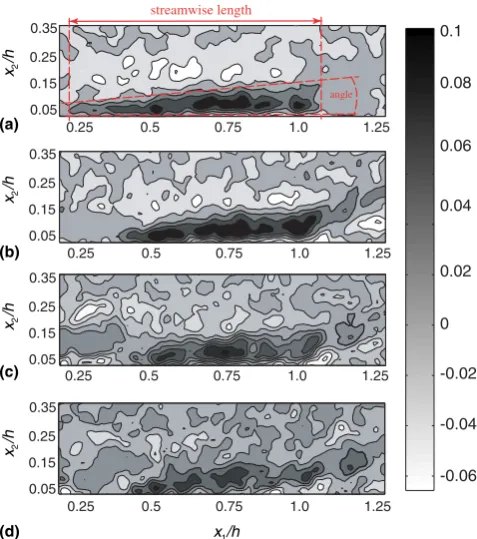
InFig. 8a–c we demonstrate the linear combinations of the 3, 5, and 10 dominant POD modes of spanwise

vortic-ity, respectively. For the sake of comparison we show the combination of all the available 150 modes in Fig. 8d. The ascertained picture inFig. 8a–d is of the streamwise-elongated pattern of concentrated vorticity (emphasized by a thick contour line). We also realize that the shape, the streamwise length and the inclination angle of this pat-tern, outlined inFig. 8a, have been not significantly altered by introducing the higher modes.

When the higher modes have been added to the linear combination, the pattern preserves its overall shape and

0.05 0.15 0.25 0.35

0.05 0.15 0.25 0.35

0.25 0.5 0.75 1.0 1.25

0.25 0.5 0.75 1.0 1.25

x2

/h

x2

/h

x1/h

x1/h

Fig. 6. Spanwise vorticityxe3 fields, original (top) and reconstructed by

means of 10 POD modes (bottom).

Fig. 7. Relative contribution of the single POD modes (dashed line), its cumulative summation (solid line) and relative errore(chain line), versus a number of POD modes.

-0.06 -0.04 -0.02 0 0.05

0.15 0.25 0.35 0.05 0.15 0.25 0.35

0.05 0.15 0.25 0.35

0.05 0.15 0.25 0.35

0.25 0.5 0.75 1.0 1.25

0.25 0.5 0.75 1.0 1.25

0.25 0.5 0.75 1.0 1.25

0.25 0.5 0.75 1.0 1.25

0.02 0.04 0.06 0.08 0.1

streamwise length

angle

x2

/h

x2

/h

x2

/h

x2

/h

x1/h

(d) (c) (b) (a)

geometry, but somewhat more details have been intro-duced. It is possible that the small regions of high vorticity, added to the large scale pattern, for example inFig. 8c, rep-resent the footprints of small-scale structures (e.g., hair-pins). However, since these dark zones change their shape when even more modes have been introduced, as for exam-ple inFig. 8d, it becomes less clear if the effect is due to the small scale structures or due to the noise introduced by the PIV technique. There is a possibility that some random noise from one of the PIV components (such as CCD cam-eras or non-uniform particle seeding density) or a bias error in the PIV algorithm (e.g., ‘‘peak locking effect’’, Raffel et al., 1998) bring in the small-scale features. Exper-imental data with much higher spatial and temporal resolu-tion is necessary in order to solve this ambiguity.

To summarize, we use the linear combination (defined in Eq. (1)) of the most dominant POD modes of spanwise vorticity (shown inFig. 8a) as an identification and charac-terization tool that provides a qualitative information, such as the shape of the coherent structures, and the quantitative information, such as the streamwise length and the inclina-tion angle of the coherent structures, in a turbulent bound-ary layer. The results shown in Fig. 8a–d emphasize the consistent spatial characteristics of the coherent patterns in the flow under investigation – the streamwise length, normalized by the water height is approximately equal to 1 and the typical inclination angle is roughly 8 in the streamwise–wall normal plane.

We can interpret the identified pattern as quasi-stream-wise vortical pattern, evolving from the wall towards the outer region of the boundary layer. Keeping in mind that the measured spanwise vorticity component,x3, is only a projection of the vorticity vectorx onto the x1–x2 plane, the pattern may be inferred as the footprint of an elongated quasi-streamwise vortical structure, which is growing to the sides (i.e., broadens) and upward from the wall. For example such a structure was entitled ‘‘funnel’’ in the exper-imental study ofKaftori et al. (1994), and it is also similar to the description of coherent structures disclosed by Schoppa and Hussain (2000) in a numerically simulated turbulent channel flow. The same type of the structure has been found also in our numerical investigation ( Liber-zon et al., 2005).

4. Concluding remarks

We present an experimental study of the large scale structures in a turbulent boundary layer in a flume. The two-component, two-dimensional velocity fields were mea-sured by means of particle image velocimetry (PIV). The footprints of the coherent structures were identified and spatially characterized through the identification method, previously applied to the numerically simulated vorticity vector fields inLiberzon et al. (2005).

The method is based on the proper orthogonal decom-position (POD) of vorticity and it explicitly fulfills the proposed guidelines for any objective and statistically

significant identification procedure: (i) the analysis uses an the whole data set, rather than a single flow field; (ii) it provides the spatial characteristics of a turbulent flow, on contrary to single-point statistics; (iii) it is not depen-dent on the choice of the basis functions (e.g., sinusoidal functions in Fourier transform, or wavelet basis), and (iv) it is based on a rigorous mathematically defined procedure of the proper orthogonal decomposition.

Based on the proposed methodology, the coherent pat-tern, as seen from the linear combination of the POD modes, is reflected through the spanwise vorticity compo-nent. This component is a projection of the vorticity vector, thus, we observe a footprint of an elongated quasi-streamwise vortical structure that emerge from the wall towards the mean flow and statistically have a length that is equal to the water height. The structure that we identify can be classified as a macro structure with a relative small inclination angle and is highly associated with the vorticity field. Note that the instantaneous velocity and vorticity maps do not present that feature in a repeatable manner nor does it appear in the mean values. Furthermore, decomposing the velocity fields will not yield the same result. Only by utilizing the technique on the vorticity field, a clear picture is revealed. Thus, the proposed meth-odology shows that coherent structures can be identified in turbulent boundary layers using two-dimensional, experi-mental data. In order to show a three-dimensional pattern, other fields of view in normal planes has to be measured, and three-dimensional data is necessary in order to educe the complete picture of the coherent structure. Neverthe-less, the presented method, which makes use of PIV results in a single plane, gives an additional insight into the spatial structure of the flow. It has been shown to assist evaluating the low-speed streaks (see for example Gurka et al., 2004) as well as the vortical structures (Liberzon et al., 2005).

Appendix A. Proper orthogonal decomposition (POD)

In this section the POD theory is discussed briefly and some key features of the implementation to the PIV data are presented.

POD was proposed by Lumley (1970) as an objective method to identify deterministic features in turbulent flows. The technique extracts different structures using orthogo-nal eigenfunctions of Karhunen–Loe´ve decomposition (Berkooz et al., 1993; Holmes et al., 1996). The empirical eigenfunctions are sometimes referred to ascoherent struc-tures, since they are highly correlated in an average sense with the flow field. In addition, the method was proved to be the optimal representation of the data (e.g.,Berkooz et al., 1993).

Z

Rðx;x0Þ/ðx0Þdx0¼k/ðxÞ; ð2Þ

where R(x,x0_{) is the two-point correlation matrix of} real-izations of the random field:

Rðx;x0Þ ¼ hfðxÞfðx0Þi. ð3Þ

The operator h i denotes ensemble average, and * de-notes complex conjugate. Eq.(2) has a finite set of eigen-functions f/ngN_n¼1 (N is the length of the realization vectors), called empirical eigenfunctions, proper orthogo-nal modes, or eigenmodes. The whole set of the modes is a complete orthogonal set, and allows the reconstruction of any member of the ensemble {fk} as follows:

fðxÞ ¼X

N

n¼1

an/nðxÞ; ð4Þ

where an are random uncorrelated coefficients that are

square roots of the eigenvalues:

hanami ¼

kn _n¼m;

0 otherwise.

ð5Þ

The amount of random field energy could be reproduced by the sum of the eigenvalues:

E¼ðf;fÞ ¼X

N

n¼1

kn; ð6Þ

where the operator (Æ,Æ) denotes the inner product

f;f

ð Þ ¼

Z

x

fðxÞfðxÞdx. ð7Þ

Notice that in the case of the turbulent velocity field (i.e.,

f(x) =u(x)),Eis twice the average turbulent kinetic energy of the flow. Thus, the magnitude of thenth eigenvalue kn

represents the average kinetic energy innth mode/n(x):

En_¼k

n

E. ð8Þ

In the same manner, in the case of the vorticity field

f(x) =x(x),Erepresents the average enstrophy of the flow, and each mode represents its contribution to the total ens-trophy (Liberzon et al., 2005).

It is possible to represent a low order model of the ran-dom field by reconstruction on the base of K dominant eigenmodes (usually the eigenvalues and eigenmodes are sorted in the ascending orderkn>kn+1):

^

fðxÞ ¼X

K

n¼1

an/nðxÞ. ð9Þ

The quality of the low-order model could be characterized by the error which is introduced by truncating the full ser-ies of the eigenmodes to the desired order. For example, we define the error of the approximation as a relative error:

e¼X

N

k¼1

ffiffiffiffiffiffiffiffiffiffiffiffiffiffiffiffiffiffiffiffiffiffiffiffiffiffiffiffiffiffiffiffiffi jfk_{ðxÞ f}^k_ðxÞj2

jfk_ðxÞj2

s

. ð10Þ

Sirovich (1987)proposed computationally efficient method ofsnapshots, which is used to compute the POD decompo-sition of the M snapshots (realizations) of size N, when

M<N, using the M·M symmetric matrix Rnm instead

of directly computed autocorrelation tensor:

Rnm¼

1

Mhf

n_fm_{i n;m¼1. . .M; ð11Þ}

which eigensolutions satisfy:

Rnmu¼ku ð12Þ

and from which the POD modes are calculated through the projection on the original fields

/n¼X

M

m¼1

un mf

m_{; ð13Þ}

where un

m is the mth element of the eigenvector u

corre-sponding to thenth eigenvaluekn.

The above derivation is valid for scalar functions f(x), such as the vorticity componentx3. For a vector-valued functions, such as the two-component velocity vector fields

u(x) = {u1,u2}, the tensorR(x,x0) is replaced by an ensem-ble averaged autocorrelation tensor R(x,x0_{) =hu(x)}

u(x0_{)iand the resulting POD modes are also vector valued.}

References

Adrian, R.J., 1991. Particle-imaging techniques for experimental fluid-mechanics. Ann. Rev. Fluid Mech. 23, 261–304.

Berkooz, G., Holmes, P., Lumley, J.L., 1993. The proper orthogonal decomposition in the analysis of turbulent flows. Ann. Rev. Fluid Mech. 25, 539–576.

Bonnet, J.P., Delville, J., Glauser, M.N., Antonia, R.A., Bisset, D.K., Cole, D.K., Fiedler, H.E., Garem, J.H., Hilberg, D., Jeong, J., Kevlahan, N.K.R., Ukeiley, L.S., Vincendeau, E., 1998. Collaborative testing of eddy structure identification methods in free turbulent shear flows. Exp. Fluids 25, 197–225.

Gordeyev, S., Thomas, F., 2002. Coherent structure in the turbulent planar jet. Part 2: Structural topology via POD eigenmode projection. J. Fluid Mech. 160, 349–380.

Gunes, H., Rist, U., 2004. Proper orthogonal decomposition reconstruc-tion of a transireconstruc-tional boundary layer with and without control. Phys. Fluids 16 (8), 2763–2784.

Gurka, R., Liberzon, A., Hetsroni, G., 2004. Characterization of turbulent flow in a flume with surfactant using PIV. ASME J. Fluids Eng. 126 (6), 1054–1057.

Head, M.R., Bandyopadhyay, P., 1981. New aspect of turbulent boundary layer structure. J. Fluid Mech. 107, 297–338.

Hetsroni, G., Zakin, J.L., Mosyak, A., 1997. Low-speed streaks in drag-reduced turbulent flow. Phys. Fluids 9, 2397–2404.

Holmes, P., Lumley, J.L., Berkooz, G., 1996. Turbulence, Coherent Structures, Dynamical Systems and Symmetry. Cambridge Mono-graphs on Mechanics. Cambridge University Press, Cambridge. Kaftori, D., Hetsroni, G., Banerjee, S., 1994. Funnel-shaped vortical

structure in wall turbulence. Phys. Fluids 6, 3035–3050.

Kim, J., Moin, P., Moser, R., 1987. Turbulence statistics in fully developed channel flow at low Reynolds number. J. Fluid Mech. 177, 133–166.

Klebanoff, P.S., 1954. Characteristics of turbulence in a boundary layer with zero pressure gradient. Technical Note 1247, NACA.

Kline, S.J., Reynolds, W.C., Schraub, F.A., Runstadler, P.W., 1967. The structure of turbulent boundary layers. J. Fluid Mech. 30, 741–773. Kostas, J., Soria, J., Chong, M.S., 2001. PIV measurements of a backward

facing step flow. In: Proc. 4th Intl. Symposium on Particle Image Velocimetry, Gottingen, Germany.

Liberzon, A., Gurka, R., Hetsroni, G., 2001. Vorticity characterization in a turbulent boundary layer using PIV and POD analysis. In: Proc. 4th Intl. Symposium on Particle Image Velocimetry, Gottingen, Germany. Liberzon, A., Gurka, R., Hetsroni, G., 2003. XPIV – multi-plane

stereoscopic particle image velocimetry. Exp. Fluids 36, 355–362. Liberzon, A., Gurka, R., Tiselj, I., Hetsroni, G., 2005. Spatial

character-ization of the numerically simulated vorticity fields of a flow in a flume. Theor. Comp. Fluid Dyn. 19 (2), 115–125.

Lumley, J.L., 1970. Stochastic Tools in Turbulence. Applied Mathematics and Mechanics, vol. 12. Academic Press, New York.

Panton, R.L., 1997. Self-Sustaining Mechanisms of Wall Turbu-lenceAdvances in Fluid Mechanics, vol. 15. Computational Mechanics Publications, Southampton, UK.

Raffel, M., Willert, C.E., Kompenhans, J., 1998. Particle Image Veloci-metry: A Practical Guide. Springer-Verlag, Berlin.

Robinson, S., 1991. Coherent motions in the turbulent boundary layer. Ann. Rev. Fluid Mech. 23, 601–639.

Schlichting, H., 1979. Boundary Layer Theory, seventh ed. McGraw-Hill, New York.

Schoppa, W., Hussain, F., 2000. Coherent structure dynamics in near-wall turbulence. Fluid Dyn Res 26, 119–139.

Sirovich, L., 1987. Turbulence and the dynamics of coherent structures. Part I: Coherent structures. Quart. Appl. Math. XLV, 561–571. Theodorsen, T., 1952. Mechanism of turbulence. In: Proc. 2nd

Midwest-ern Conference on Fluid Mechanics.

Tsinober, A., 2000. Vortex stretching versus production of strain/ dissipation. In: Hunt, J., Vassilicos, J. (Eds.), Turbulence Structure and Vortex Dynamics, Cambridge, pp. 164–191.