Evaluating the applicability of the finite element method for modelling of geoelectric fields

www.ann-geophys.net/31/1689/2013/ doi:10.5194/angeo-31-1689-2013

© Author(s) 2013. CC Attribution 3.0 License.

Annales

Geophysicae

Evaluating the applicability of the finite element method for

modelling of geoelectric fields

B. Dong1,2, D. W. Danskin2, R. J. Pirjola2,3, D. H. Boteler2, and Z. Z. Wang1

1_{Beijing Key Laboratory of High Voltage and EMC, North China Electric Power University, Beijing, China} 2_{Geomagnetic Laboratory, Natural Resources Canada, Ottawa, Canada}

3_{Finnish Meteorological Institute, Helsinki, Finland}

Correspondence to: B. Dong ([email protected])

Received: 2 April 2013 – Revised: 23 August 2013 – Accepted: 4 September 2013 – Published: 10 October 2013

Abstract. Geomagnetically induced currents in power sys-tems are due to space weather events which create geomag-netic disturbances accompanied by electric fields at the sur-face of the Earth. The purpose of this paper is to evaluate the use of the finite element method (FEM) to calculate the magnetic and electric fields to which long transmission lines of power systems on the Earth are exposed. The well-known technique of FEM is used for the first time to simulate mag-netic and electric fields applicable to power systems. Several test cases are modelled and compared with known solutions. It is shown that FEM is an effective modelling technique that can be applied to determine the electric fields which affect power systems. FEM enables an increased capability beyond the traditional methods for modelling electric and magnetic fields with layered earth conductivity structures, as spatially more complex structures can be considered using FEM. As an example results are presented for induction, due to a line current source, in adjacent regions with different layered con-ductivity structures. The results show the electric field away from the interface is the same as calculated for a single re-gion; however near the interface the electric field is influ-enced by both regions.

Keywords. Electromagnetics (Numerical methods) – Geo-magnetism and paleoGeo-magnetism (Geomagnetic induction) – Ionosphere (Electric fields and currents)

1 Introduction

During geomagnetic disturbances, the changing mag-netic field produces an electric field that drives large electric currents in power transmission networks. These

geomagnetically induced currents (GIC) can cause a vari-ety of problems for operation of power transmission systems (Boteler et al., 1998; Molinski, 2002; Pirjola et al., 2004). Traditionally this has been considered a problem for high-latitude power systems, however in recent years, GIC have been found in power systems of some mid- or low-latitude countries such as Japan (Kappenman, 2003), Brazil (Pinto et al., 2004; Trivedi et al., 2007), South Africa (Koen and Gaunt, 2003; Gaunt and Coetzee, 2007) and China (Liu et al., 2009). A notable example of GIC was the March 1989 magnetic storm that affected power systems in North Amer-ica and Europe (Kappenman, 1996; Bolduc, 2002).

Modelling of GIC in power systems consists of two parts (e.g. Viljanen and Pirjola, 1994). The first step is to obtain the electric field at the surface of the Earth taking the Earth’s con-ductivity structure into account (e.g. Hakkinen and Pirjola, 1986). The second step is calculation of GIC based on the power system’s physical layout and resistances and the elec-tric field such as discussed for the benchmark case (Horton et al., 2012). One of the largest problems is how to estimate the electric field to which a power transmission network will be exposed. This is straightforward for source fields that can be modelled as a “plane wave” and assuming a laterally uniform earth that can be represented by a layered-earth conductivity model. However, calculating the electric fields for more real-istic situations involving lateral variations in both the source fields and the earth conductivity is considerably more diffi-cult.

even more complicated ionospheric currents. Boteler and Pirjola (1998) implemented a complex image method (CIM) (Thomson and Weaver, 1975) to approximately evaluate this field for layered earth models of conductivity in an efficient manner. The Fast Hankel Transform (FHT) method can be used to calculate the integrals that give exact expressions for the electric and magnetic fields at the surface of an uniform or layered earth due to an overhead line current (Johansen and Sorensen, 1979; Pirjola, 1985). This method was used by Zheng et al. (2013) to look at the effects of magnetospheric and ionospheric currents on the surface impedance.

To model lateral variations in the earth conductivity ture requires techniques that can handle 2-D or 3-D struc-tures. The finite element method (FEM) has been used in the past to study induction and resistivity problems (Coggon, 1971; Reddy and Rankin, 1975; Reddy et al., 1977; Pridmore et al., 1981). The main focus of these papers was to evalu-ate what type of conductivity structures of the Earth could be modelled. If the conductivity structure is assumed to be known, the electric and magnetic fields in the Earth can also be determined by this method.

In this paper, the FEM technique is used to study induction due to a line current source with different earth conductiv-ity structures. First, the technique is evaluated to show that it is applicable to calculate the electric and magnetic fields in connection with GIC studies. Cases of a line current in free space, or with uniform and layered earth conductivity structures are compared with results from analytical or FHT solutions to verify the results. Finally, cases of laterally non-uniform layered earth models are considered to show the new results associated with the surface impedance that can be obtained with the FEM technique. These cases also show how the source and the earth structure influence the surface impedance calculations related to the electric fields that drive GIC in power systems.

2 The finite element method

The finite element method (FEM) originated from structural engineering in the 1960s and is now used in studies of a variety of engineering problems, e.g. structural, heat trans-fer, computational fluid dynamics and electromagnetism. FEM is a numerical method for solving complex differen-tial equations subject to boundary conditions. In electromag-netic applications, the method is suited to model arbitrary distributions of conductivity in three-dimensional problems by using the Galerkin method of weighted residuals (Fin-layson, 1972). In this method, a linear combination of ap-proximation functions and coefficients is used to decompose the electromagnetic fields or potentials over finite elements (Zienkiewicz, 1971).

The advantage of introducing potentials is that the total number of the degrees of freedom can be reduced. The elec-tric and magnetic fields can be expressed in terms of the

scalar potential and the vector potential. The divergence of the vector potential is chosen to be zero. In all cases where the direction of the gradient of the conductivity is perpendic-ular to the electric field, the divergence of the electric field is zero resulting in no charge accumulation.

A Cartesian coordinate system is used, following the ge-omagnetic convention, wherex is northward,yis eastward, andz is vertically down. All structures are assumed to be uniform in they direction and to extend to infinity in they direction. The source current is in the positiveydirection re-sulting in the vector potential only having aycomponent and the gradient of the scalar potential is zero due to the uniform structure along theydirection. The governing equation in the examples in this paper is Poisson’s equation for the magnetic vector potential (Eq. 1), when the current is considered only in one direction (y).

−1 µ∇

2_A

y+j ωσ Ay=Js (1)

Jsis the source current density andAyis the magnetic vector

potential.ωis the angular frequency,µandσare the perme-ability and the conductivity of the region.σequals zero in the air region and has conductivity values in the Earth. Apply-ing Galerkin finite element method to Eq. (1), the governApply-ing equation can be written as (Zienkiewicz, 1971):

np X

n=1

"_n e X

e=1

Z ₁

µ∇Mm· ∇Mn+MmMnj ωσ

d #

Ayn

=

ne X

e=1

Z

(MmJs)d; (2)

m=1, 2, 3, . . . ,np.

TheMmare the weighting functions and theMnare the

ba-sis functions.npandneare the total number of nodal points

and elements, respectively. The weighting functions and ba-sis functions in the elementesatisfyMm=NiandMn=Nj,

whereNi andNj are the shape functions andi, j=1, 2, 3,

. . . ,n. Here n denotes the total number of nodal points in each element and can be variable due to different types of ele-ments. This can result in a large number of integral equations for large mesh structures which must be solved resulting in increased computational memory and time.

The global coordinate system (x, z) is transformed by isoparametric coordinate transformation to the natural coor-dinate system (ξ,η). The shape functions at each nodal point of the rectangular element in the natural coordinate system are:

Ni(ξ, η)=

1

4(1+ξiξ ) (1+ηiη); (3)

i=1, 2, 3, 4.

Substituting Eq. (3) into Eq. (2) can simplify the inte-gration procedure and the magnetic vector potential at each nodal point can be solved.

For this paper, the ANSYS version 5.7 software (http: //www.ansys.com/) is used for the two dimensional simula-tions. Since the exact implementation within the FEM code to solve these problems is not known, the FEM results of test cases are compared with known solutions from analyt-ical techniques to give confidence in FEM. The highly de-tailed equations within the FEM software can be found in the manual of the software (http://research.me.udel.edu/~lwang/ teaching/MEx81/ansys56manual.pdf).

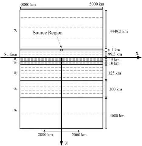
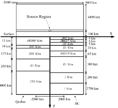
Initially, the source current is set to be a line current at a height of 100 km as done by Hermance and Peltier (1970) with the magnitude 106A, and is represented as a current density with the magnitude 1 A m−2in a 1 km×1 km square cross-sectional area. The layout of the physical model and computational model are shown in Fig. 1. The thin layer of 1 km thickness with its center at a height of 100 km is the source region where either a line current or wide current can be placed. The scale of the physical model is chosen as large as possible to ensure the magnetic fields in thexandz direc-tions attenuate to zero at the boundaries. Thus, the depth of the physical model should be chosen to extend sufficiently far below the Earth’s surface. The dashed lines in Fig. 1 indicate that the physical layers will be divided into several layers of elements for computation.

In the computational model, the element density is chosen to be sufficiently high in regions where accurate values are to be evaluated. Lower element densities can be used for re-gions far displaced from the region of interest. The electric and magnetic fields at the Earth surface and under the surface are most important in these computations, so a computational horizontal scale between−2000 km and 2000 km with a res-olution of 1 km is chosen. The top three conductivity layers of the Earth have a resolution of 1 km, whereas the lower two layers have 20 km and 2000 km resolutions. In the air region, the layers above and below the current are divided into ten layers.

The rectangular computational grid is used in the simula-tions for a free space case and for cases involving uniform and layered earth conductivity structures. The FEM values are computed at the centre of each rectangular cell by aver-aging the values at the nodes. The horizontal resolution of 1 km was chosen such that the values are in agreement with the analytical results for the free space case as described in the following section. The model is designed so that the elec-tric field is only in the y direction, with the magnetic field in thex andzdirections. The time period can be varied with initial comparisons done at a period of 300 s.

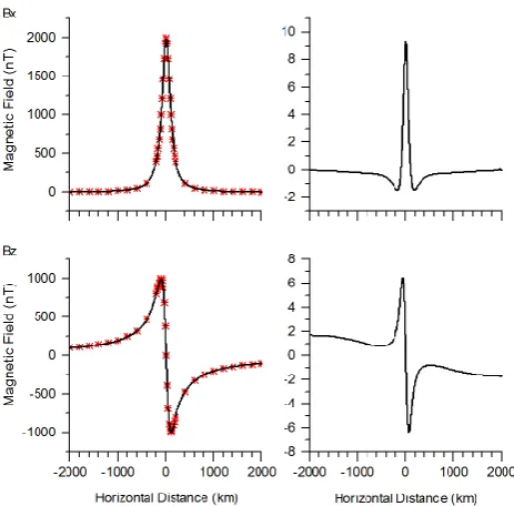
2.1 Free space case

To test that the boundary conditions for the FEM model are correct, a simple case of a line current flowing in free space is considered. In this case, the magnetic field has a well known analytical solution given by Ampere’s Law. In Fig. 2, the cal-culated magnetic field at the (fictitious) Earth’s surface from

1

Figure 1.

Sketch of the physical and computational model used for evaluation of electric and

2

magnetic fields. The dashed horizontal lines represent computational boundaries whereas the

3

solid lines are physical boundaries. A large physical model is necessary to satisfy the

4

boundary conditions of the magnetic field being sufficiently attenuated. The conductivities

5

and thicknesses of the different layers can be varied depending on the layered Earth model. A

6

current is placed at 100 km above the surface in a thin 1-km layer. The computational

7

gridding of 1 km in the x dimension is omitted for clarity. For the Quebec layered earth

8

model, σ

= .00005 S/m, σ

= .005 S/m, σ

= .001 S/m, σ

= .01 S/m and σ

= .333 S/m, and

9

the layer thicknesses are shown in the figure.

10

Fig. 1. Sketch of the physical and computational model used for

evaluation of electric and magnetic fields. The dashed horizontal lines represent computational boundaries whereas the solid lines are physical boundaries. A large physical model is necessary to sat-isfy the boundary conditions of the magnetic field being sufficiently attenuated. The conductivities and thicknesses of the different lay-ers can be varied depending on the layered Earth model. A cur-rent is placed at 100 km above the surface in a thin 1 km layer. The computational gridding of 1 km in thexdimension is omitted for clarity. For the Quebec layered earth model,σ1=0.00005 S m−1,

σ2=0.005 S m−1,σ3=00.001 S m−1,σ4=0.01 S m−1andσ5=

0.333 S m−1, and the layer thicknesses are shown in the figure.

16 1

Figure 2. The magnetic field components at z=0 and their differences from theoretical values

2

for the free space case. The red symbols are the exact solution and the black line is the FEM 3

solution. The graphs in the right column are the difference between the exact solution and the 4

FEM model. The period is 300 s. 5

6

Fig. 2. The magnetic field components atz=0 and their differences from theoretical values for the free space case. The red symbols are the exact solution and the black line is the FEM solution. The graphs in the right column are the difference between the exact solution and the FEM model. The period is 300 s.

The free space case highlights the system of magnetic fields that would be expected from this type of simulation. The magnetic field has bothx andzcomponents. The peak value of thex component (2000 nT) occurs directly beneath the line current whereas thezcomponent has a value of zero below the line current. Thezcomponent has positive values for negativexand negative values for positivex, with largest magnitudes (1000 nT) at approximately±100 km. Now that the framework is set up, changes to the magnetic field can be noted as the conductivity structure is modified.

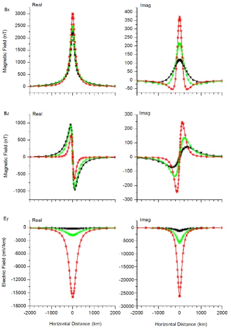
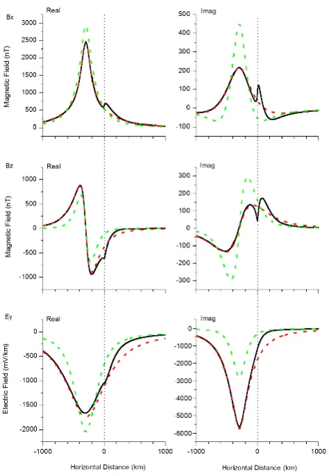
2.2 Uniform Earth

In this case all the layers below the surface of the Earth are set to a conductivity value of 0.001 S m−1and calculations are made for a period of 300 s. In Fig. 3, the FEM results are shown as solid lines and for comparison the results based on the Fast Hankel Transform (FHT) are shown as symbols. The FHT method gives results at the surface (z=0) for both a layered earth and uniform earth cases.

Each of the magnetic field and electric field components now has a complex value. Visually, it can be seen that the magnetic fields of FHT and FEM agree to within 1 %. For the electric field, the imaginary part is more than twice that of the real part, whereas the magnetic fields components still retain much larger real parts than imaginary parts.

One clear difference is that the maximum value of the horizontal component of the magnetic field is approximately 2500 nT compared with the 2000 nT value in the free space

17 1

Figure 3. The electric and magnetic field components at the surface for an uniform Earth with 2

a conductivity of 0.001 S/m. The FEM results are the black curve whereas the FHT results 3

are the red symbols. The period is 300 s. 4

Fig. 3. The electric and magnetic field components at the surface

for an uniform Earth with a conductivity of 0.001 S m−1. The FEM results are the black curve whereas the FHT results are the red sym-bols. The period is 300 s.

case. The presence of the conducting Earth has increased the value of the horizontal magnetic field. This is because the magnetic field occurring on the surface of the Earth is a com-bination of both the direct magnetic field from the line cur-rent and the magnetic field from induced curcur-rents below the surface.

2.3 Layered Earth

As another test, calculations are made for a layered Earth conductivity structure. For this comparison the Quebec model discussed by Boteler and Pirjola (1998) and shown in Fig. 1 is used in the simulation results that are presented in Fig. 4. Once again FEM is the solid lines and FHT is the symbols. In general the results are identical to within 1 %.

By varying the time period, the frequency response of the system can be evaluated. For long periods (i.e. 1800 s or 30 min), the system is responding more like the free space case, with the electric field being substantially suppressed

18 1

Figure 4. The electric and magnetic field components at the Earth’s surface are shown for the 2

layered earth conductivity model of Quebec. The FEM results are the solid curves whereas 3

the FHT results are symbols. The colours of the curves represent the periods with red being 4

30 s, green being 300 s and black being 1800 s. 5

6

Fig. 4. The electric and magnetic field components at the Earth’s

surface are shown for the layered earth conductivity model of Que-bec. The FEM results are the solid curves whereas the FHT results are symbols. The colours of the curves represent the periods with red being 30 s, green being 300 s and black being 1800 s.

and the magnetic field becoming almost purely real and tend-ing to 2000 nT for Bx and 1000 nT for Bz at the maxima.

For the short period case (30 s), both the real and imag-inary parts of Bx increase, whereas the real part of Bz is reduced while the imaginary part increases. For the electric field, both the real and the imaginary parts are substantially increased compared with the longer period cases.

3 Discussion

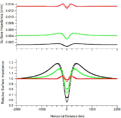
Much of the modelling efforts associated with GIC re-search have been designed to be able to compute the sur-face impedance that can be used with recorded magnetic field variations to calculate the electric fields experienced by a power system. The surface impedance is defined as: Z=µ0E/B, whereEandBare orthogonal components of

the horizontal electric and magnetic fields at the surface of the Earth. In Fig. 5, the magnitude of the surface impedance

1

Figure 5. The magnitude of surface impedance for the layered earth conductivity model of

2

Quebec is shown for three different periods (red 30s, green 300s, and black 1800s). The FEM

3

results are the solid curves whereas the FHT results are symbols. The lower graph shows the

4

relative impedance based on FEM where each value is normalized by the value at x = -2000

5

km.

6

7

Fig. 5. The magnitude of surface impedance for the layered earth

conductivity model of Quebec is shown for three different periods (red 30 s, green 300 s, and black 1800 s). The FEM results are the solid curves whereas the FHT results are symbols. The lower graph shows the relative impedance based on FEM where each value is normalized by the value atx= −2000 km.

computed for the Quebec layered earth case is shown. The FEM (solid line) and FHT (symbols) results agree very well to within 0.5 %. For large values ofx, the surface impedance tends to the plane wave value as pointed out by Zheng et al. (2013). The surface impedance increases as the period de-creases, which results in the higher frequency components of the electric spectrum being enhanced relative to the magnetic spectrum.

Beneath the line current source, the surface impedance changes due to the fields from the line current not being suf-ficiently planar (e.g. Viljanen et al., 1993, 1999). To further illustrate this point, in the lower part of Fig. 5, the surface impedance for each frequency is normalized by dividing by the plane wave impedance. This shows that the relative sur-face impedance can vary substantially from 0.55 to 1.30 in the region between −2000 km and 2000 km for the 1800 s period. At a period of 300 s the range of variation is reduced to 0.72 to 1.20. At the shortest period (30 s), the range of variation is much less (0.9 to 1.1) and is much more local-ized between−400 km and 400 km.

Now with the FEM framework established, further prob-lems can be studied. Consider the problem of a wide current of 200 km width centred 100 km above the earth overx=0. To simplify the comparison, the total current is still set to 1 MA. In Fig. 6 the magnitude of the surface impedances for a wide current (symbols) are compared with those for a line current (solid lines) for the periods of 30 (red), 300

20

1

Figure 6. The magnitude of the surface impedance for a layered earth conductivity model of

2

Quebec is shown for three different periods for a 1 km line current (solid) and a 200 km wide

3

current (symbols). The colours of the curves represent the periods (black 1800 s, green 300 s

4

and red 30 s). The lower graph shows the relative impedance where each value is normalized

5

by the value at x = -2000 km. The computations are based on FEM.

6

Fig. 6. The magnitude of the surface impedance for a layered earth

conductivity model of Quebec is shown for three different periods for a 1 km line current (solid) and a 200 km wide current (symbols). The colours of the curves represent the periods (black 1800 s, green 300 s and red 30 s). The lower graph shows the relative impedance where each value is normalized by the value atx= −2000 km. The computations are based on FEM.

(green) and 1800 (black) seconds. A wide current generates fields that are similar, but the impedance variations are broad-ened and not as extreme. For the long period case (black lines and symbols), the relative impedance depression is less-ened directly below the wide current between+100 km and −100 km, but it is enhanced between 100 and 400 km. The effects of the relative surface impedance at further distance are still the same as those of the simple line current.

The FEM modelling also provides the opportunity to see how the fields vary with depth within the Earth; a capability not present with FHT. Figure 7 shows results obtained with the Quebec conductivity structure, featuring vertical slices taken through the layered Earth at several different positions along thex direction for each of the components for a pe-riod of 300 s. The curves of Fig. 7 have been transformed into magnitude and phase to show clearly how the fields at-tenuate with increasing depth. The black lines show how the fields vary with depth directly below the line current. The blue dot-dashed line is at+100 km near the maximum of the vertical component of the magnetic field. The red line is at+800 km and illustrates how the horizontal component of the magnetic field is approaching zero. The green dot-dashed line is at+1500 km and shows how all the fields have very small values. The conductivity values of the layers are vary-ing from a low conductivity of 0.00005 S m−1for the first, to a significantly larger value of 0.005 S m−1for the second

21

1

Figure 7. The magnitude and phase variations of the electric and magnetic fields with depth

2

at x=0 (black), x=100 (blue dot-dashed), x=800 (red) and x=1500 km (green dot-dashed) for a

3

layered earth conductivity model of Quebec are shown for a 1 km line current located at x =0,

4

100 km above the surface and having a period of 300 s. The computations are based on FEM.

5

6

7

Fig. 7. The magnitude and phase variations of the electric and

mag-netic fields with depth atx=0 (black),x=100 (blue dot-dashed),

x=800 (red) andx=1500 km (green dot-dashed) for a layered earth conductivity model of Quebec are shown for a 1 km line cur-rent located atx=0, 100 km above the surface and having a period of 300 s. The computations are based on FEM.

and a conductivity 0.001 S m−1for the third layer. The layer transitions (marked by dashed lines in the upper two panels) are clearly observed in both the magnitude and the phase of the x component of the magnetic field especially near the source region (black and blue dot-dashed curves). Clearly, the ability to examine the changes of the fields with depth is enhanced by using FEM.

The FEM technique can also be used to model complex conductivity structures of the Earth as shown in Fig. 8 where there is an interface region between two layered earth struc-tures. In this model the layered earth structure of Quebec is used for x< 0 and the layered earth structure of British Columbia (BC) is used forx> 0. Figure 9 shows the results of the FEM simulation for a line current source placed 100 km above the interface region atx= 0. The black curve is for the combined case with the two different layered earth struc-tures (see Fig. 8). For comparison, the red curve is for the case of the Quebec layered earth structure, assuming that the

1

Figure 8. The combined earth model is used for the evaluation of electric and magnetic fields.

2

For x < 0 the Quebec layered earth model is used. For x > 0 the British Columbia layered

3

earth model is used. The conductivities and thicknesses of the different layers are shown. A

4

current is placed at 100 km above the surface in a thin 1-km layer.

5

Fig. 8. The combined earth model is used for the evaluation of

elec-tric and magnetic fields. Forx< 0 the Quebec layered earth model is used. Forx> 0 the British Columbia layered earth model is used. The conductivities and thicknesses of the different layers are shown. A current is placed at 100 km above the surface in a thin 1 km layer.

conductivity profile is the same for both positive and negative x. Using this same assumption, the green curve represents the results for the BC layered earth structure. Clearly it is shown that at large distances from the interface, the fields with the combined model tend to the same values as the fields for the Quebec or BC model on their respective sides of the inter-face. The Quebec structure represents a highly resistive struc-ture whereas the BC strucstruc-ture represents a more conductive structure. The most significant feature is that the fields are no longer symmetric with respect to the location of the line current source. The electric field maximizes on the Quebec side whereas the magnetic field maximizes on the BC side. In the interface region the combined model does not seem to be just the linear superposition or average of the two mod-els. For the BC side, the fields become similar after 100 km from the interface but for the Quebec side, the fields do not become similar until at least 500 km.

To check how the fields are affected by the location of the source, model calculations are made of the fields produced by line currents on either side of the interface. Figure 10 shows the results for the simulation when the line current is moved 300 km to the Quebec side from the interface. The combined results agree with Quebec model results further than 100 km from the interface, and with the BC model re-sults further than 300 km from the interface. Clearly near the interface region, the fields with the combined model are not the same as the fields produced by either individual model. Figure 11 shows simulation results for the line current lo-cated 300km to the BC side from the interface. It is seen that

23 1

Figure 9. The electric and magnetic field components at the Earth’s surface are shown for 2

three different cases. The red curves represent the results with the Quebec layered earth 3

model, the green curves represent the results with the BC layered earth model and the black 4

curves represent the results with the combination of the layered earth structure of Quebec for 5

x < 0 and the layered earth structure of BC for x > 0 (see Fig. 8). The line current is located 6

100 km above the x = 0 point which is the interface between the Quebec structure and the BC 7

structure. The computations are based on FEM with a period of 300 s. 8

Fig. 9. The electric and magnetic field components at the Earth’s

surface are shown for three different cases. The red curves rep-resent the results with the Quebec layered earth model, the green curves represent the results with the BC layered earth model and the black curves represent the results with the combination of the layered earth structure of Quebec forx< 0 and the layered earth structure of BC forx> 0 (see Fig. 8). The line current is located 100 km above thex= 0 point, which is the interface between the Quebec structure and the BC structure. The computations are based on FEM with a period of 300 s.

the combined results are the same as with the BC model for distances greater than 100 km from the interface. The fields with the combined model are different from those with the Quebec model until at least 500 km from the interface. Once again the fields near the interface region are not the same as the fields produced by either individual model.

24 1

Figure 10. Same as Fig. 9 but the line current is displaced from the interface region to x = -2

300 km. 3

4

Fig. 10. Same as Fig. 9 but the line current is displaced from the

interface region tox= −300 km.

4 Conclusions

In this paper, the well-known technique of FEM was used for the first time to calculate magnetic fields and associated electric fields that could drive GIC in power systems. It has been demonstrated that the results from FEM and the results of analytical expressions or FHT calculations are identical to within 1 %, when a sufficiently large model was chosen for FEM with a sufficiently good resolution of elements. FEM can be considered for problems that have no simple physical layout or where the mathematical equations are too difficult to solve in practice. In addition FEM gives the values below the surface of the Earth and not just at the Earth’s surface. The advantage of the FEM toolkit is that once the physical and computational models are established then parameters can be adjusted to give solutions for similar problems. FEM is capable of calculating the fields below the surface of the earth without the need to derive complex mathematical ex-pressions. FEM can be further used for complicated current systems and/or spatially varying conductivity models.

One of the limitations of FEM is that the amount of com-putational power increases with the complexity of the layered

25 1

Figure 11. Same as Fig. 9 but the line current is displaced from the interface region to x = 2

300 km. 3

4

Fig. 11. Same as Fig. 9 but the line current is displaced from the

interface region tox=300 km.

26

1

Figure 12. The surface impedances for the combined models of the three different cases of

2

Fig. 9 – 11. The black curve is the surface impedance when the line current is located above

3

the interface region. The red curve is the surface impedance when the line current is located

4

at -300 km and the green curve is the surface impedance when the line current is located at

5

300 km. The computations are based on FEM with a period of 300 s.

6

Fig. 12. The surface impedances for the combined models of the

three different cases of Figs. 9–11. The black curve is the surface impedance when the line current is located above the interface re-gion. The red curve is the surface impedance when the line current is located at−300 km and the green curve is the surface impedance when the line current is located at 300 km. The computations are based on FEM with a period of 300 s.

earth structures. In three-dimensional FEM, the simulations still have to be run on a supercomputer. For simple cases such as free space case, it is computationally more efficient to use

analytical solutions or other codes such as FHT. As the com-plexity of the problem increases, the advantage of FEM is demonstrated.

The FEM technique was used to estimate the surface impedance of both line currents and wide currents. The FEM values for the electric field and the magnetic field can be used directly to calculate the surface impedance. Also, FEM prop-erly handles situations of regions close to the source so the assumption of a plane wave source is not necessary.

FEM was used to evaluate a more complex model prised of two different layered models and shows the com-plexity of the surface impedance in the interface region be-tween the two structures. The variations of the fields in the interface region are of prime interest to GIC researchers. This paper shows the value of using FEM in GIC studies and im-portant new results for the surface impedance, commonly used in GIC modelling.

Using FEM, a wide variety of physical systems with dif-ferent input sources can be simulated in a very short period of time. Computational time for each of the simulations is less than 10 min on a typical laptop computer. In future work, FEM will be used to investigate the effects of boundaries be-tween layered conductivity blocks of the Earth, in particular the “coast effect” at the ocean-land interface emphasising ap-plications to GIC research.

Acknowledgements. The funding for B. Dong was supported by the

Program of the Co-Construction with Beijing Municipal Commis-sion of Education of China (GJ20120006) and the National Na-ture Science Foundation of China (51177045). The authors thank C. M. Liu and L. Trichtchenko for useful discussions leading to this research.

Topical Editor K. Hosokawa thanks P. J. Cilliers and one anony-mous referee for their help in evaluating this paper.

References

Bolduc, L.: GIC observations and studies in the Hydro-Quebec power system, J. Atmos. Sol.-Terr. Phy., 64, 1793–1802, 2002. Boteler, D. H. and Pirjola, R. J.: The complex-image method for

calculating the magnetic and electric fields produced at the sur-face of the Earth by the auroral electrojet, Geophys. J. Int., 132, 31–40, 1998.

Boteler, D. H., Pirjola, R., and Nevanlinna, H.: The effects of ge-omagnetic disturbances on electrical systems at the Earth’s sur-face, Adv. Space Res., 22, 17–27, 1998.

Coggon, J. H.: Electromagnetic and electrical modeling by the finite-element method, Geophysics, 36, 132–155, 1971. Finlayson, B. A.: The method of weighted residuals and variational

principles, Academic Press, New York, 1972.

Gaunt, C. T. and Coetzee, G.: Transformer failure in regions incor-rectly considered to have low GIC-risks, in 2007 IEEE Lausanne Power Tech, 807–812, Inst. of Electr. and Electr. Eng., New York, 2007.

Hakkinen, L. and Pirjola, R.: Calculation of electric and magnetic fields due to an electrojet current system above a layered earth, Geophysica, 22, 31–44, 1986.

Hermance, J. F. and Peltier, W. R.: Magnetotelluric fields of a line current, J. Geophys. Res., 75, 3351–3356, 1970.

Horton, R., Boteler, D., Overbye, T. J., Pirjola, R., and Dugan, R. C.: A test case for the calculation of geomagnetically induced currents, IEEE T. Power Deliver., 27, 2368–2373, 2012. Johansen, H. K. and Sorensen, K.: Fast Hankel Transforms,

Geo-phys. Prospect., 27, 876–901, 1979.

Kappenman, J. G.: Geomagnetic Storms and Their Impact on Power Systems, IEEE Power Engineering Review, May 1996, 5–8, 1996.

Kappenman, J. G.: Storm sudden commencement events and the associated geomagnetically induced current risks to ground-based systems at low-latitude and midlatitude locations, Space Weather, 1, 1016, doi:10.1029/2003SW000009, 2003.

Koen, J. and Gaunt, T.: Geomagnetically induced current in the Southern African electricity transmission network, unpublished, presented at 2003 IEEE Bologna PowerTech Conference, 2003. Liu, C. M., Liu, L. G., and Pirjola, R.: Geomagnetically induced

currents in the high-voltage power gird in China, IEEE T. Power Deliver., 24, 2368–2374, 2009.

Molinski, T. S.: Why utilities respect geomagnetically induced cur-rents, J. Atmos. Sol.-Terr. Phy., 64, 1765–1778, 2002.

Peltier, W. R. and Hermance, J. F.: Magnetotelluric fields of a Gaus-sian electrojet, Can. J. Earth Sci., 8, 338–346, 1971.

Pinto, L. M., Szczupak, J., and Drummond, M. A.: A new threat to power systems security. unpublished, presented at 2004 IEEE/PES Transmission and Distribution Conf. & Expos, 2004. Pirjola, R.: Electromagnetic induction in the earth by an electro-jet current system harmonic in time and space, Geophysica, 21, 145–159, 1985.

Pirjola, R., Viljanen, A., Pulkkinen, A., Kilpua, S., and Amm, O.: Space weather effects on electric power transmission grids and pipelines, Effects of Space Weather on Technology In-frastructure, NATO Advanced Research Workshop on “Effects of Space Weather on Technology Infrastructure (ESPRIT)”, Rhodes, Greece, 25–29 March, 2003, edited by: Daglis, I. A., NATO Science Series, Kluwer Academic Publishers, II. Mathe-matics, Physics and Chemistry – 176, Chapter 13 “Ground Ef-fects of Space Weather”, 235–256, 2004.

Pridmore, D. F., Hohmann, G. W., Ward, S. H., and Sill, W. R.: An investigation of finite-element modeling for electrical and electromagnetic data in three dimensions, Geophysics, 46, 1009– 1024, 1981.

Reddy, I. K. and Rankin, D.: Magnetotelluric response of laterally inhomogeneous and anisotropic media, Geophysics, 40, 1035– 1045, 1975.

Reddy, I. K., Rankin, D., and Phillips, R. J.: Three-dimensional modeling in magnetotelluric and magnetic variational sounding, Geophys. J. Roy. Astr. Soc., 51, 313–325, 1977.

Thomson, D. J. and Weaver, J. T.: The complex image approxima-tion for inducapproxima-tion in a multilayered earth, J. Geophys. Res., 80, 123–129, 1975.

latitudes in Brazil: A case study, Space Weather, 5, S04004, doi:10.1029/2006SW000282, 2007.

Viljanen, A. and Pirjola, R.: Geomagnetically induced currents in the Finnish high-voltage power system, Surv. Geophys., 15, 383– 408, 1994.

Viljanen, A., Pirjola, R., and Hakkinen, L.: An attempt to reduce in-duction source effects at high latitudes, J. Geomagn. Geoelectr., 45, 817–831, 1993.

Viljanen, A., Pirjola, R., and Amm, O.: Magnetotelluric source effect due to 3-D ionospheric current systems using the com-plex image method for 1-D conductivity structures, Earth Planet Space, 51, 933–945, 1999.

Viljanen, A., Pulkkinen, A., Amm, O., Pirjola, R., Korja, T., and BEAR Working Group: Fast computation of the geoelectric field using the method of elementary current systems and planar Earth models, Ann. Geophys., 22, 101–113, doi:10.5194/angeo-22-101-2004, 2004.

Zheng, K., Pirjola, R. J., Boteler, D. H., and Liu, L.: Geoelectric fields due to small-scale and large-scale sources current, IEEE T Power Deliver., 28, 442–449, 2013.

Zienkiewicz, O. C.: The finite element method in engineering sci-ence, Mc-Graw-Hill Book Co., Inc., London, 1971.