www.ann-geophys.net/34/641/2016/ doi:10.5194/angeo-34-641-2016
© Author(s) 2016. CC Attribution 3.0 License.
Optimization of Saturn paraboloid magnetospheric field model
parameters using Cassini equatorial magnetic field data
Elena S. Belenkaya1, Vladimir V. Kalegaev1, Stanley W. H. Cowley2, Gabrielle Provan2, Marina S. Blokhina1, Oleg G. Barinov1, Alexander A. Kirillov1, and Maria S. Grigoryan1
1Federal State Budget Educational Institution of Higher Education M.V. Lomonosov Moscow State University, Skobeltsyn Institute of Nuclear Physics (SINP MSU), 1(2), Leninskie gory, GSP-1, Moscow 119991, Russian Federation
2Department of Physics & Astronomy, University of Leicester, Leicester LE1 7RH, UK Correspondence to:Elena S. Belenkaya ([email protected])
Received: 18 April 2016 – Revised: 5 July 2016 – Accepted: 6 July 2016 – Published: 26 July 2016
Abstract.The paraboloid model of Saturn’s magnetosphere describes the magnetic field as being due to the sum of contri-butions from the internal field of the planet, the ring current, and the tail current, all contained by surface currents inside a magnetopause boundary which is taken to be a paraboloid of revolution about the planet-Sun line. The parameters of the model have previously been determined by comparison with data from a few passes through Saturn’s magnetosphere in compressed and expanded states, depending on the pre-vailing dynamic pressure of the solar wind. Here we sig-nificantly expand such comparisons through examination of Cassini magnetic field data from 18 near-equatorial passes that span wide ranges of local time, focusing on modelling the co-latitudinal field component that defines the magnetic flux passing through the equatorial plane. For 12 of these passes, spanning pre-dawn, via noon, to post-midnight, the spacecraft crossed the magnetopause during the pass, thus allowing an estimate of the concurrent subsolar radial dis-tance of the magnetopauseR1to be made, considered to be the primary parameter defining the scale size of the system. The best-fit model parameters from these passes are then em-ployed to determine how the parameters vary withR1, using least-squares linear fits, thus providing predictive model pa-rameters for any value ofR1within the range. We show that the fits obtained using the linear approximation parameters are of the same order as those for the individually selected parameters. We also show that the magnetic flux mapping to the tail lobes in these models is generally in good accord with observations of the location of the open-closed field line boundary in Saturn’s ionosphere, and the related posi-tion of the auroral oval. We then investigate the field data on
six passes through the nightside magnetosphere, for which the spacecraft did not cross the magnetopause, such that in this case we compare the observations with three linear ap-proximation models representative of compressed, interme-diate, and expanded states. Reasonable agreement is found in these cases for models representing intermediate or expanded states.
Keywords. Magnetospheric physics (planetary magneto-spheres)
1 Introduction
mag-netic field (IMF), employing data from the Cassini space-craft and the Hubble Space Telescope as inputs (Belenkaya et al., 2006a, 2007, 2008, 2010, 2011, 2013, 2014). In addi-tion to the internal planetary field, taken to be the three-term axisymmetric model derived by Burton et al. (2010) in the most recent work, this model contains representations of the field due to the ring current and the tail current, all contained within the paraboloid magnetopause by the surface current flowing on that boundary, to which a penetrating field due to the IMF can be added. A primary parameter describing the system is clearly the distance to the subsolar magne-topause determined by pressure balance across the bound-ary between the magnetospheric magnetic and plasma pres-sure on one side and the magnetosheath magnetic and plasma pressure on the other, the latter pressure being determined by the dynamic pressure of the upstream solar wind flow. In turn, the distance to the magnetopause will then modulate the size and strength of the ring current and tail components of the magnetospheric system (e.g., Bunce et al., 2007, 2008). However, the model parameters have so far been determined through comparison with only a small sample of magnetic field observations. Specifically, Alexeev et al. (2006) derived a set of model parameters appropriate to the expanded mag-netosphere observed during the Saturn orbit insertion pass of the Cassini spacecraft, while Belenkaya et al. (2006b) sim-ilarly derived a set of parameters appropriate to the com-pressed magnetosphere observed during the Pioneer11 flyby. Belenkaya et al. (2008) also proposed a set of parameters ap-propriate to conditions intermediate between these two.
In this paper we significantly expand the comparison of the model with observations by employing Cassini magnetic field data from 18 passes through the magnetosphere from apoapsis to periapsis, or vice versa, that cover all principal local time (LT) regimes. The results are used to empirically determine best-fit equations of how the model parameters de-pend on system size, taken for simplicity to dede-pend linearly on the distance to the subsolar magnetopause.
2 Saturn paraboloid model
As indicated in Sect. 1, in addition to the internal planetary field, the Saturn paraboloid model also contains parameter-ized field components due to the ring current and the tail cur-rent. The fields of all of these components are then confined inside a magnetopause outer boundary, on which a surface current flows such that the normal field component on the boundary is zero. This boundary is taken to be a paraboloid of revolution about the planet-Sun line given in Kronian solar magnetospheric (KSM) coordinates by
x R1
=1− y 2+z2
2R12 , (1)
wherexis directed from the planet’s centre towards the Sun, thex–zplane contains the planet’s spin (and magnetic) axis,
andy completes the right-hand orthogonal set pointing to-wards dusk. In this expressionR1is the distance to the sub-solar magnetopause along thex axis wherey=z=0, and we note that the boundary flares to a distance of
√ 2R1on the dawn-dusk meridian where x=0. Calculations in the paraboloid model are performed in KSM coordinates. In ad-dition to the Burton et al. (2010) internal field coefficients and the distance to the subsolar magnetopauseR1, the other model parameters are (i) the tilt angleψbetween the planet’s spin (and magnetic) axis and the KSMzaxis depending on planetary season, (ii) the radial distances to the outer and in-ner boundaries of the ring currentRrc1 andRrc2, respectively,
together with the radial component of the ring current mag-netic field at the outer boundaryBrc1, and (iii) the distance to
the inner edge of the tail current sheetR2and the character-istic tail field at this distanceBt. We note that the azimuthal current within the ring current system is taken to vary in-versely as the square of the radial distance from the planet, and that, following Belenkaya et al. (2006a), the total current carried is given by
Iφ=
2Brc1Rrc1
µ0 R
rc1
Rrc2
−1
, (2)
whereµ0 is the permeability of the vacuum. We note that the model does not include a representation of the quasi-steady internal field-aligned current system associated with subcorotation of the magnetospheric plasma (Hunt et al., 2014, 2015), which in general will cause a small deviation in LT of the field mapping between the equatorial plane and the ionosphere. Inclusion of related effects associated with the rotating “planetary period oscillation” (PPO) current sys-tem is also beyond the scope of the model. In this study we also ignore the small variable field related to the penetration of the IMF into the magnetosphere.
Table 1.Paraboloid model parameter sets for compressed, interme-diate, and expanded Saturn magnetospheric states, following Alex-eev et al. (2006) and Belenkaya et al. (2006b, 2008), together with the total current flowing in the ring current given by Eq. (2).
Model Compressed case Intermediate case Expanded case
parameter psw∼0.08 nPa psw∼0.03 nPa psw∼0.01 nPa
R1(RS) 17.5 22 28
Rrc1(RS) 12.5 15 24.5
Rrc2(RS) 6.5 6.5 6.5
Brc1(nT) 3.62 3 2.2
Iϕ(MA) 4.0 5.6 14.3
R2(RS) 14 18 22.45
[image:3.612.48.284.119.219.2]Bt(nT) 8.7 7 5.3
Table 2.Start and end times in year and decimal DOY, correspond-ing to Cassini apoapsis and periapsis, or vice versa, for each of the passes employed in this study.
Cassini pass Year Start time End time
(decimal DOY) (decimal DOY)
Rev 17 inbound 2005 294.00 302.96
Rev 17 outbound 2005 302.96 317.22
Rev 18 inbound 2005 317.22 331.47
Rev 18 outbound 2005 331.47 345.19
Rev 19 inbound 2005 345.19 358.89
Rev 19 outbound 2005/2006 358.89 5.59
Rev 23 outbound 2006 119.00 130.69
Rev 24 inbound 2006 130.69 142.38
Rev 24 outbound 2006 142.38 161.96
Rev 25 inbound 2006 161.96 181.55
Rev 25 outbound 2006 181.55 193.22
Rev 26 inbound 2006 193.22 204.91
Rev 145 inbound 2011 41.38 51.57
Rev 145 outbound 2011 51.57 65.53
Rev 146 inbound 2011 65.53 79.49
Rev 146 outbound 2011 79.49 93.45
Rev 163 inbound 2012 78.00 87.90
Rev 163 outbound 2012 87.90 96.80
3 Cassini magnetic field data and determination of model parameters
As also indicated in Sect. 1, in this paper we employ mag-netic field data from a set of representative equatorial Cassini orbits that span a broad range of LTs within Saturn’s mag-netosphere. Specifically, we employ data from Revs 17–19 in late 2005 whose inbound and outbound passes explored the pre-noon and pre-dawn sectors, respectively, together with Revs 145, 146, and 163 in early 2011 and early 2012, whose inbound and outbound passes similarly explored the post-dusk and post-noon sectors, respectively. We note that Cassini Rev (orbit revolution) numbers are defined from apoapsis, via periapsis, to the next apoapsis. In addition we also employ data from the outbound pass of Rev 23 to the inbound pass of Rev 26 (six passes in total) in mid- to late-2006 that explored the fields in the nightside magnetosphere.
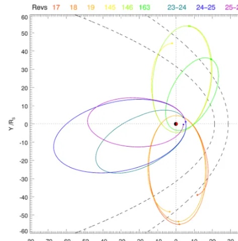
Figure 1.Plot of Cassini orbits whose data are employed in this study, colour-coded as shown at the top of the figure, corresponding to the inbound and outbound passes of Revs 17–19, 145, 146, and 163, together with the apoapsis passes from the outbound pass of Rev 23 to the inbound pass of Rev 26. These orbits are all near-equatorial and are shown looking down on Saturn’sx–yequatorial plane from the north, where the associatedzaxis is aligned with the planet’s spin (and magnetic) axis, thex–z plane contains the Sun, andypoints towards dusk (KSMAG coordinates). The dashed lines show the magnetopause and bow shock for a typical solar wind dynamic pressure of∼0.03 nPa, according to the models of Kanani et al. (2010) and Masters et al. (2008), respectively.
For definiteness, the start and end times of these passes, cor-responding to apoapsis and periapsis, respectively, or vice versa, are given as year and decimal day of year (DOY) in Ta-ble 2. For reasons discussed below we have chosen to focus on Revs lying close to the planetary equatorial plane. These orbits are shown colour-coded in Fig. 1, where we view the planet’s equatorial plane from the north. In this kronocentric solar magnetic (KSMAG) coordinate systemzpoints along the planet’s spin (and magnetic) axis positive northward, the
x–zplane contains the Sun, and (as in KSM)ypoints towards dusk (e.g., Arridge et al., 2008). A magnetopause and bow shock corresponding to a typical solar wind dynamic pres-sure of 0.03 nPa are also shown, derived from the models of Kanani et al. (2010) and Masters et al. (2008), respectively.
[image:3.612.48.284.279.490.2]of the magnetopause is then estimated from the observed position on each pass using the paraboloid surface given by Eq. (1), specifically using the last position inbound and the first position outbound in the case of multiple boundary crossings, and this value is then taken to apply to the whole of the pass. We thus assume that the magnetopause remains fixed at the value determined from the crossing throughout each pass. However, since each pass lasts typically for a few days, this assumption certainly represents a rough approx-imation. We note that although for consistency we employ the paraboloid approximation (Eq. 1) to determine the sub-solar magnetopause distances from the observed positions, the values do not differ greatly from those obtained from the more detailed Kanani et al. (2010) model shown in Fig. 1. This is explored in more detail in the Appendix, where we show that since the Kanani et al. model flares away from the subsolar position a little more strongly than for the parabola employed here, the subsolar distances determined from the latter are a little larger than those determined from the Kanani et al. model, but only by∼10–15 %. Such differences are not considered significant given the other assumptions outlined above. With the subsolar magnetopause distance for a par-ticular pass so determined, we then iterate the other model parameters, starting from the most appropriate set shown in Table 1, until an optimal fit is obtained, as discussed further in Sect. 4 below.
While the procedure described above is appropriate to the Revs which span the dawn, noon, and dusk sectors, for which the orbits intersect the magnetopause as shown in Fig. 1, it is clearly not appropriate to the nightside passes on Revs 23– 26 for which this is not the case. Instead, in these cases we compare these data with a set of models representative of compressed, intermediate, and expanded conditions, specifi-cally using updated model parameters determined in Sect. 5 from fitting to the data derived from Revs 17–19, 145, 146, and 163. These results will be presented in Sect. 6.
4 Fits for Revs 17–19 and 145, 146, and 163
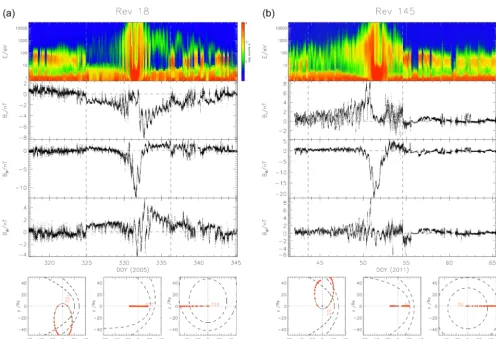
In Fig. 2 we show data for two representative Revs em-ployed in this study, specifically for Rev 18 centred in the dawn sector (Fig. 2a) and 145 centred in the dusk sector (Fig. 2b). From top to bottom the panels of these figures show (i) an electron count rate spectrogram obtained by the Cassini Plasma Spectrometer-Electron Spectrometer (CAPS-ELS) instrument covering the energy range ∼0.6–28 keV employed to help plasma regime identification, (ii) the three components of the magnetic field in spherical polar coordi-nates referenced to the planet’s spin (and magnetic) axis from which the Burton et al. (2010) model of the internal plan-etary field has been subtracted (the “residual” field), radial component Br, co-latitudinal componentBθ, and azimuthal componentBφ, and (iii) the spacecraft trajectory in KSMAG coordinates mapped to thex–y,x–z, andy–zplanes together
with the Kanani et al. (2010) magnetopause and Masters et al. (2008) bow shock models for 0.03 nPa as in Fig. 1. Time along the bottom of the upper panels is given in DOY for the year in question, 2005 for Rev 18 in Fig. 2a and 2011 for Rev 145 in Fig. 2b, and beginning of day markers are shown by circles on the trajectory plots at the bottom of the figure. The vertical dashed lines in the upper panels show the last mag-netopause crossing inbound, and the first crossing outbound, from which the radial distance of the subsolar magnetopause
R1has been estimated for each pass as discussed in Sect. 3. Of the three spherical polar components of the residual field shown in Fig. 2, here we choose to focus on modelling the co-latitudinal componentBθ which is orthogonal to the equatorial plane of the spacecraft orbit, positive southward. This component, taken together with the co-latitudinal plan-etary field, specifically describes the distribution of magnetic flux passing through the planetary equatorial plane. As previ-ously demonstrated, e.g., by Vogt et al. (2011) in the case of Jupiter’s magnetosphere, a reliable mapping from the equa-tor to the ionosphere, where the field is dominated by the planetary field, is then assured by conservation of magnetic flux, irrespective of the exact behaviour of the field lines in between. The latter behaviour depends, for example, on the detailed position and width of the equatorial ring current sheet, which strongly influences the observed equatorial val-ues of the residual radial fieldBr, as well as the azimuthal fieldBϕassociated with plasma sub-corotation sweepback of the field lines (whose associated field-aligned current is not included in the present model as indicated in Sect. 2). How-ever, this will not similarly affect theBθ component near-normal to the equatorial current sheet, whose value will be approximately unvarying through the sheet structure as guar-anteed by Gauss’s law for the magnetic field (divB=0). For these reasons, modelling studies of the near-equatorial residualBrandBϕ field components optimally require data from inclined spacecraft orbits that cut north-south through the current sheet (e.g., Kellett et al., 2009), rather than the equatorial orbits selected here for optimal modelling of the equatorialBθ component germane to the mapping problem.
Figure 2. (a)Plot showing thermal electron, magnetic field, and trajectory data for Cassini Rev 18. From top to bottom the panels show (i) a CAPS-ELS electron count rate spectrogram covering the energy range∼0.6–28 keV colour coded as shown on the right (the intense fluxes at few eV energies are principally spacecraft photoelectrons while the fluxes seen over the whole energy band closest to periapsis are due to penetrating radiation belt particles), (ii) the spherical polar radialr, co-latitudinalθ, and azimuthalϕcomponents of the magnetic field referenced to the planet’s northern spin (and magnetic) axis, from which the three-term Burton et al. (2010) model of the internal planetary field has been subtracted (except for theϕcomponent since the planetary field has no measurable azimuthal field), and (iii) the spacecraft trajectory in KSMAG coordinates mapped to thex–y,x–z, andy–zplanes together with beginning of day markers (red circles) and the Kanani et al. (2010) and Masters et al. (2008) magnetopause and bow shock models for 0.03 nPa as in Fig. 1. Time along the bottom of the upper panels is in DOY 2005. The vertical dashed lines show the last magnetopause crossing observed inbound, and the first crossing observed outbound.(b)Plot showing thermal electron, magnetic field, and trajectory data for Cassini Rev 145, in the same format as(a). In this case time along the bottom of the upper panels is in DOY 2011.
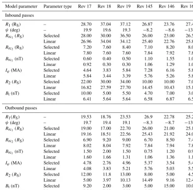
in passing that Table 3 also shows parameter values for each pass determined from linear fits to the overall parameter data, the “linear” values in the table, which will be derived and dis-cussed in Sect. 5. For the “selected” parameters, however, it can be seen, for example, that for Rev 18 shown in Fig. 2a the magnetosphere was significantly expanded on the inbound pass,R1≈37RS, but relatively compressed on the outbound pass,R1≈19RS, with an outer ring current radius and field strength that respond accordingly, while the inner ring cur-rent radius is relatively unchanged. On the other hand, for Rev 145 the subsolar magnetopause was almost unchanged in position on the two passes, at R1≈27RS intermediate between the two values for Rev 18. The fitted ring current parameters were also determined to be similar on the two
passes, again intermediate between those obtained for Rev 18 inbound and outbound.
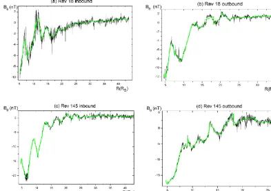
[image:5.612.49.545.61.399.2]Figure 3.Plots showing the residual co-latitudinal fieldBθversus radial distanceR(RS)together with paraboloid model results for(a)Rev 18 inbound,(b) Rev 18 outbound,(c)Rev 145 inbound, and(d)Rev 145 outbound. The data in each panel are shown in black, while coloured lines show model profiles for the “selected” parameters on each pass as given in Table 3, namely the field due to the ring current (light blue), the tail current (magenta), and the magnetopause current (dark blue), together with the total residual field given by the sum of these components (green). The red line similarly shows the total residual field corresponding to the linear approximation parameters appropriate to the estimated subsolar magnetopause radial distances for each pass (Eq. 4), also given in Table 3. The black vertical dotted line shows the magnetopause limit of applicability of the model.
from the “linear approximation” parameter set that combines together the “selected” results in Table 3 into a single model parameterised by the subsolar magnetopause distanceR1, as will be discussed in Sect. 5.
To quantitatively assess the uncertainties in the fit, we first define a “smooth fitted” field profile {Bθ} that eliminates small-scale fluctuations in the residual field which the model does not aim to reproduce. The observed field is divided into three intervals depending on radial distance. In the first in-terval, within 15RSof the planet, the residual field increases rapidly with radial distance from negative values closer to the planet, and is approximated by parabolic fits to the field taken 200 data points (1 min resolution) at a time. In the second in-terval, between 15 and 25RS, the field increases less quickly with distance, and is approximated by linear fits taken 400 data points at a time. In the third interval, at distances within the magnetopause exceeding 25RS, the field has little over-all trend, and is approximated by constant terms taken 800 data points at a time. The fits are determined by the ordinary least squares procedure. Examples are presented in Fig. 4a–d, where the black lines show the original data for the inbound and outbound passes of Revs 18 and 145 as in Fig. 3, while the green lines show the smooth fitted profiles for each pass determined using the above procedure.
The magnitude of the differences between the “selected” (and “linear”) model fits and the data have then been deter-mined using these smooth fitted profiles. The absolute error
1and the relative errorδ between the modelBθM and the smooth fitted field{Bθ}in any interval of data are taken to be given by
1= hBθM− {Bθ}i, (3a)
and
δ= 1
h|{Bθ}|i +3σ
, (3b)
Table 3.Selected and linear model parameters for the inbound and outbound passes of Revs 17–19, 145, 146, and 163.
Model parameter Parameter type Rev 17 Rev 18 Rev 19 Rev 145 Rev 146 Rev 163
Inbound passes
R1(RS) – 28.70 37.04 37.12 26.87 23.76 27.43
ψ(deg) – 19.9 19.6 19.3 −8.2 −8.6 −13.7
Rrc1 (RS) Selected 28.00 30.00 36.50 26.00 23.00 26.50
Linear 26.96 34.04 34.12 25.40 22.76 25.88
Rrc2 (RS) Selected 7.20 7.60 8.40 7.10 8.20 8.00
Linear 7.80 7.60 7.60 7.84 7.92 7.83
Brc1(nT) Selected 0.60 0.40 0.50 1.10 1.55 1.00
Linear 0.92 0.30 0.30 1.06 1.29 1.02
Iϕ(MA) Selected 4.64 3.83 5.84 7.28 6.16 5.82
Linear 5.84 3.44 3.39 5.76 5.26 5.80
R2(RS) Selected 22.00 30.00 34.00 10.00 10.00 7.00
Linear 16.82 27.59 27.70 14.45 10.43 15.17
Bt(nT) Selected 10.00 5.00 5.50 4.70 7.00 3.00
Linear 6.41 5.64 5.64 6.58 6.87 6.53
Outbound passes
R1(RS) – 19.53 18.76 23.53 26.9 22.78 25.29
ψ(deg) – 19.7 19.4 19.1 −8.3 −8.7 −13.8
Rrc1 (RS) Selected 19.00 17.00 22.70 26.00 21.00 25.10
Linear 19.16 18.51 22.56 25.43 21.92 24.06
Rrc2 (RS) Selected 6.90 9.20 9.00 6.70 8.50 7.40
Linear 8.02 8.04 7.92 7.84 7.94 7.88
Brc1(nT) Selected 1.50 2.00 1.50 0.75 1.20 0.95
Linear 1.60 1.66 1.31 1.06 1.36 1.18
Iϕ(MA) Selected 4.78 2.76 4.96 5.37 3.54 5.46
Linear 4.08 3.83 5.21 5.76 5.03 5.55
R2(RS) Selected 12.00 11.8 13.00 8.00 5.00 4.50
Linear 5.00 3.97 10.13 14.49 9.16 12.41
Bt(nT) Selected 9.20 2.00 3.00 5.00 15.00 10.00
Linear 7.26 7.33 6.89 6.58 6.95 6.72
this study, specifically for radial distances < 10, 10–17, 17– 25, and > 25RS, chosen after consideration of the behaviour of the modelled field with radial distance from the planet. The percentage errors in each region are seen to be typi-cally ∼30 %. The table also shows the errors for the mod-ified model parameters (“linear approximation”) derived in Sect. 5 below by combining the results from the individual passes.
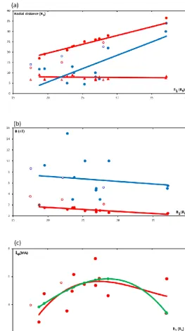
5 Linear approximation paraboloid model parameters We now combine the model parameter values determined from each of the passes for Revs 17–19, 145, 146, and 163, as given by the “selected” values in Table 3, to form an overall parameter set that depends linearly on the radial distance of the subsolar magnetopauseR1. Figure 5a shows the fit values for the radial distance parameters plotted versus R1, where the red circles and triangles show ring current outer and in-ner radius parametersRrc1 andRrc2, respectively, while the
blue circles show tail current parameterR2. The upper and lower red lines then show linear least squares fits to theRrc1
andRrc2data, respectively, while the blue line shows a linear
least squares fit toR2. The formulae for these lines are
Rrc1 =0.85R1+2.57, (4a)
Rrc2 = −0.02R1+8.49, (4b)
R2 =1.29R1−20.27, (4c)
where all distances are in units ofRS. Similarly in Fig. 5b we show the fit values for the model field strength parameters, where the red circles show the ring current field parameter
Brc1 and the blue circles the tail field parameterBt. The red
and blue lines then show the linear least squares fits given by
Brc1 = −0.07R1+3.05, (4d)
Bt = −0.09R1+9.05, (4e)
Figure 4.Illustration using data from the inbound and outbound passes of Revs 18 and 145 of the calculation of the “smooth fitted” field profiles described in Sect. 4, used to evaluate the errors between the field profiles and the “selected” parameter and “linear approximation” model field profiles. The black lines show the observed field values as in Fig. 3, while the green lines show the smooth fitted profiles.
and b also show the parameters corresponding to the initial set given in Table 1, whose values have not been included in the fits. It is seen that the tail field strengths are compara-ble, though the inner edge of the tail current is at somewhat smaller distances in the present study, while ring current ra-dial distances are also comparable, though the ring current field is somewhat weaker in the present study.
Returning to Fig. 3, the red lines in each panel show the
Bθ profiles obtained using the linear fit parameters given by Eq. (4) appropriate to the inferred values ofR1on each pass, as shown by the “linear” values in Table 3. It can be seen that these are generally similar to the individually fitted pro-files (green lines in each panel), and that they similarly fit the data reasonably well. The mean values of the absolute and relative errors of these profiles are given by the “linear approximation” values in Table 4, and can be seen to be typ-ically ∼30–50 %, of the same order as for the individually selected fit parameters.
In Fig. 5c the red circles similarly show the total ring cur-rent valuesIφ given by Eq. (2) using the selected fit param-eters (given in Table 3) plotted versus R1, to which a third order polynomial has been fitted, given by
Iφ=0.001R13−0.114R 2
1+3.724R1−33.895, (5a)
Table 4.Mean values of the absolute|1|and relative|δ|fit errors for the inbound and outbound passes of Revs 17–19, 145, 146, and 163 in four radial ranges, for both selected and linear approximation parameters.
Radial range Selected Linear
(RS) parameters approximations
|δ|(%) |1|(nT) |δ|(%) |1|(nT)
< 10 33.3 4.9 27.8 4.6
10–17 31.3 1.7 42.4 1.74
17–25 27.8 0.7 53 1.3
> 25 31.3 0.6 51 1.0
which has a maximum value of∼5.7 MA at∼27.5RS. In this expression,R1is in units ofRSandIφin MA. The open red circles showing the values from Table 1 are of compara-ble magnitude for the compressed and intermediate cases as shown, while the value for the expanded model goes off-scale at∼14 MA and is omitted from the plot. The green circles similarly show the total ring current determined from the lin-ear approximation fit parameters (also given in Table 3), for which the corresponding fit is
Iφ= −0.0007R31+0.0362R 2
[image:8.612.317.536.469.565.2]which exhibits only minor changes with respect to Eq. (5a) based on the selected fit parameters, and similarly has a max-imum of∼5.8 MA at∼28.7RS.
Comparing the results in Fig. 5 with those of the earlier ring current study by Bunce et al. (2007), who employed data from the first 2 years of Cassini data together with Pioneer11 and Voyager data, it can be seen that the overall trends are similar. Over the same radial range of subsolar magnetopause distances as investigated by these authors, ∼17–27RS, we find a similar increase in the radial distance of the outer edge of the current sheet, a similar unresponsiveness in the ra-dial distance of inner edge of the current sheet located near ∼7RS, and a similar increase in the total current, though only between∼3 and ∼6 MA in our case, compared with ∼9 to∼15 MA as determined by Bunce et al. (2007). Be-yond these radial distances in the present study, however, the total ring current is then found to fall to smaller values again at subsolar magnetopause distances up to∼37RS.
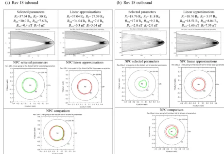
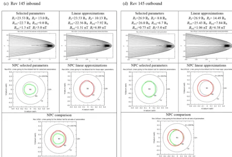
To be sure our fitted models provide a reasonable result not only along the specific Cassini trajectories employed in the study but also throughout Saturn’s magnetosphere, we have calculated model field lines between the ionosphere and 200RS down Saturn’s tail. Results are shown for our rep-resentative Revs in Fig. 6, where Fig. 6a and b show the models for Rev 18 inbound and outbound, respectively, while Fig. 6c and d similarly show the models for Rev 145 inbound and outbound, respectively. In these figures the upper pan-els show field lines traced in thex–zplane (noon-midnight meridian) in KSM coordinates, for the selected parameters on the left and for the linear approximations on the right (Ta-ble 3). The IMF in these calculations was assumed equal to zero, so that the field lines in the more distant tail beyond typically ∼100RS become near-parallel to thex axis with essentially no closed flux crossing the equator at these dis-tances and beyond, such that the “open” magnetic flux in the tail lobes becomes near-constant. It is then of interest to calculate the region in the polar ionosphere to which this tail lobe flux maps, and to consider its relation to the ob-served location of the open-closed field boundary in Saturn’s magnetosphere and to the auroral oval. The middle panels of Fig. 6 thus show the northern ionospheric projections of the field lines that reach x= −200RS, this distance lying well within the regime of near-constant tail lobe flux in all cases. Again, results for the selected parameters are shown on the left (green line) and for the linear approximations on the right (red line), which are then compared in the lower panel of Fig. 6. It can be seen that these regions are generally, but not always, similar to each other.
It can further be seen from the results in Fig. 6 that in most cases the ionospheric region mapping into the model tail extends to∼10◦from the northern pole, but with an off-set towards the nightside, so that it is located a degree or two poleward of this co-latitude on the dayside, and a degree or two equatorward of this co-latitude on the nightside. We then note that Jinks et al. (2014) found that the open-closed
boundary lies on average at∼13.3◦in the Northern Hemi-sphere (as shown in Fig. 6), in a multi-instrument study of Cassini data in the dusk to midnight sector, compatible with these results. They also found that the poleward boundary of the main upward field-aligned current region, presumed as-sociated with the main auroral region, lay on average∼1.8◦ equatorward of this in the Northern Hemisphere, thus typi-cally at∼15.1◦in this LT sector, compatible with the results of Hunt et al. (2015). Given a similar small equatorward dis-placement of the auroral oval from the open-closed bound-ary in the near-noon sector, we would thus expect its pole-ward boundary in the Northern Hemisphere to lie just equa-torward∼10◦on the basis of most of the results in Fig. 6. This expectation is then compatible with the study of north-ern dayside UV auroral emissions observed in Hubble Space Telescope data by Belenkaya et al. (2014), where the pole-ward boundary (in “non-storm” cases) was found typically to be near∼11◦co-latitude, similar to the poleward half-power points found in this LT sector by Carbary (2012) from a sta-tistical study of Cassini UV emission data. Overall, we thus conclude that the tail magnetic flux in our models generally provides a good representation of the open tail flux in Sat-urn’s magnetosphere, closely related to the size of SatSat-urn’s auroral ovals.
6 Application of linear approximation model parameters to nightside data
In this section we now test the ability of the model to account for magnetic field observations on the nightside of Saturn. To do this we employ data from Revs whose apoapsides lay in the tail, and consider full apoapsis passes from the outbound pass of one Rev to the inbound pass of the next, recalling that Cassini Revs are defined from apoapsis to apoapsis. Specif-ically we employ data from three apoapsis passes, from the outbound pass of Rev 23 to the inbound pass of Rev 26. As discussed in Sect. 3, since the spacecraft did not cross the magnetopause during these Revs we have no means to esti-mate the radial distance of the subsolar magnetopauseR1. In-stead we compare these data with three representative models corresponding to compressed, intermediate, and expanded conditions with subsolar magnetopause distances of 17.5, 22, and 28RS, respectively, as in Belenkaya et al. (2008), but now using the updated linear approximation parameters given by Eqs. (4a)–(4e). For definiteness these parameters are given in Table 5. We note that we have also examined these data in relation to the original parameter sets for these
R1values given in Table 1, but find that these generally give less satisfactory results due mainly to over-estimates of the strength of the ring current field (see Fig. 5b).
Figure 5.“Selected” model parameters for each pass as given in Table 3 are shown plotted versus the estimated distance to the subsolar magnetopauseR1(RS)on each pass, together with least-squares fitted lines. Panel(a)shows the radial distance parameters of the model, where the filled red circles and triangles show the outer and inner boundaries of the ring currentRrc1 andRrc2, respectively, while the filled
blue circles show the radial distance of the inner edge of the tail currentR2. The red and blue lines then show linear least squares fits to these data, given by Eqs. (4a)–(4c). The corresponding open symbols show the parameters corresponding to the models proposed by Belenkaya et al. (2008) given in Table 1, which are not included in the fits. Panel(b)similarly shows the model field parameters, where the filled red circles show the ring current field strengthBrc1and the filled blue circles the tail field parameterBt. Least squares linear fits are shown by the
Figure 6.
Table 5.Linear approximation model parameters for compressed, intermediate, and expanded states, corresponding to subsolar mag-netopause distances of 17.5, 22, and 28RS, respectively.
Linear Compressed Intermediate Expanded approximation
parameters
R1(RS) 17.5 22.0 28.0
Rrc1 (RS) 17.44 21.26 26.36
Rrc2 (RS) 8.07 7.96 7.81
Brc1(nT) 1.75 1.42 0.97
R2(RS) 2.34 8.16 15.91
Bt(nT) −7.44 −7.03 −6.48
this orbit (Fig. 1), here we concentrate on the magnetic data within 50RS. Model results are shown in these figures by the red, green, and blue lines for the compressed, intermedi-ate, and expanded linear approximation models, respectively, given in Table 5. It can be seen that the models for intermedi-ate and expanded stintermedi-ates are in reasonable accord with the data for both passes shown. This is quantified in Table 6 where we give the mean values of the moduli of the absolute|1|and relative |δ|errors given by Eqs. (3a) and (3b), respectively,
in four radial ranges for each of the three apoapsis passes in-vestigated, in a similar manner to Table 4. Overall it can be seen that the errors for the intermediate and expanded mod-els are generally comparable, and smaller than those for the compressed model.
7 Discussion and conclusions
[image:11.612.53.280.469.580.2]sub-Figure 6. (a)and(b)show results of model field line calculations between the ionosphere and 200RS down tail for(a)Rev 18 inbound and (b) Rev 18 outbound, as illustrated in Figs. 2–4. The upper panels show field lines traced in the noon-midnight meridian plane in KSM coordinates, for the selected model parameters for these passes on the left and the linear approximations on the right, as given by the parameters above the field line plots. The IMF was assumed equal to zero. The middle panels show the northern ionospheric projections of the field lines that reachx= −200RSviewed looking down on the north pole again for the selected parameters on the left (green line) and the linear approximations on the right (red line). These are compared in the lower panel.(c)and(d)show results of model field line calculations between the ionosphere and 200RSdown tail for(c)Rev 145 inbound and(d)Rev 145 outbound, in the same format as(a) and(b).
Table 6.Mean values of the absolute|1|and relative|δ|fit errors for the apoapsis passes from Rev 23 outbound to 26 inbound in four radial ranges, for three assumed states of the magnetosphere, compressed, intermediate, and expanded, using the linear approximation model parameters in Table 5.
Radial range Compressed Intermediate Expanded (RS)
|δ|(%) |1|(nT) |δ|(%) |1|(nT) |δ|(%) |1|(nT)
< 10 42.2 5.8 29.3 3.9 24.5 3.1
10–17 69.5 3.3 42.5 1.6 41.2 1.8
17–25 103.2 2.0 78.8 1.5 66.9 1.5
> 25 39.3 0.3 27.5 0.3 23.0 0.3
solar radial distance of the magnetopause, governed physi-cally by pressure balance at the boundary depending on the dynamic pressure of the upstream solar wind, is taken to set the basic spatial scale of the system, on which the other pa-rameters may depend. A small penetrating component of the
IMF may also be added, but for simplicity has not been em-ployed in the present study.
[image:12.612.149.448.534.628.2]Figure 7.Plots showing the residual co-latitudinal fieldBθ versus radial distanceR (RS)together with paraboloid model results for (a)Rev 24 outbound, and(b)Rev 25 inbound. Model results are shown by the red, green, and blue lines for the compressed, inter-mediate, and expanded linear approximation models, respectively, whose parameters are given in Table 5.
both inbound and outbound passes. The position of the sub-solar boundary was then estimated and applied to the data from each pass individually. These 12 passes span LTs from pre-dawn via noon to post-dusk. We focus on modelling the co-latitudinal field component that defines the magnetic flux passing through the equatorial plane, and determine the pa-rameters that best fit the data on each pass. Overall errors for the residual field, with planetary field subtracted, are typi-cally∼30 %. The best-fit parameters from each pass are then used to determine linear dependencies of the parameters on the subsolar radial distance to the magnetopause, thus pro-viding formulae for these parameters for any value of the ra-dial distance. The variation of the ring current parameters is found to show similar behaviour to that determined previ-ously by Bunce et al. (2007). However, the parameters of the tail current system show significant fluctuations about the fit-ted lines, and differences from values determined in previous studies, perhaps indicative of the occurrence of internal dy-namics unconnected with the scale size of the system set by the solar wind. Overall, the fits to the residual field obtained
using these linear approximation parameters are found to be comparably good relative to those determined from the indi-vidually selected parameters. In addition, the “open” flux in the tail lobes in these models is found usually to be in reason-able accord, when mapped to the ionosphere, with the empir-ically determined location of the open-closed field boundary in the ionosphere, as well as with the location of the auroral oval whose poleward boundary is typically located a degree or two equatorward (Carbary, 2012; Jinks et al., 2014; Be-lenkaya et al., 2014; Hunt et al., 2015).
We then investigated the field data on six passes through the magnetospheric tail, for which the spacecraft did not cross the magnetopause. In these cases we compared the observations with three linear approximation models repre-sentative of compressed, intermediate, and expanded states. Reasonable agreement was found in these cases with models representing intermediate or expanded states.
8 Data availability
Appendix A: Comparison of subsolar magnetopause distances estimated from observed boundary crossings using the paraboloid and Kanani et al. (2010) models In the analysis undertaken in this paper we are required to es-timate the radial distance of the subsolar magnetopause from a local observation of the boundary at some general point (xmp,ymp,zmp)in KSM coordinates. The values employed here are straightforwardly determined from solution of the quadratic in R1formed by Eq. (1). Here we compare these values with those estimated from the more detailed empiri-cal model derived by Kanani et al. (2010). In this model the magnetopause surface is taken to be given by
R=R0
2
1+cosθ
K
, (A1)
whereRis radial distance from the planet,θis the co-latitude angle from the KSMx axis (directed towards the Sun), and
R0is the subsolar magnetopause distance. The latter parame-ter together with exponentKare defined in terms of the solar wind dynamic pressureDP(in nPa) as
R0=a1D−Pa2, (A2)
and
K=a3+a4DP, (A3)
where the empirically determined coefficients are a1= 10.3RS,a2=0.2,a3=0.73, anda4=0.4.
We thus note that the ratio between the magnetopause distance at the subsolar point and, e.g., on the dawn-dusk meridian is 2K≈1.66 in the Kanani et al. (2010) model (for moderate pressures), compared with 21/2≈1.41 for the paraboloid model given by Eq. (1). The Kanani et al. model magnetopause thus flares away from the subsolar point to a somewhat greater degree than the paraboloid model. Conse-quently, given a boundary observation at some general point (xmp, ymp, zmp), or equivalently at some radial distance R and co-latitude angleθwith respect to thexaxis, the estimate of the subsolar distance to the boundary using the paraboloid model will be slightly larger than for the Kanani et al. (2010). Substituting forDPfrom Eq. (A2) into Eq. (A3), and hence into Eq. (A1), the estimate from the Kanani et al. (2010) model is obtained by iterative solution forR0of
R=R0
2
1+cosθ
a3+a4(a1/R0)1/a2
. (A4)
Competing interests
The authors declare that they have no conflict of interest.
Acknowledgements. Work at the Federal State Budget Educa-tional Institution of Higher Education M. V. Lomonosov Moscow State University, Skobeltsyn Institute of Nuclear Physics (SINP MSU) was partially supported by the RFBR grant 16-05-00760. Work at Leicester was supported by STFC consolidated grants ST/K001000/1 and ST/N000749/1. We thank I. I. Alexeev for ac-cess to his paraboloid model codes.
The topical editor, E. Roussos, thanks J. Carbary and one anony-mous referee for help in evaluating this paper.
References
Achilleos, N., Guio, P., and Arridge, C. S.: A model of force balance in Saturn’s magnetodisc, Mon. Not. R. Astron. Soc., 401, 2349– 2371, doi:10.1111/j.1365-2966.2009.15865.x, 2010.
Alexeev, I. I., Kalegaev, V. V., Belenkaya, E. S., Bobrovnikov, S. Y., Bunce, E. J., Cowley, S. W. H., and Nichols, J. D.: A global magnetic model of Saturn’s magnetosphere, and a com-parison with Cassini SOI data, Geophys. Res. Lett., 33, L08101, doi:10.1029/2006GL025896, 2006.
Arridge, C. S., Khurana, K. K., Russell, C. T., Southwood, D. J., Achilleos, N., Dougherty, M. K., Coates, A. J., and Leinweber, H. K.: Warping of Saturn’s magnetospheric and magnetotail current sheets, J. Geophys. Res., 113, A08217, doi:10.1029/2007JA012963, 2008.
Belenkaya, E. S., Cowley, S. W. H., and Alexeev, I. I.: Saturn’s au-rora in the January 2004 events, Ann. Geophys., 24, 1649–1663, doi:10.5194/angeo-24-1649-2006, 2006a.
Belenkaya, E. S., Alexeev, I. I., Kalegaev, V. V., and Blokhina, M. S.: Definition of Saturn’s magnetospheric model parame-ters for the Pioneer 11 flyby, Ann. Geophys., 24, 1145–1156, doi:10.5194/angeo-24-1145-2006, 2006b.
Belenkaya, E. S., Alexeev, I. I., Blokhina, M. S., Cowley, S. W. H., Badman, S. V., Kalegaev, V. V., and Grigoryan, M. S.: IMF dependence of the open-closed field line boundary in Saturn’s ionosphere, and its relation to the UV auroral oval observed by the Hubble Space Telescope, Ann. Geophys., 25, 1215–1226, doi:10.5194/angeo-25-1215-2007, 2007.
Belenkaya, E. S., Cowley, S. W. H., Badman, S. V., Blokhina, M. S., and Kalegaev, V. V.: Dependence of the open-closed field line boundary in Saturn’s ionosphere on both the IMF and solar wind dynamic pressure: comparison with the UV auro-ral oval observed by the HST, Ann. Geophys., 26, 159–166, doi:10.5194/angeo-26-159-2008, 2008.
Belenkaya, E. S., Alexeev, I. I., Blokhina, M. S., Bunce, E. J., Cowley, S. W. H., Nichols, J. D., Kalegaev, V. V., Petrov, V. G., and Provan, G.: IMF dependence of Saturn’s auroras: mod-elling study of HST and Cassini data from 12–15 February 2008, Ann. Geophys., 28, 1559–1570, doi:10.5194/angeo-28-1559-2010, 2010.
Belenkaya, E. S., Cowley, S. W. H., Nichols, J. D., Blokhina, M. S., and Kalegaev, V. V.: Magnetospheric mapping of the dayside UV auroral oval at Saturn using simultaneous HST images, Cassini
IMF data, and a global magnetic field model, Ann. Geophys., 29, 1233–1246, doi:10.5194/angeo-29-1233-2011, 2011.
Belenkaya, E. S., Cowley, S. W. H., Kalegaev, V. V., Barinov, O. G., and Barinova, W. O.: Magnetic interconnection of Saturn’s po-lar regions: comparison of modelling results with Hubble Space Telescope UV auroral images, Ann. Geophys., 31, 1447–1458, doi:10.5194/angeo-31-1447-2013, 2013.
Belenkaya, E. S., Cowley, S. W. H., Meredith, C. J., Nichols, J. D., Kalegaev, V. V., Alexeev, I. I., Barinov, O. G., Barinova, W. O., and Blokhina, M. S.: Magnetospheric magnetic field modelling for the 2011 and 2012 HST Saturn aurora campaigns – impli-cations for auroral source regions, Ann. Geophys., 32, 689–704, doi:10.5194/angeo-32-689-2014, 2014.
Bunce, E. J., Cowley, S. W. H., Alexeev, I. I., Arridge, C. S., Dougherty, M. K., Nichols, J. D., and Russell, C. T.: Cassini observations of the variation of Saturn’s ring current parameters with system size, J. Geophys. Res., 112, A10202, doi:10.1029/2007JA012275, 2007.
Bunce, E. J., Arridge, C. S., Cowley, S. W. H., and Dougherty, M. K.: Magnetic field structure of Saturn’s dayside magne-tosphere and its mapping to the ionosphere: Results from ring-current modelling, J. Geophys. Res., 113, A02207, doi:10.1029/2007JA012538, 2008.
Burton, M. E., Dougherty, M. K., and Russell, C. T.: Saturn’s in-ternal planetary magnetic field, Geophys. Res. Lett., 37, L24105, doi:10.1029/2010GL045148, 2010.
Carbary, J. F.: The morphology of Saturn’s ultraviolet aurora, J. Geophys. Res., 117, A06210, doi:10.1029/2012JA017670, 2012. Hunt, G. J, Cowley, S. W. H., Provan, G., Bunce, E. J., Alex-eev, I. I., Belenkaya, E. S., Kalegaev, V. V., Dougherty, M. K., and Coates, A. J.: Field-aligned currents in Saturn’s south-ern nightside magnetosphere: Sub-corotation and planetary pe-riod oscillation components, J. Geophys. Res., 119, 9847–9899, doi:10.1002/2014JA020506, 2014.
Hunt, G. J, Cowley, S. W. H., Provan, G., Bunce, E. J., Alexeev, I. I., Belenkaya, E. S., Kalegaev, V. V., Dougherty, M. K., and Coates, A. J.: Field-aligned currents in Saturn’s northern night-side magnetosphere: Evidence for inter-hemispheric current flow associated with planetary period oscillations, J. Geophys. Res., 120, 7552–7584, doi:10.1002/2015JA021454, 2015.
Jinks, S. L., Bunce, E. J., Cowley, S. W. H., Provan, G., Yeo-man, T. K., Arridge, C. S., Dougherty, M. K., Gurnett, D. A., Krupp, N., Kurth, W. S., Mitchell, D. G., Morooka, M., and Wahlund, J. E.: Cassini multi-instrument assessment of Sat-urn’s polar cap boundary, J. Geophys. Res., 119, 8161–8177, doi:10.1002/2014JA020367, 2014.
Kanani, S. J., Arridge, C. S., Jones, G. H., Fazakerley, A. N., McAn-drews, H. J., Sergis, N., Krimigis, S. M., Dougherty, M. K., Coates, A. J., Young, D. T., Hansen, K. C., and Krupp, N.: A new form of Saturn’s magnetopause using a dynamic pressure balance model, based on in situ, multi-instrument Cassini measurements, J. Geophys. Res., 115, A06207, doi:10.1029/2009JA014262, 2010.
Kellett, S., Bunce, E. J., Coates, A. J., and Cowley, S. W. H.: Thickness of Saturn’s ring current determined from north-south Cassini passes through the current layer, J. Geophys. Res., 114, A04209, doi:10.1029/2008JA013942, 2009.
observations, Eos Trans. AGU, 87, Jt. Assem. Suppl., Abstract P44A-01, 2006.
Masters, A., Achilleos, N., Dougherty, M. K., Slavin, J. A., Hospo-darsky, G. B., Arridge, C. S., and Coates, A. J.: An empir-ical model of Saturn’s bow shock: Cassini observations of shock location and shape, J. Geophys. Res., 113, A10210, doi:10.1029/2008JA013276, 2008.