Wave transformation models with exact second-order transfer
H. Bredmose
a,∗, Y. Agnon
b, P.A. Madsen
c, H.A. Schäffer
a aDHI Water & Environment, Agern Allé 5, DK-2970 Hørsholm, DenmarkbDepartment of Civil and Environmental Engineering, Technion, Haifa 32000, Israel
cDepartment of Mechanical Engineering, Technical University of Denmark, Building 403, DK-2800 Kgs. Lyngby, Denmark
Received 10 March 2004; received in revised form 24 November 2004; accepted 6 December 2004 Available online 24 June 2005
Abstract
Fully dispersive deterministic evolution equations for irregular water waves are derived. The equations are formulated in the complex amplitudes of an irregular, directional wave spectrum and are valid for waves propagating in directions up to
±90◦from the main direction of propagation under the assumptions of weak nonlinearity, slowly varying depth and negligible reflected waves. A weak deviation from straight and parallel bottom contours is allowed for. No assumptions on the vertical structure of the velocity field is made and as a result, the equations possess exact second-order bichromatic transfer functions when comparing to the reference solution of a Stokes-type analysis. Introduction of the so-called ‘resonance assumption’ leads to the evolution equations of among others Agnon, Sheremet, Gonsalves and Stiassnie [Coastal Engrg. 20 (1993) 29–58]. For unidirectional waves, the bichromatic transfer functions of the ‘resonant’ models are found to have only small deviations in general from the reference solution. We demonstrate that the ‘resonant’ models can be solved efficiently using Fast Fourier Transforms, while this is not possible for the ‘exact’ models. Simulation results for unidirectional wave propagation over a submerged bar show that the new models provide a good improvement from linear theory with respect to wave shape. This is due to the quadratic terms, enabling a nonlinear description of shoaling and de-shoaling, including the release of higher harmonics after the bar. For these simulations, the similarity between the ‘exact’ and ‘resonant’ models is confirmed. A test case of shorter waves, however, shows that the amplitude dispersion can be quite over-predicted in the models. This behaviour is investigated and confirmed through a third-order Stokes-type perturbation analysis.
2005 Elsevier SAS. All rights reserved.
Keywords: Nonlinear wave transformation; Deterministic spectral modelling; Fully dispersive wave theory; Fast Fourier Transform; Bichromatic transfer; Amplitude dispersion
1. Introduction
When a wave field propagates over varying depth, the wave spectrum changes due to shoaling, refraction and nonlinear interactions. Numerous wave models can be used to model these effects, varying from solving the Navier–Stokes equations, allowing for a free surface, over Boussinesq modelling in the time domain, to simple linear shoaling calculations. For large wave fields of two horizontal dimensions, Navier–Stokes modelling is too computationally demanding and Boussinesq modelling still
* Corresponding author.
E-mail addresses: [email protected] (H. Bredmose), [email protected] (Y. Agnon), [email protected] (P.A. Madsen), [email protected] (H.A. Schäffer).
requires an extensive computational effort. For practical use, there is thus an interest in computationally faster models, yet being more accurate than a simple linear wave shoaling calculation.
Evolution equations for the wave amplitudes of a complex wave spectrum represent a model class of this type. In such models, time periodicity of the wave field is assumed, allowing for expanding the wave field as a Fourier series in time. The Fourier coefficients are then functions of space, and under the assumptions of (1) negligible reflected waves, (2) slowly varying depth and (3) weak nonlinearity, first-order differential equations for the spatial evolution of the Fourier amplitudes can be derived. In this approach, the wave field in a physical domain can thus be found by integrating a set of first-order ordinary differential equations in one spatial sweep, taking refraction, shoaling and nonlinear interactions into account. If the phases of the Fourier amplitudes are retained in the modelling, the evolution equations are called deterministic. We shall focus on deterministic evolution equations in this paper. The models derived provide a numerically efficient tool for the description of shoaling, refraction and quadratic nonlinear interactions for wave fields in two horizontal dimensions.
Evolution equations are appropriate for describing nonlinear interactions between wave components. On an even depth quadratic interactions can be removed from the equations and evolution equations describing four-wave interactions (cubic nonlinearity) can be derived (see e.g. [1]). On variable depth, however, the quadratic interactions can be resonant in the form of class III Bragg resonance [2] and can thus not be eliminated. Further, in shallow water quadratic interactions can be nearly resonant, giving so-called triad interactions [3]. Contrary to four-wave interactions at deep water, triad interactions can build up over just a few wave lengths in shallow conditions and are thus important in coastal areas. Away from shallow and intermediate water, the quadratic interactions are non-resonant, giving rise to second-order bound waves, being phase locked to the first-order wave field. In this paper we shall retain only quadratic nonlinearity, thereby precluding any description of four-wave interactions. The models derived will provide a correct description of the second-order wave field from deep to shallow water, cubic effects being discarded.
Deterministic evolution equations have often been derived using a time domain Boussinesq formulation as starting point. Examples are Freilich and Guza [4], Liu, Yoon and Kirby [5], Yoon and Liu [6], Madsen and Sørensen [7], Chen and Liu [8] and Kaihatu and Kirby [9]. Boussinesq formulations make an attractive starting point, since they provide a depth-integrated formulation of the governing equations for water wave propagation. On the other hand, as Boussinesq formulations are derived as asymptotic expansions of the governing equations from the shallow water limit, their accuracy generally decays in deeper water.
As an alternative, evolution equations can be derived directly from the irrotational, inviscid governing equations. Hereby, the linear phase speed and shoaling characteristics agree exactly with linear wave theory for all depths. Such models are therefore denoted fully dispersive evolution equations. Agnon et al. [10] and Kaihatu and Kirby [11] derived fully dispersive evolution equations for the complex Fourier amplitudes of the still water potential. Both derivations involved depth-integration of the Laplace equation. Here the vertical variation of the velocity potential must be known a priori, and in both works the vertical structure of a linear wave was assumed. As a result, the second-order bound wave field is not modelled with exact amplitudes. Eldeberky and Madsen [12] pointed out that a quadratic transformation is needed, when results of the two above models are transformed from the still water potential to free surface elevations. Using this transformation, they derived evolution equations formulated directly in the complex Fourier amplitudes of the free surface elevation.
In this paper, a new derivation of fully dispersive deterministic evolution equations is given, free of assumptions on the vertical variation of the velocity potential. We hereby, for the first time, obtain models having exact second-order properties. We present evolution equations formulated in the complex Fourier amplitudes of either the still water potential or the free surface elevation. Both formulations are derived for an angular spectrum representation of the wave field, allowing for wave propagation in directions up to±90◦from the main direction of wave propagation. A weak deviation from straight and parallel depth contours is allowed for. By invoking the so-called ‘resonance assumption’ within the nonlinear terms, the models of Agnon et al. [10], Kaihatu and Kirby [11] and Eldeberky and Madsen [12] are recovered. Thus for short, we denote these models the ‘resonant’ models.
Having derived ‘exact’ as well as ‘resonant’ models, we analyse them with respect to second-order transfer functions for bichromatic wave propagation. The transfer functions derived are compared to the exact solution of a Stokes-type analysis of the governing equations as given by Sharma and Dean [13]. As expected the transfer of the ‘exact’ models is identical to the reference solution.
to the angular spectrum variation, such that forN frequencies and M angular wave modes, the evolution equations can be solved at a cost of O((MlogM)(NlogN )). This speed-up, however, is not applicable to the ‘exact’ models.
Although the ‘exact’ and ‘resonant’ models are derived for two-dimensional wave propagation, we here focus the validation on unidirectional waves. The models are applied to two cases of weakly nonlinear wave propagation over a submerged bar, using the experimental data of Beji and Battjes [15]. For a test of long waves (kh=0.32 on the bar top), the second-order terms provide a clear improvement over results of linear theory, both with respect to wave shape and to release of higher harmonics as the waves leave the bar top. For a test of shorter waves (kh=0.68 at the bar top), the wave shape on the bar top is improved as well by the second-order terms, but accumulative phase errors are observed, indicating an over-prediction of the amplitude dispersion in the models.
To look further into this, we extend the Stokes-type analysis of the models to third order, to obtain results for the amplitude dispersion and third-order transfer for unidirectional waves.
The structure of the paper is as follows. In Section 2, a review of fully dispersive evolution equations is given while in Section 3, the new exact models are derived. The bichromatic transfer functions for the new models are presented in Section 4 and the numerical speed-up technique using FFT is dealt with in Section 5. Model results for wave propagation over a submerged bar are presented in Section 6, and the third-order analysis in Section 7.
2. Review of fully dispersive evolution equations
2.1. The evolution equations of Agnon et al. [10]
The evolution equations of Agnon et al. [10] were formulated in the complex Fourier amplitudes of the still water potential and are valid for one horizontal dimension. The main steps in the derivation were the following: The free surface boundary conditions were expanded around the still water level and combined into a single equation in the still water potential. A multiple scales expansion in space and time was introduced to separate the fast and slow variation of the wave field. The governing equations were next transformed to Fourier space (with respect to time) and the Laplace equation depth-integrated. Initially, the vertical structure of bound waves as well as free waves was considered, that is
φ(x, z, t)=coshk(z+h)
coshkh φ(x, z=0, t) (1)
wherekcan be a free wave number or a bound wave number. The model derived, however, was based on the vertical structure of a free wave. Agnon et al. [10] defined a detuning parameter
µ=(kbound−kfree)/kfree (2)
giving a measure of the deviation between bound and free wave numbers. The bound waves within the model are thus described with an error of O(µ).
The model was extended to two dimensions in Agnon and Sheremet [16], following the angular spectrum approach of Dalrymple and Kirby [17]. They also developed stochastic evolution equations based on the deterministic model, this topic, however, is not pursued in the present paper.
2.2. The evolution equations of Kaihatu and Kirby [11]
Kaihatu and Kirby [11] derived a set of evolution equations, essentially being an extension of the model of Agnon et al. [10] to weakly two-dimensional wave propagation. Their starting point was the Laplace equation, which was depth-integrated assuming a vertical structure of the velocity field corresponding to linear waves. The resulting equation was combined with the free surface conditions, giving a nonlinear mild-slope equation. Next the following expansion was utilised
φ(x, y, t)|z=0= N
p=−N
−ig
ωp
ap(x, y)ei(
¯
kpdx−ωpt ), (3)
the model was extended to allow for a spatially varying current. For one horizontal dimension and no current, the model is identical to the model of Agnon et al. [10].
2.3. The second-order transformation fromφtoη
Both of the two above models were compared to experimental results. Agnon et al. [10] simulated a laboratory test of almost unidirectional irregular waves propagating onto an open beach, and also field measurements of shoaling waves in Walker Bay, South Africa. Kaihatu and Kirby [11] simulated the test of Whalin [18] for regular wave propagation over a semicircular shoal and the test of breaking irregular waves on a plane sloping beach of Mase and Kirby [19]. For the latter purpose, the breaking model of Mase and Kirby [19] was incorporated.
In both of these works, however, the transformation between the Fourier amplitudes of the still water level and the Fourier amplitudes of the free surface elevation was linear. This is inconsistent with the second-order accuracy of the models, as pointed out by Eldeberky and Madsen [12]. Eldeberky and Madsen [12] gave a second-order transformation between these amplitudes and transformed the evolution equations of Agnon et al. [10], as well as Agnon and Sheremet [16], to sets of evolution equations formulated directly in the complex amplitudes of the free surface elevation. The correction of the transformation improves the accuracy of super-harmonic energy transfer significantly.
Kaihatu [20] discussed this correction of the deterministic model as well. The influence of the new second-order terms was examined by deriving fully nonlinear solutions to the equations in the amplitudes of the still water potential. The solutions were then transformed to free surface elevations, using either the linear transformation or the correct second-order transformation. In shallow water, essentially no difference was found, while at deep water, the effect was found to be more pronounced.
3. Derivation of the new evolution equations
In this section we present a new derivation of fully dispersive evolution equations, leading to a model with exact second-order transfer. We first derive a set of equations formulated in the complex Fourier amplitudes of the still water level potential. Subsequently, we transform these equations to the complex Fourier amplitudes of the free surface elevation.
3.1. Governing equations and scaling
We consider the motion of an inviscid irrotational fluid, as depicted in Fig. 1. A Cartesian coordinate system(x, y, z)=(x, z)
with thez-axis pointing upwards from the still water level is adopted. The surface elevation is denotedη(x, t)and the velocity potentialφ(x, z, t). The velocity field within the fluid is(u, v, w)andgis the acceleration of gravity. The depth is described by
h(x), measuring the distance from the bottom to the still water level. The governing equations are
∇2φ+φ
zz=0, −h < z < η, (4)
φz−∇φ·∇η−ηt=0, z=η, (5)
φt+gη+(∇φ)2+φz2
/2=0, z=η, (6)
φz+∇h·∇φ=0, z= −h, (7)
[image:4.544.69.386.457.660.2]stating local continuity (4), the kinematic and dynamic free surface conditions (5), (6), and impermeability of the bottom (7). ∇is the horizontal gradient operator, i.e.,∇=(∂x∂ ,∂y∂ ). We shall assume a classical Stokes scaling of the variables, that is
x= x
k0, z=z
h
0, h=hh0,
t= t
ω0
, η=a0η, φ=
ga0
ω0
φ,
where a prime denotes dimensionless variables and(k0, h0, ω0, a0)are typical measures of wave number, depth, frequency and amplitude, respectively. This gives the nonlinearity parameterε=k0a0, which will appear as a factor on the nonlinear terms, if the above variables are inserted into the governing equations. However, instead of using the dimensionless variables, we shall carry out the derivation and analysis in the dimensional variables, keeping an artificialεfactor in front of the nonlinear terms. Thus in the following,ε is to be regarded as a small ordering parameter, which should simply be omitted in any numerical evaluation of the expressions. We thus assume weak nonlinearity of the wave field. Further, we assume that the sea bed is varying slowly as function of x, i.e.,h=h(εx), and that the deviation from uniform depth in they-direction is O(ε).
3.2. Rewriting the governing equations
We follow the lines of Madsen and Schäeffer [21] and Agnon, Madsen and Schäffer [22], taking basis in an exact power series solution to the Laplace equation. The starting point is to expand the velocity potential as a power series inz:
φ(x, z, t)=
∞
n=0
znφn(x, t). (8)
It is easily seen thatφ0=φ(x,0, t)≡Φandφ1=w(x,0, t)≡W. Further, insertion of (8) into the Laplace equation yields the well-known recursion relationφn+2= −∇2φn/((n+1)(n+2))and thereby the solution
φ(x, z, t)=
∞
n=0
(−1)nz
2n∇2n
(2n)! Φ+(−1)
nz2n+1∇2n
(2n+1)!W. (9)
We identify the above series in(z∇)as the Taylor series of the functions cos(z∇)and sin(z∇)/∇, thus allowing us to write the series as
φ(x, z, t)=Cos(z∇)Φ+ 1
∇Sin(z∇)W, (10)
where the capitalised form of the trigonometric functions has been used to indicate that they denote operators. In the above equation both series operators are even functions of∇. They are thus scalar operators, just like∇2. We indicate this by using a non-bold∇in their arguments and shall be using this convention throughout.
Next, we utilise the assumption of slowly varying depth,h=h(εx), and retain only first-order derivatives of the depth variation. As shown by Mei [23] and Agnon [24], a convenient way of dealing with this is to introduce a constant reference depthh(x)=h0+δ(x)and expand the bottom boundary condition aroundh0. This proves to be advantageous, when combining the sea bed condition with the series solution (10). We shall later resubstitute the true local depthh, and we thus note that the use of a reference level is just a technicality, that does not introduce any bounds on the depth range of model application. Taylor expanding the sea bed condition around the constant reference levelh0yields
φz+δ∇2φ+1 2δ
2∇2φ
z+∇δ·(∇φ−δ∇φz)=Oδ3, δ2∇δ, z= −h0. (11) where the Laplace equation (4) has been used to rewrite doublez-differentiations to∇2operations. To lowest order, this equation states thatφz=O(δ,∇δ), allowing for writing the sea bed condition in the compact form
φz= −∇·(δ∇φ)+O
δ3, δ2∇δ, δ(∇δ)2, z= −h0. (12) The advantage of this formulation is that it is defined on a constant level z= −h0. All effects of varying depth are thus represented byδand when the series solution (10) is inserted forφ, the operators will thus have the argumenth0∇, where ∇andh0can be interchanged. This simplifies the derivation considerably, since in generalhand∇are not interchangeable. The assumption of mildly sloping bottom allows us to neglect all but first-order derivatives ofδ, while as the last step in the derivation, we can replace the reference depthh0 with the local depthh, implyingδ=0 and∇δ=∇h. Insertion of (10) into (12) yields
Sin(h0∇)∇Φ+Cos(h0∇)W= −∇·
δCos(h0∇)∇Φ−Sin(h0∇)W
We now invoke the free surface boundary conditions to expressWin terms ofΦ. Expanding (5) and (6) aroundz=0 yields
ηt−W+ε
η∇2Φ+∇η·∇Φ=O(ε2) (14)
gη+φt+ε
(∇Φ)2/2+W2/2+ηWt
=O(ε2), (15)
where we have used the Laplace equation to eliminate higher-order derivatives ofΦwith respect toz. To lowest order, these equations readW=ηt+O(ε)andη= −Φt/g+O(ε). This can be used to eliminateWandηin the nonlinear terms. We write the resulting equations as
−W− 1
gΦt t+ε
− 1
2g3
Φt2t t t+ 1
2g3
Φt t2t−1 g
(∇Φ)2t−1 gΦt∇
2Φ
=O(ε2), (16)
gη+Φt+ε
1 2(∇Φ)
2+ 1 2g2
Φt2t t− 1
2g2Φ
2 t t
=O(ε2). (17)
3.3. Transforming to the frequency domain
Until now, the equations have been formulated in the time domain. We now transform them to the frequency domain, utilising the expansions
η(x, t)=
N
p=−N
ˆ
ηp(x, y)eiωpt= N
p=−N M
l=−M
ap,l(x)ei(ωpt−
kxp,ldx−klyy)
(18)
Φ(x, t)=
N
p=−N
ˆ
φp(x, y)eiωpt= N
p=−N M
l=−M
bp,l(x)ei(ωpt−
kxp,ldx−kyly)
. (19)
These expansions are Fourier series in time just like the expansion (3) withωp=pω1,a−p,l=ap,l∗ ,a0,l∈Rand similarly forbp,l. As a difference to the expansion (3), we here treat they-variation of the wave field through a Fourier expansion as well. This idea has been used by Dalrymple and Kirby [17], see also Dalrymple, Suh, Kirby and Chae [25], Suh, Dalrymple and Kirby [26], Chen and Liu [8] and Agnon and Sheremet [16], and makes it possible to treat waves propagating at angles deviating up to±90◦from thex-direction. The wave numbers in they-direction,kyl, are chosen with fixed increments, that iskly=lky1, wherek1yis the smallest wave number resolved in they-direction. For each frequencyωp, andy-mode wave numberkly, the geometrical length of the wave number vector kp,l=(kp,lx , k
y
l)is given by the linear dispersion relation. We denote this length bykp= |kp,l|, and thex-component of kp,l is then given by the Pythagorean relation
kxp,l2=k2p−kly2. (20)
Similarly to the above expansions, we expandWas
W (x, y)=
N
p=−N
wp(x, y)eiωpt. (21)
Substitution of this expansion and the first part of (19) into (16) then gives
wp=
ω2p g φˆp+ε
N
s=p−N
F(2)s,p−sφˆsφˆp−s (22)
with
F(2)s,p−s= i 2g3ω
2
sω2p−sωp− i
2g3ωsωp−sω 3 p−
i
gωp∇s·∇p−s−
i
2gωp−s(∇s)
2− 1
2gωs(∇p−s)
2, (23)
where e.g.∇soperates onφsonly and similarly for∇p−s. We next transform the linear equation (13) to the frequency domain and insert the above result forwp. This gives
Sin(h0∇)∇ ˆφp+Cos(h0∇)
ωp2 g φˆp+ε
N
s=p−N
F(2)φˆsφˆp−s
= −∇·
δ
Cos(h0∇)∇φˆp−Sin(h0∇)
ω2p g φˆp
where we have utilised that the right-hand side eventually becomes a bed-slope term of magnitude O(ε), such that the quadratic terms ofwpcan be consistently omitted here. Operation on both sides with the operator Sec(h0∇)gives
∇Tan(h0∇)+
ω2p g
ˆ
φp= −Sec(h0∇)∇·
δ
Cos(h0∇)∇φˆp−Sin(h0∇)
ω2p g φˆp
−ε
N
s=p−N
F(2)s,p−sφˆsφˆp−s+O(ε2). (25)
3.4. Splitting the dispersion operator
For linear wave propagation on constant depth, the above equation states that
∇Tan(h0∇)+ω
2 p
g
ˆ
φp=0 (26)
and we denote the operator working onφˆin this expression as ‘the dispersion operator’. In the following we split this operator, to obtain a left-hand side appropriate for evolution equations. We follow the lines of Agnon [24], who split the dispersion operator to obtain a mild-slope equation.
The Tan-operator is to be interpreted through its infinite Taylor series, and the operator as a whole can therefore be considered as a polynomial in∇of infinite order. Two of the roots are the progressive linear wave numbers∇= ±ikp. This can be seen by insertion, using that tan(iu)=i tanhu. As the operator is even in kp, one obtains the scalar result−kptanhkph0+ω2p/g=0, the well known dispersion relation for linear water waves. Besides the progressive wave number solutions, there is an infinite set of evanescent wave modes, represented by the roots∇=(±kev1,±kev2, . . .). The polynomial can be factorised, with each of the factors being(∇−∇root). One of these factors is(∇+ikp), and we define the remaining factor by
∇Tan(h0∇)+ω
2 p
g
≡ ∇+ikp
H(h0∇,kph0)
(27)
which implies
H(h0∇,kph0)=
h0∇+ikph0
h0∇Tan(h0∇)+kph0tanhkph0
. (28)
We now apply the above result to (25) to obtain
(∇+ikp)φˆp= −H(h0∇,kph0)Sec(h0∇)∇·
δ
Cos(h0∇)∇φˆp−Sin(h0∇)
ωp2 g φˆp
−ε
N
s=p−N
H(h0∇,kph0)F(2)s,p−sφˆsφˆp−s. (29)
This is a set of evolution equations in the Fourier amplitudes of the still water potential. In the following, we express the infinite series operators involved in terms of free wave numbers, thus turning the above equation into a practically applicable model.
We first treat the bed slope term (the one involvingδ). Using (26) we write this as
Tbed= − Sec(h0∇)
h0∇Tan(h0∇)+kph0tanh(kph0)
(h0∇+ikph0)∇·
δSec(h0∇)∇φˆp
. (30)
To discard all but first-order derivatives ofδ, we insert
∇=∇w+∇δ (31)
where it is understood that∇δoperates solely onδ, while∇woperates solely onφ. We next Taylor expand in∇δand retain only the first-order term in∇δ. For doing this we rewrite (30) to a scalar expression. The first operator in (30) (the fraction) is scalar, and thus just a function of the scalar argument
Further, as to lowest order∇w= −ikp, the remaining part ofTbedcan be writtenh0∇δ(∇w+∇δ)·(δSec(h0∇w)∇wφˆp)and thus
Tbed= −
Sec(h0r)Sec(h0∇w)
rTan(h0r)+kptanh(kph0)∇
δ∇w2+∇δ·∇wδφˆ
p. (33)
As we have assumed that the lateral variation ofhis weak, we can use∇δ=(∂xδ,0)in the above term, where∂xδis operating solely onδ. Thereby only the first vectorial component is non-zero, and we can express this as
Tbed= −
Sec(h0r)˜ Sec(h0∇w)
˜
rTan(h0r)˜ +kptanhkph
∂xδ∇w2+∂xδ∂xwδφˆ (34)
withr˜=
(∇w)2−2ikx
p∂xδ+(∂xδ)2and wherekpxis thex-component of the wave number vector. The right-hand side in (34) is a scalar operator that can easily be expanded around∂xδ=0. Schematically, the result is
Tbed=OP1δφˆp+OP2δxφˆp+OP3δxxφˆp+ · · · (35)
and we truncate after theδxterm, as we have assumed a mild slope of the sea bed. Further, we shall after the expansion set the reference levelh0equal to the local depthh, implyingh0=h(x)and thusδ=0,δx=hx. In this process the first term in the above expansion vanishes, and we are left with the second term which upon insertion of∇w= −ikpcan be evaluated to
Tbed=κκ
2(2κ+2 sinh(2κ))+(kx
ph)2(2κcosh(2κ)−3 sinh(2κ)−4κ)
(kxph)2(2κ+sinh(2κ))2
hx
h φˆp= −
1 2cgpx
∂ ∂x
cgpx φˆp (36)
whereκ=kphandcxgpis thex-component of the group velocity vector ∂ωp
∂kp kp
kp. The latter form of the bed slope term is well
established in the literature, see e.g. Radder [27], Dalrymple and Kirby [17] and Agnon and Sheremet [16]. We emphasise that no bounds on the depth variation applies for this term, except for the mild slope assumption. Defining∇x=(∂x∂ ,0), we can incorporate the above result into (29) in the following way
(∇+ikp)φˆp= −ε ∇x{cxgp}
2cxgp
ˆ
φp−ε N
s=p−N
H(h∇, kph)F(2)s,p−sφˆsφˆp−s. (37)
3.5. Expanding in they-direction
We now expand this result in they-direction. Following Dalrymple et al. [25], we allow for a weak deviation from straight and parallel bottom contours by defining a set of laterally averaged wave numbers
¯
kp2(x)= 1 Ly
Ly
0
k2p(x, y)dy; k
2 p(x, y)
¯
k2p(x)
=1−νp(x, y) (38)
where we assumeνpO(ε). Similarly, we define a set ofx-wave numbers
¯
kxp,l(x)2= ¯kp2−kyl2. (39) Due to the assumptionνpO(ε)we can use the laterally averaged wave numbers in all terms on the right-hand side of (37), the error being O(ε2). We thus insert the right-most part of the expansion (19) using the laterally averaged wave numbers into (37). As the Fourier amplitudesbp,l are independent ofy, we are only interested in the first coordinate of the resulting equation, describing the variation in thex-direction. This reads
M
l=−M
∂b
p,l
∂x +i
kp,lx − ¯kxp,lbp,l
e−i(
¯
kxp,ldx+kyly)= −
ε 1
2cxgp ∂cgpx
∂x φˆp−ε
N
s=p−N
H(h∇, kph)F(2)s,p−sφˆsφˆp−s,
(40)
The above equation is not easily decoupled into separate equations for ∂bp,l/∂x, since kxp,l depends on y as well as l. Following Dalrymple et al. [25] we get around this by observing that subtracting (39) from (20) gives k2p− ¯k2p=
2k¯xp,l(kxp,l− ¯kp,lx )+O(ν2p)and thus by invoking (38)
kp,lx − ¯kxp,l= −
¯
k2p
2k¯p,lx νp+O
νp2. (41)
Insertion of this into (40) gives
M
l=−M
∂bp,l
∂x −i
¯
kp2
2k¯p,lx νpbp,l
e−i(
¯
kx p,ldx+k
y
ly)= −ε 1
2cxgp
∂cgpx ∂x φˆp−ε
N
s=p−N
H(h∇, kph)F(2)s,p−sφˆsφˆp−s, (42)
which is easily decoupled using the lateral Fourier expansion ofνp
νp= M
l=−M
ˆ
νp,le−ik
y
ly. (43)
The product ofνpandbp,lcan thus be expressed through a convolution in the same way as in the nonlinear terms. This produces the model
∂bp,l
∂x = −ε
1 2cgpx
∂cxgp
∂x bp,l+εi
¯
kp2
2k¯xp,l
min{l+M,M} t=max{l−M,−M}
ˆ
νp,tbp,l−t
−ε
N
s=p−N
min{l+M,M} t=max{l−M,−M}
H(h∇,k¯p,lh)F(2)s,p−s,t,l−tbs,tbp−s,l−te−i
(k¯x
s,t+¯kxp−s,l−t−¯kxp,l)dx, (44)
where
F(2)s,p−s,t,l−t= i 2g3ω
2
sω2p−sωp− i
2g3ωsωp−sω
3 p+
i
gωpk¯s,t· ¯kp−s,l−t+
i 2gωp−sk
2 s +
i 2gωsk
2
p−s (45)
and
H(h∇,kp,lh)=
h0∂x+ikp,lx h
h∇Tan(h∇)+kphtanhkph
. (46)
This is the main result of this paper, along with a similar set of evolution equations formulated in the wave amplitudes for the free surface elevationη, see (53). In the summation range for the outer sum of (44) we have assumed thatpis always positive. This is due to the requirementb−p,l=b∗p,l ensuring that the time series forφis real and eliminating the need for solving for negative values ofp. A similar symmetry, however, does not apply for thel-index, and the summation ranges must therefore allow for positive as well as negative values ofl. In this context it should be noted that the summation ranges can be reduced further, utilising symmetry properties of the summation. However, as we find the above notation easier to work with, we do not go further into this. Details on such reductions can be found in e.g., Mei [28].
The above model describes the transformation of a directionally spread wave field over slowly varying bathymetry, including second-order nonlinearity. Depth changes in thex-direction implies changes of amplitude (the first term on the right-hand side) as well as phase changes (through change ofk¯p,lx in the exponential functions), while depth changes in they-direction only gives rise to phase changes (second term on the right-hand side).
3.6. The ‘resonant’ and ‘exact’ model
In the above result, (44), we have not yet inserted an expression for∇in the H-operator within the nonlinear terms. For each pair of interacting wave components, we may approximate the gradient of their product by the values associated with their linear wave numbers. This corresponds to setting∇= −i(ks,t+kp−s,l−t)in each term of the sum. This results in a model which has exact second-order transfer functions.
We note thatH(h∇,kp,lh)is not singular for∇= −ikp,l. To evaluate its value at resonance, we consider the limit for ∇=(∂x,−ikly)→ −ikp,l, i.e. the limit for fixedy-wave number. We obtain
lim ∇→kp,l
H(h∇,kp,lh)= lim kx→kx
p,l
−ikx+ikp,lx
−ω2/g+ω2 p/g
= lim
k→kig 1 cosθp,l
k−kp
ω2−ω2 p
= ig
cosθp,l
∂kp
∂ω2p
= ig
2ωpcgpcosθp,l
, (47)
whereω2=gktanhkhandθp,lis the angle between thex-direction and the wave number vector kp,l. We look closer at the two different interaction kernels (‘exact’, ‘resonant’) in Sections 4 and 7.
3.7. Evolution equations inη
The evolution equations (37) can be transformed into evolution equations in the complex amplitudes of the free surface elevation,η. Such a transformation was presented by Eldeberky and Madsen [12] for the models of Agnon et al. [10] and Kaihatu and Kirby [11]. We follow the same route here.
A second-order relation betweenηˆpand φˆp can be derived by inserting the expansions (18)–(19) into the dynamic free surface boundary condition (17). To lowest order the resulting equation readsφˆp=(ig/ωp)ηˆp+O(ε), which can be used in the quadratic terms within the second-order accuracy. We hereby obtain the relation
ˆ
φp= ig ωpˆ
ηp+εi N
s=p−N
T(2)s,p−sηˆsηˆp−s+O(ε2), (48)
T(2)s,p−s= g 2
2ωpωsωp−sks·kp−s− 1 2ωp+
ωsωp−s 2ωp
. (49)
We now calculate(∇+ikp)φˆpfrom this expression. For each of the nonlinear terms in the summation of (48), we use the linear approximation(∇+ikp)=(−i(ks+kp−s)+ikp)to obtain
(∇+ikp)φˆp= ig ωp
(∇+ikp)ηˆp+ε N
s=p−N
(ks+kp−s−kp)T(2)s,p−sηˆsηˆp−s. (50)
In (37) we can easily express the quadratic products in terms of theηˆamplitudes, again using the linear part of (48). Combining the resulting equation with the above expression yields
(∇+ikp)ηˆp= −ε ∇x{cxgp}
2cxgp ˆ
ηp+iε N
s=p−N
Ws,p−sηˆsηˆp−s (51)
with
Ws,p−s=
ωp
g (ks+kp−s−kp)T
(2) s,p−s−g
ωp
ωsωp−s
H(h∇,kph)F(2)s,p−s, (52)
where T(2)s,p−s, F(2)s,p−sand H(h∇,kph)are defined in (48), (23) and (28), respectively.
When they-dependence of the wave amplitudes is treated through a Fourier expansion, corresponding to the right-most expansion in (18), the resulting model reads
∂ap,l
∂x = −ε
1 2cxgp
∂cxgp
∂x ap,l+εi
¯
k2p
2k¯p,lx
min{l+M,M} t=max{l−M,−M}
ˆ
νp,tap,l−t
+iε
N
s=p−N
min{l+M,M} t=max{l−M,−M}
Ws,p−s,t,l−tas,tap−s,l−te−i
(k¯s,tx +¯kpx−s,l−t−¯kxp,l)dx (53)
Ws,t,p−s,l−t=
¯
ks,tx + ¯kxp−s,l−t− ¯kxp,l g
2ωsωp−s
¯
ks,t· ¯kp−s,l−t−
ω2p
2g + ωsωp−s
2g
−g ωp
ωsωp−s
H(h∇,k¯p,lh)F(2)s,t,p−s,l−t. (54)
For noy-dependence of the bathymetry, use of the resonance assumption∇= −ikp,lin theH-term recovers the model of El-deberky and Madsen [12], while use of the linear approximation,∇= −i(ks+kp−s), yields a model with exact second-order transfer for bichromatic waves. This particular model forms the main result of this paper together with (44). As already men-tioned, the above equations describe the evolution of a complex directional wave spectrum due to varying depth and nonlinear interactions in terms of a set of coupled ordinary differential equations.
4. Second-order bichromatic transfer functions
We now analyse the evolution equations derived with respect to second-order bichromatic transfer functions. The refer-ence solution can be obtained by applying a Stokes expansion technique to the governing equations (4)–(7) and deriving the amplitudes of the second-order bound wave field given the amplitudes of the first-order primary wave field.
We here cite the solution of Sharma and Dean [13], but using the notation of Schäffer and Steenberg [29]. For a primary progressive wave field on constant depth of the form
η(1)=1
2Ane iθn+1
2Ame
iθm+c.c., θ
j=ωjt−kj·x, (55)
with kn=km, the second-order bound wave field is
η(2)=1
2Gn,mAnAme
i(θn+θm)+1
2Gn,nAnAne 2iθn+1
2Gm,mAmAme 2iθm+1
2Gn,−mAnA−me
i(θn−θm)+c.c. (56)
where
Gn,m=
˜
δn,m
g
(ωn+ωm)
Hn,m
Dn,m−
Ln,m
, (57)
˜
δn,m=
1
2 for kn=km, 1, otherwise,
(58)
Hn,m=(ωn+ωm)
ωnωm−
g2kn·km
ωnωm
+1
2
ω3n+ω3m−g
2 2
kn2 ωn+
km2 ωm
, (59)
Dn,m=gKnmtanhKnmh−(ωn+ωm)2, (60)
Knm= |kn+km|, (61)
Ln,m= 1 2
g2kn·km
ωnωm −
ωnωm−
ω2n+ωm2. (62)
In the above notation, the conventionA−j=A∗j,ω−j= −ωj, k−j= −kj is used. This eliminates the need for distinguishing between sub-harmonic and super-harmonic bound waves. Super-harmonic waves are obtained by taking bothnandmpositive, while sub-harmonic waves are obtained by takingnpositive andmnegative.
We now derive the transfer functionGn,mfor evolution equations. For two primary wave components
η(1)=anei(ωnt−kn·x)+amei(ωmt−km·x)+c.c. (63) with kn=km, four bound wave components,ηn,m(2) ,ηn,n(2),η(2)m,m,ηn,(2)−mwill be forced. Their evolution will be described with one equation for each, which can be expressed as
∂ar+q,r+q
∂x =2iδ˜r,qWr,qaraqe
−i(kx
r+kxq−krx+q,r+q)x, (64)
where(r, q)can take the values(n, m), (n, n), (m, m)and(n,−m)and the usual four indices ofW have been replaced by the two indices(r, q)similarly to the adopted one-index notation for the forcing waves(an, am). Integration with respect toxgives
ar+q,r+q= −
2δ˜r,qWr,qaraq
kxr +kqx−krx+q,r+q
Matching (63) with (55) givesar=12Ar and similar forq, and the physical wave field of the above bound wave component is thus
ηbound= − 1 2
˜
δr,qWr,qArAq
krx+kxq−krx+q,r+qe
i((ωr+ωq)t−(kxr+kqx)x−(k y
r+kyq)y)+c.c. (66)
which corresponds to the first component in (56) for(r, q)=(n, m), the second for(r, q)=(n, n)and the third and fourth for(r, q)=(m, m), (n,−m), respectively. Matching these expressions thus establishes the result for the bichromatic transfer function of the evolution equations
GEvon,m= − δ˜n,mWn,m knx+kxm−knx+m,n+m
. (67)
Given a kernelWn,mfor a set of evolution equations, their second-order bichromatic transfer functions can thus be determined and compared to the target solution (57)–(62). We note that since (44) and (53) are consistent to second order, these models have identical second-order properties.
4.1. Comparison of transfer functions
As a first check, the transfer functions of the ‘exact’ evolution equations were compared analytically to the transfer func-tions (57). This was done using Mathematica, and it was found that the transfer funcfunc-tions are identical. This agreement of the exact second-order transfer functions is the test proving that the models (44) and (53) are consistent second-order models, when ∇= −i(ks+kp−s)is inserted into the kernel function.
We next turn to the ‘resonant’ models. As an analytical check, the kernel function Ws,p−s of (53) with∇= −ikp,l was compared to the kernel of the equations of Eldeberky and Madsen [12], again with the aid of Mathematica, yielding a perfect match.
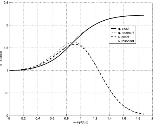
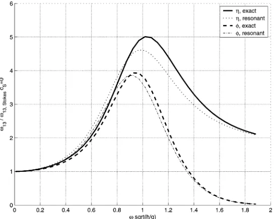
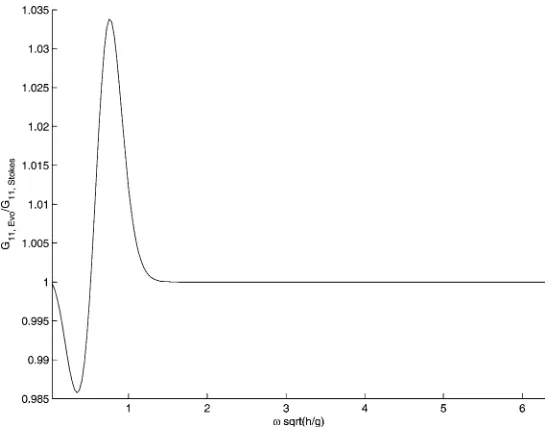
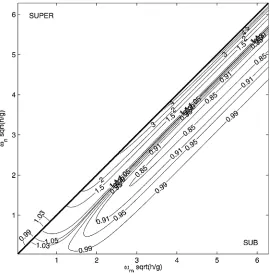
[image:12.544.138.414.441.660.2]Next, we compare the transfer functions of the ‘resonant’ model to the exact transfer functions. We here focus on uni-directional wave propagation. In Fig. 2,GEvo11 , the transfer function for self-self interaction, is plotted against dimensionless angular frequencyω(h/g)1/2for the ‘resonant’ model. The result is normalised with the exact transfer function (57). The trans-fer function is remarkably close to the retrans-ference solution, the largest deviation being an over-prediction of 3.5% at intermediate depth. The full range of bichromatic transfer, still for unidirectional wave propagation is examined in Fig. 3, where the ratio betweenGEvon,mandGStokesn,m is plotted for(ωn(h/g)1/2, ωm(h/g)1/2)∈ [0;2π]2. The super harmonic transfer of the evolution equations is very close to the target of Stokes theory. The small variation observed for the self-self interaction is seen as two small curves close to the diagonal. The reason for the good agreement in the super-harmonic region is thatF(2)s,p−sdecays to zero
Fig. 3. Second-order bichromatic transfer functions for evolution equations invoking the resonance assumption. The values are normalised with the exact transfer function.
for large forcing frequencies. Hence the transfer is dominated by the first term inWs,p−swhich does not involve the H operator. The sub-harmonic transfer is under-predicted in a region parallel to the diagonal and over-predicted along the diagonal. Lines being parallel to the diagonal represent constant receiving frequencies. Parallel lines close to and below the diagonal represent long waves forced sub-harmonically by waves having close frequencies.
5. Speeding up the calculations using FFT
The computational effort of a direct evaluation of the right-hand side of (53) is O(M2N2). For a large number of frequencies (corresponding to a long time series) or a large number ofywave modes, this makes the model infeasible to apply. This problem has traditionally limited the use of evolution equations of the above type.
For the one-dimensional Boussinesq evolution equations of Madsen and Sorensen [7], Bredmose et al. [14] showed that the nonlinear terms can be calculated using Fast Fourier Transforms at a computational effort of O(NlogN ). This method of speeding up the calculation of a convolution sum has been used extensively within spectral methods for partial differential equations, see e.g. Canuto, Hussaini, Quarteroni and Zang [30]. In the field of evolution equations, Dalrymple et al. [25] used this technique to calculate a term corresponding to the second term on the right-hand side of (44). This term is associated with the non-uniformity of depth in the lateral direction. However, for treatment of the nonlinear terms within spatial evolution equations for wave propagation, this speed-up technique appears to be new. Unfortunately, this method of speeding up the calculations cannot be applied directly to the new ‘exact’ models. We detail this later in this section. First, however, we describe the method of the numerical speed-up for the ‘resonant’ models.
Consider the very first term in the nonlinear sums of (53)
term1=iε N
s=p−N
min{l+M,M} t=max{l−M,−M}
¯
kxs,t g
2ωsωp−s
¯
ks,t· ¯kp−s,l−tas,tap−s,l−t
×e−i
(k¯x
s,t+¯kpx−s,l−t−¯kxp,l)dx
For simplicity we evaluate the dot product of the two wave number vectors, and consider only the first term arising. The other term can be treated similarly as the first—as is also the case for all the other terms in the convolution sums. We write the new term as
term11=iε
g
2e
ik¯p,lx dx N s=p−N
min{l+M,M} t=max{l−M,−M}
(k¯x s,t)2
ωs
as,te−i
¯
ks,tx dx k¯x
p−s,l−t
ωp−s
ap−s,l−te−i
¯
kxp−s,l−tdx
. (69)
Inspired by this expression, we define
s1= N
p=−N M
l=−M
(k¯x p,l)2
ωp
ap,le−i
¯
kp,lx dx
eipωte−ik
y
ly, (70)
s2=
N
p=−N M
l=−M
k¯x p,l
ωp
ap,le−i
¯
kxp,ldx
eipωte−ik
y
ly. (71)
which are functions oftandy. Further, we define the Fourier amplitudes of their product as
s1s2≡ 2N
p=−2N 2M
l=−2M
[s1s2]p,leipωteik
y
ly. (72)
The convolution theorem then states that the double summation in (69) is equal to[s1s2]p,l, and we thus have term11=iε
g
2[s1s2]p,le ik¯x
p,ldx. (73)
This is the key point of the speed-up technique. Given the values ofap,l for 1pN and−MlM, and the associated wave numbers and angular frequencies,s1ands2can be calculated by an inverse Fourier transformation in they-direction followed by an inverse Fourier transformation in time. This gives the values ofs1ands2on a grid in the(y, t)plane, and the products1s2can be calculated for each(y, t). Applying two forward Fourier transformations, one in time and one in the
y-direction then gives the values of[s1s2]p,lneeded. If all Fourier transformations are carried out using FFTs, term11can thus be calculated with a computational effort of O((MlogM)(NlogN )). The same procedure can be applied to all the other terms in the ‘resonant’ versions of the models (53) and (44). The second term on the right-hand sides of these models can be treated similarly, although less complicated, since it only involves a single convolution.
As can be seen in (72), the quadratic terms contain Fourier components with frequencies up to double as large as those described in the spectrum resolved. As these higher frequencies do not belong to the spectrum resolved, care must be taken to avoid any aliasing from these frequencies onto the frequency range modelled. Aliasing among the frequencies 1, . . . , Nin time and−M, . . . , Min they-direction is avoided if more than 3N points are used for describing the time variation ofs1s2and more than 3M points are used to describe they-variation. Practically, as the FFT algorithm is most efficient for signal lengths being a product of small prime factors, the number of points in (time,y-direction) should be chosen as the smallest products of this type, exceeding(3N,3M). More details on aliasing can be found in e.g. Canuto et al. [30].
While the above speed-up technique is easily applied to the ‘resonant’ models, it cannot be applied to the ‘exact’ models. The reason is thatH(h∇,k¯p,lh)with∇= −i(k¯s,t+ ¯kp−s,l−t)cannot be written as a product of independent factors, each depending solely on one of the index pairs(p, l),(s, t)and(p−s, l−t)as in (69). It is therefore not possible to define series likes1ands2for an evaluation of the nonlinear terms in the time domain.
Hence, the ‘resonant’ models are more feasible for practical use. We have already found that the second-order transfer for these models is generally close to that of the ‘exact’ models for unidirectional wave propagation. We now validate and compare the models for two test examples.
6. Application to wave propagation over a submerged bar
Fig. 4. Bathymetry and stations for the experiments of Beji and Battjes [15].
6.1. A test on long waves
For the first test, the incident waves are described by a JONSWAP spectrum with a peak frequency of 0.4 Hz and a significant wave height of Hs =2.9 cm. A JONSWAP spectrum (JOint North Sea Wave Project) is a modification of the Pierson–Moscowitz spectrum, see e.g. Sumer and Fredsøe [31]. The time series has a length ofTdur=899.68 s, corresponding to a frequency resolution off1=1/Tdur=1.11×10−3Hz. The wave model (53) in its unidirectional form was run with 1800 frequencies corresponding to a maximum frequency of 2 Hz. The Fourier amplitudes of the experimental time series in station 1 was used as initial condition, and the evolution equations were integrated with a constant spatial step length of 0.1 m. Reducing the step length to 0.05 m had no significant impact on the results. Note that when solving evolution equations, the choice of step length is not governed by a Courant number criterion as for time domain models. If the present test was to be modelled using a time domain model, resolving the shortest wave by two points per wave period would give a time step of 0.25 s. With the current choice of spatial step length of 0.1 m, this would correspond to a Courant number of nearly 5 (!) in the deep part of the domain. This avoidance of the Courant number criterion is one of the reasons for the computational efficiency of evolution equations.
Results from the ‘exact’ model are shown together with experimental time series for stations 3,5 and 8 in Fig. 5. These stations correspond to the two upper corners of the bar and the lower corner after the bar. The time interval depicted represents a typical part of the time series.
The record from station 3 consists of two wave groups with a single isolated wave in between. The high waves have an asymmetric shape, corresponding to a forward leaning of their spatial profiles, resulting from the shoaling process on the bar front. The model results match the data well, except for a few spurious oscillations following the tallest wave crests.
When the waves reach the flat bottom at the bar top, the forward leaning wave shape is no longer stable. The waves change their shape through nonlinear interactions which from a spectral point of view happens through energy exchange between the different frequency components. At the bar top the water is fairly shallow, (kh=0.32 for the peak frequency) and the quadratic interactions therefore approach near-resonance, (see e.g. Phillips [3]). As a result the shape of the waves changes rather dramatically over the bar top. In station 5, the recorded waves are thus seen to be more spiky when compared to station 3 and do not show much asymmetry. The numerical results reproduce the data well, although for the highest waves the crests are seen to be followed by a spurious trough. The highest waves also exhibit small phase errors, the numerical waves arriving slightly too early.
On the down-hill side of the bar, the waves are subject to de-shoaling. In this process some of the high-frequency content of the waves is released as free harmonics, thus resulting in a higher content of high-frequency wave energy behind the bar than in front of the bar. This is clearly seen in the time series of station 8, were the typical wave period is apparently half the period of the waves seen in station 3. The numerical model results exhibit this behaviour as well. Some of the waves are reproduced with reasonable accuracy, while for other waves, phase errors and amplitude errors are seen. In general, the wave model gives a fair reproduction of the overall wave pattern.
Fig. 5. Time series in three stations for the long wave test of Beji and Battjes [15]. Experimental data and results of ‘exact’ model.
Fig. 6. Time series in three stations for the long wave test of Beji and Battjes [15]. Experimental data and results of linearised model.
Fig. 7. Time series in three stations for the long wave test of Beji and Battjes [15]. Comparison between ‘exact’ and ‘resonant’ model.
[image:16.544.77.471.454.594.2]Fig. 8. Time series in three stations for the short wave test of Beji and Battjes [15]. Experimental data and results of ‘exact’ model.
Fig. 9. Time series in three stations for the short wave test of Beji and Battjes [15]. Experimental data and results of linearised model.
6.2. Shorter waves
For the second test chosen, the incoming wave spectrum is a JONSWAP spectrum with a peak frequency of 1 Hz and a significant wave height of 4.1 cm. The duration of the time series isTdur=899.68 s and the evolution equations were solved with 2700 frequencies, corresponding to a maximum frequency of 3 Hz.
First we examine the results for the time intervalt= [490;520]s. Results of the ‘exact’ model are compared to experimental data in Fig. 8, while results of a linear model run are compared to data in Fig. 9. In general, both models are able to capture the individual waves. However, the waves calculated with the nonlinear evolution equations show a forward phase shift when compared to the data. This phase shift is not present for the linear results and is thus a consequence of nonlinearity. In station 5, the results of the linear model in general exhibit too deep wave troughs. This behaviour is not seen for the results of the nonlinear evolution equations, although for this station the phase shift has increased due to accumulative effects. For station 8, both models reproduce the overall variation of the wave field, although phase errors and spurious high-frequency oscillations are present in the results.
We now focus on the results for a single tall wave group, covering the time intervalt= [325;340]s. Numerical results of the nonlinear evolution equations are compared to the measured time series in Fig. 10, while linear results and data are compared in Fig. 11. For station 3, the asymmetry and spikiness of the measured waves indicate the presence of second harmonic energy in the wave spectrum. The nonlinear evolution equations capture the appearance of the second harmonics and thus reproduce the shape of the waves with a good improvement from linear theory. The same holds for the results of station 5. For these stations phase errors are evident for both models, the linear model results exhibiting a backward phase shift and the nonlinear model exhibiting a forward phase shift in time. This shows that there is a nonlinear contribution to the phase speed in the data, and that the nonlinear model overestimates this contribution. For station 8, these phase shifts accumulate for both models and thus make a judgement of the reproduction of wave shape difficult.
Fig. 10. Time series in three stations for the short wave test of Beji and Battjes [15]. Experimental data and results of ‘exact’ model.
Fig. 11. Time series in three stations for the short wave test of Beji and Battjes [15]. Experimental data and results of linearised model.
Fig. 12. Time series in three stations for the short wave test of Beji and Battjes [15]. Results of ‘exact’ model and ‘resonant’ model.
the measured data is relatively large. From a modelling point of view, the results of the two models can therefore be considered of equal quality for this test case.
[image:18.544.76.476.445.585.2]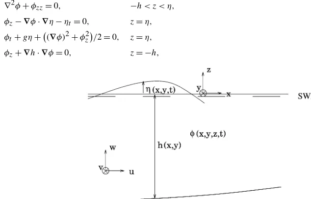
![Fig. 4. Bathymetry and stations for the experiments of Beji and Battjes [15].](https://thumb-us.123doks.com/thumbv2/123dok_us/8140338.244758/15.544.140.407.66.183/fig-bathymetry-stations-experiments-beji-battjes.webp)
![Fig. 5. Time series in three stations for the long wave test of Beji and Battjes [15]](https://thumb-us.123doks.com/thumbv2/123dok_us/8140338.244758/16.544.77.471.454.594/fig-time-series-stations-long-wave-beji-battjes.webp)
![Fig. 8. Time series in three stations for the short wave test of Beji and Battjes [15]](https://thumb-us.123doks.com/thumbv2/123dok_us/8140338.244758/17.544.77.471.71.215/fig-time-series-stations-short-wave-beji-battjes.webp)
![Fig. 10. Time series in three stations for the short wave test of Beji and Battjes [15]](https://thumb-us.123doks.com/thumbv2/123dok_us/8140338.244758/18.544.76.476.445.585/fig-time-series-stations-short-wave-beji-battjes.webp)