Exotic equity options

(1)

Exotic equity options

Dr. Graeme West

Financial Modelling Agency

graeme@ﬁnmod.co.za

(2)

Review of distributions and statistics

For this course, we will value equity options in the risk neutral world where we have

𝑑𝑆= (𝑟−𝑞)𝑆 𝑑𝑡+𝜎𝑆 𝑑𝑍 (1.1)

where the time is measured in years. One of the most important factors of this formulation is that the risk free rate, the dividend yield, and the volatility are all constant. Whilst the risk free and the dividend yield assumptions are not too problematic (in an equity derivative environment), the volatility assumption is untenable. Volatility is certainly a function of time (this part is quite easy) but is also a function of how the stock price evolves: so𝜎=𝜎(𝑆, 𝑡), which is called the local volatility. Models of the volatility skew or smile are thus crucial. The development of the theory has branched into local volatility models and stochastic volatility models, with the latter now predominant theoretically but the former still in heavy use (although theoretically inferior, they are computationally almost instantaneous, whereas stochastic volatility pricing almost always reduces to Monte Carlo). The key evolution isDupire[1994],Dupire[1997],Derman[1999],Derman and Kani

[1998], Heston [1993], Hull and White [1987], Fouque et al. [2000], Hagan et al. [2002]. In all cases, vanilla options and the vanilla skew are used to calibrate the model, which is then used for pricing of exotic options. But, for the rest of this course, we will assume that volatility is constant, or (at the worst) that it has a term structure. Only in some speciﬁc instances will we allow volatility to be dependent on the strike or on the evolution of spot, and we don’t allow for jumps in the stock price (the stock price is a diﬀusion).

1.1 Distributional facts

A basic statistical result we shall use repeatedly is that if the random variable𝑍has probability density function

𝑓, and𝑔 is a suitably deﬁned function then

𝔼[𝑔(𝑍)] =

∫

𝑓(𝑠)𝑔(𝑠)𝑑𝑠 (1.2)

where the integration is done over the domain of𝑓. This allows us to work out_𝔼[𝑍] and_𝔼[ 𝑍2]

(6)

Now, note from statistics that if𝑋 = ln𝑊 ∼𝜙(Ψ,Σ) 1 _{then the relevant probability density functions are}

𝑓𝑋(𝑥) =

1

√

2𝜋Σexp

[

−1 2

(𝑥−Ψ)2

Σ

]

(1.3)

𝑓𝑊(𝑥) =

1

√

2𝜋Σ𝑥exp [

−1 2

(ln𝑥−Ψ)2

Σ

]

(1.4)

Of course the domain for𝑓𝑋 isℝwhile the domain for𝑓𝑊 is (0,∞).

In the risk neutral formulation above, by Itˆo’s lemma

𝑋 := ln

(_𝑆₍_𝑇₎ 𝑆(𝑡)

)

∼𝜙 ((

𝑟−𝑞−𝜎

2

) 𝜏, 𝜎2𝜏

)

(1.5)

Note now that𝑆(𝑇) =𝑆(𝑡)𝑒𝑋: a very useful representation for European derivatives. Let

𝑚±=𝑟−𝑞± 𝜎2

2 (1.6)

So𝑋∼𝜙(𝑚−𝜏, 𝜎2𝜏) and so the probability density function for 𝑋 is

𝑓(𝑥) =√ 1

2𝜋𝜎√𝜏exp [

−1 2

(𝑥−𝑚−𝜏)2 𝜎2_𝜏

]

(1.7)

and the probability distribution for𝑆(𝑇) is

𝑓(𝑥) =√ 1

2𝜋𝜎√𝜏 𝑥exp [

−1 2

(ln𝑥−ln𝑆(𝑡)−𝑚−𝜏)2 𝜎2_𝜏

]

(1.8)

Now if ln𝑌 ∼𝜙(Ψ,Σ) then for𝑘 >0

𝔼[𝑌𝑘] =

1

√

2𝜋Σ

∫ ∞

−∞ 𝑒𝑘𝑥exp

[

−1 2

(𝑥−Ψ)2

Σ

] 𝑑𝑥

= exp( 𝑘Ψ +1

2𝑘 2_Σ)

(1.9)

which will be crucial in Chapter10. Thus in the above risk neutral setting we have

𝔼ℚ𝑡

[ 𝑆(𝑇)𝑘]

=𝑆(𝑡)𝑘exp((

𝑘(𝑟−𝑞) +1₂(𝑘2−𝑘)𝜎2)𝜏)

(1.10)

The ﬁrst derivative of the cumulative normal

This is the closed form formula:

𝑁′(𝑥) =√1

2𝜋𝑒 −𝑥2_/₂

(1.11)

The second derivative of the cumulative normal

This is again, given by a closed form formula:

𝑁′′(𝑥) =−𝑥𝑁′(𝑥) (1.12)

1_{By this we mean that the mean is Ψ and the variance is Σ. This could apply to more than one dimension too, in which case}

Ψ would be the mean vector and Σ the covariance matrix. Furthermore, in general we reserve the symbol𝜎 for the annualised volatility, also known as the volatility measure, and do not use it as the standard deviation of some distribution.

(7)

The inverse of the cumulative normal

Given an input 𝑦, the Inverse Standard Normal Integral gives the value of 𝑥for which 𝑁(𝑥) =𝑦, where𝑁(⋅) denotes the Cumulative Standard Normal Integral.

The Moro transformMoro[February 1995] to ﬁnd this function is the most well known algorithm. Having the ability to generate normally distributed variables from a (quasi) random uniform sample is clearly important in work involving any Monte Carlo experiments, and the Moro transformation is fast and accurate to about 10 decimal places.

For another approach, we can use our existing cumulant function and any version of Newton’s method. As pointed out in Acklam [2004], having a double precision function has some rather pleasant spin-offs. Given a function that can compute the normal cumulative distribution function to double precision, the Moro ap-proximation of the inverse normal cumulative distribution function can be refined to full machine precision, by a fairly straightforward application of Newton’s method. In fact, higher degree methods such as Newton’s second order method (sometimes called the Newton-Bailey method) or a third order method known as Halley’s method will be the fastest, and are very amenable here, because the Gaussian function is so easily differentiated over and over - seeAcklam [2004] andAcklam[2002].

The Newton-Bailey method would be as follows:

𝑥𝑛+1 = 𝑥𝑛−

𝑓(𝑥𝑛)−𝑦

𝑓′₍_𝑥

𝑛)−(𝑓(𝑥𝑛)−𝑦)𝑓

′′₍_𝑥

𝑛)

2𝑓′₍_𝑥

𝑛)

= 𝑥𝑛−

𝑓′₍_𝑥

𝑛) +

(𝑓(𝑥𝑛)−𝑦)𝑥𝑛𝑓′(𝑥𝑛)

2𝑓′₍_𝑥

𝑛)

= 𝑥𝑛−

𝑓′₍_𝑥

𝑛) +1₂(𝑓(𝑥𝑛)−𝑦)𝑥𝑛

Earlier versions of excel had an absurd error in the NORMSINV function: it would return impossible values for inputs within 0.0000003 of 1 or 0 respectively. Given that such values close to 0 or 1 on occasion are provided by uniform random number generators, this approach is to be avoided. Also note that the random number generator rand()/rnd() in excel/vba is absurd as it can (and does) return the value 0 and 1. This will cause either your own inverse function, or NORMSINV, to fail.

1.2 Risk Neutral Probabilities

We can speed up and simplify the calculation of the risk-neutral probabilities in option premium formulae. As usual in option pricing, we have

𝜏 = 𝑇−𝑡

𝑑± =

ln_𝐾𝑓 ±1 2𝜎

2_𝜏

𝜎√𝜏

where𝑓 denotes the forward level for spot-type options and the futures level for options involving futures. Certain special cases apply, where the formula does not make sense in a pure sense, but can be made sense of mathematically by taking limits. This occurs if any of forward/future, strike, term or volatility are zero. The appropriate outcome in these cases (in the sense of a limit) is determined by testing:

• when the strike𝐾 is zero,𝑑±=∞which will give𝑁(𝑑±) = 1 and𝑁′(𝑑±) = 0,

(8)

• when either term or volatility are zero, and𝑓 is greater than the strike,𝑑± =∞which will give𝑁(𝑑±) = 1

and𝑁′(𝑑±) = 0,

• when either term or volatility are zero, and𝑓 is less than the strike,𝑑±=−∞which will give𝑁(𝑑±) = 0

and𝑁′(𝑑±) = 0.

1.3 Bivariate cumulative normal

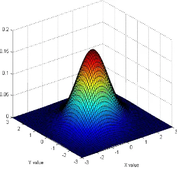
The probability density function of the bivariate normal distribution is

𝜙2(𝑋, 𝑌, 𝜌) = 1

2𝜋√1−𝜌2exp

[₋₍_𝑋2₋₂_𝜌𝑋𝑌 ₊_𝑌2₎

2(1−𝜌2₎ ]

(1.13)

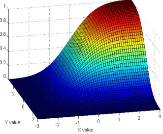
The cumulative bivariate normal distribution is the function

𝑁2(𝑥, 𝑦, 𝜌) = 1 2𝜋√1−𝜌2

∫ 𝑥 −∞ ∫ 𝑦 −∞ exp [

−(𝑋2₋₂_𝜌𝑋𝑌 ₊_𝑌2₎

2(1−𝜌2₎ ]

𝑑𝑌 𝑑𝑋 (1.14)

Again, approximations are required. The most common algorithm is that ofDrezner[1978], which appears in both [Hull,2002, Appendix 12C] and in [Haug,1998, Appendix A.2], for example.

We have adapted one of the algorithms fromGenz[2004], namely, the modiﬁcation of the algorithm ofDrezner and Wesolowsky[1989]. This algorithm tests against the previous independent implementations, and it can be veriﬁed using numerical integration that it is accurate to at least 14 decimal places.

Adaptation was needed because the algorithm calculated the complementary probability that𝑋 ≥𝑥, 𝑌 ≥𝑦

given the correlation coeﬃcient. The algorithm has been adapted to return the more usual probability that

𝑋 ≤𝑥,𝑌 ≤𝑦.

Limiting cases are important for the bivariate cumulative normal. Note that in the sense of a limit

𝑁2(𝑥, 𝑦,1) = 𝑁(min(𝑥, 𝑦)) (1.15)

𝑁2(𝑥, 𝑦,−1) =

{

0 if 𝑦≤ −𝑥

𝑁(𝑥) +𝑁(𝑦)−1 if 𝑦 >−𝑥 (1.16)

We have that

∂

∂𝑥𝑁2(𝑥, 𝑏, 𝜌) = ∂ ∂𝑥

1 2𝜋√1−𝜌2

∫ 𝑥 −∞

∫ 𝑏 −∞

exp

[₋₍_𝑋2₋₂_𝜌𝑋𝑌 ₊_𝑌2₎

2(1−𝜌2₎ ]

𝑑𝑌 𝑑𝑋

= 1

2𝜋√1−𝜌2 ∫ 𝑏

−∞

exp

[

−(𝑥2−2𝜌𝑥𝑌 +𝑌2) 2(1−𝜌2₎

] 𝑑𝑌

=𝑁′(𝑥)𝑁 (

𝑏−𝜌𝑥 √

1−𝜌2 )

(1.17)

and hence by the Fundamental Theorem of Calculus

∫ 𝑎 −∞

𝑁′(𝑥)𝑁 (

𝑏−𝜌𝑥 √

1−𝜌2 )

𝑑𝑥=𝑁2(𝑎, 𝑏, 𝜌)

by manipulating with the constants we get

∫ 𝑎 −∞

𝑁(𝐾+𝐿𝑥)𝑁′(𝑥)𝑑𝑥=𝑁2 (

𝑎,√ 𝐾

𝐿2_{+ 1},

−𝐿

√

𝐿2_{+ 1} )

(9)

[image:9.612.128.493.147.495.2]

Figure 1.1: The bivariate normal pdf

It follows by completing the square from this that

∫ 𝑎 −∞

𝑒𝐴𝑥𝑁(𝐾+𝐿𝑥)𝑁′(𝑥)𝑑𝑥=𝑒𝐴 2 2 𝑁2

(

𝑎−𝐴, √𝐾+𝐴𝐿

𝐿2_{+ 1},

−𝐿

√

𝐿2_{+ 1} )

(1.19)

1.4 Trivariate cumulative normal

The cumulative trivariate normal distribution is the function

𝑁3(𝑥1, 𝑥2, 𝑥3,Σ) =

1 (2𝜋)3/2√

∣Σ∣

∫ 𝑥1 −∞

∫ 𝑥2 −∞

∫ 𝑥3 −∞

exp(

−1 2𝑋

′_Σ−1_𝑋)

(10)

[image:10.612.147.478.140.413.2]

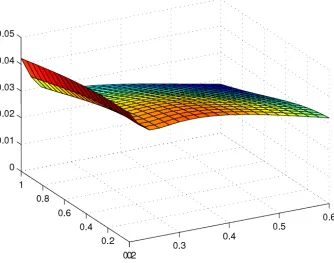
Figure 1.2: The bivariate cumulative normal function,𝜌= 50%

where Σ is the correlation matrix between standardised (scaled) variables𝑋1,𝑋2,𝑋3, and ∣ ⋅ ∣denotes

deter-minant. Denote by 𝑁3(𝑥1, 𝑥2, 𝑥3, 𝜌21, 𝜌31, 𝜌32) the function 𝑁3(𝑥1, 𝑥2, 𝑥3,Σ) where Σ =

⎡

⎢ ⎣

1 𝜌21 𝜌31 𝜌21 1 𝜌32 𝜌31 𝜌32 1

⎤

⎥ ⎦.

Again, approximations are required. Code for the trivariate cumulative normal is not generally available. There are a few highly non-transparent publications, for exampleSchervish[1984], but this code is known to be faulty. We have used the algorithm inGenz[2004]. This has required extensive modiﬁcations because the algorithms are implemented in Fortran, using language properties which are not readily translated. The function inGenz

[2004] returns the complementary probability, again, we have modiﬁed to return the usual probability that

𝑋𝑖 ≤𝑥𝑖 (𝑖= 1,2,3) given a correlation matrix. Again, it is claimed that this algorithm is double precision;

high accuracy (of our vb and c++ translations) has been veriﬁed by testing against Niederreiter quasi-Monte Carlo integration (using the Matlab algorithm qsimvn.m, also at the website of Genz).

As before, one can show that

𝑁3(𝑥1, 𝑥2, 𝑥3,Σ) = ∫ 𝑥3

−∞

𝑁′(𝑥)𝑁2 (

𝑥1−𝜌13𝑥 √

1−𝜌2 13

,𝑥2_√−𝜌23𝑥

1−𝜌2 23

,_√ 𝜌12−𝜌13𝜌23

1−𝜌2 13

√

1−𝜌2 23

)

𝑑𝑥 (1.21)

Many of the issues surrounding developing robust code for these cumulative functions are discussed in West

(11)

1.5 Exercises

1. Write vba code for the Newton-Bailey method of ﬁnding the cumnorm inverse function. Use the double precision cumnorm function provided. Use ‘newx’ below as your ﬁrst estimate, where ‘y’ is the input:

r = Sqr(-2 * Log(Min(y, 1 - y)))

newx = r - (2.515517 + 0.802853 * r + 0.010328 * r ˆ 2) /

(1 + 1.432788 * r + 0.189269 * r ˆ 2 + 0.001308 * r ˆ 3)

If y < 0.5 Then newx = -newx

2. Show that if𝑆 is subject to GBM with drift𝜇and volatility𝜎,

𝔼[𝑆(𝑇)𝑘] =𝑆(𝑡)𝑘exp((𝑘𝜇+12(𝑘 2

−𝑘)𝜎2)(𝑇−𝑡))

3. Formally verify (1.15) and (1.16).

4. Verify (1.17), (1.18) and (1.19).

5. Find the integral∫_𝛼∞⋅ ⋅ ⋅ in place of (1.18).

6. (exam 2004) Consider the bivariate normal cumulative function𝑁2(𝑥, 𝑦, 𝜌). Recall this is the probability

that𝑋 ≤𝑥,𝑌 ≤𝑦where𝑋and𝑌 are normally distributed variables which are correlated with correlation coeﬃcient𝜌. So

𝑁2(𝑥, 𝑦, 𝜌) =

∫ 𝑥 −∞

∫ 𝑦 −∞

𝑓(𝑋, 𝑌, 𝜌)𝑑𝑌 𝑑𝑋

where 𝑓 is the relevant probability density function. Let𝑀2(𝑥, 𝑦, 𝜌) be the complementary probability i.e. it is the probability that 𝑋 ≥𝑥, 𝑌 ≥𝑦. Also𝑁(⋅) is the usual cumulative normal function. Prove that

(12)

Chapter 2

Structures

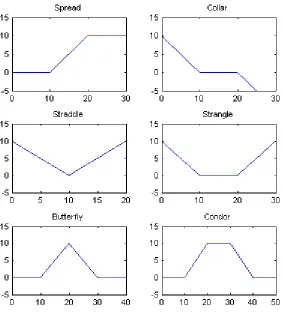
Any piecewise linear payoff can be decomposed into some linear combination of (calls, puts,) asset or nothing and cash or nothing options. Although there are theorems that deal with this, their notational complexity conceals the fact that the procedure one needs to invoke is fairly routine. First, we will see some of the ideas in play in typical option payoff profiles.

2.1 Spreads

A spread (vertical) has options at two strikes at the same expiry date on the same stock. The options are either both calls or both puts, with one long and the other short.

• A bull call spread is long the call at the lower strike and short the call at the higher strike.

• A bear call spread is short the call at the lower strike and long the call at the higher strike.

• A bull put spread is long the put at the lower strike and short the put at the higher strike.

• A bear put spread is short the put at the lower strike and long the put at the higher strike.

2.2 Collars

Suppose we have a long position in stock. We might want to avoid massive losses in the event that the stock price falls dramatically by buying an out the money put. Rather than paying for the put, we sell an out the money call to the same counterparty. This structure is called a collar. To emphasise that there is no premium, it is sometimes called a zero-cost collar.

Similarly if we have a short position in the stock we might go long an out the money call and short an out the money put.

Such a zero-cost collar might be called a range forward, a cylinder or a tunnel.

2.3 Straddles and strangles

(13)

• A strangle is long 1 call at a higher strike and long 1 put at a lower strike in the same expiration and on the same stock.

Such long positions makes money if the stock price moves up or down well past the strike prices of the strangle. Long straddles and strangles have limited risk but unlimited proﬁt potential.

Such short positions makes money if the stock price stays at or about the strike(s). Short straddles and strangles have unlimited risk and limited proﬁt potential.

2.4 Butterﬂies and condors

• A butterﬂy is long a call at strike𝑋1, short two calls at𝑋2, and long a call at𝑋3, with𝑋3−𝑋2=𝑋2−𝑋1.

• A condor (wingspread) has options at four strikes, with the same distance between the each wing strike and the lower or higher of the body strikes. Thus, a call is long a call at strike𝑋1, short one call at𝑋2,

short a call at 𝑋3, and long a call at𝑋4, with𝑋4−𝑋3=𝑋2−𝑋1 and𝑋3> 𝑋2.

[image:13.612.173.456.365.686.2]

The identical structure can be manufactured with puts instead of calls!

(14)

Chapter 3

Review of vanilla option pricing

3.1 Deriving the Black-Scholes formula

By the principle of risk-neutral valuation, the value of a European call option is

𝑉 =𝑒−𝑟𝜏 _𝔼ℚ

𝑡

[

max(𝑆𝑒𝑋−𝐾,0)]

(3.1)

where𝑋 has the meaning of (1.5). We now calculate:

𝑉 = 𝑒−𝑟𝜏 _𝔼ℚ

𝑡

[

max(𝑆𝑒𝑋−𝐾,0)]

= 𝑒−𝑟𝜏√ 1

2𝜋𝜎√𝜏 ∫ ∞

−∞

max(𝑆𝑒𝑥−𝐾,0) exp

[

−1 2

(

𝑥−𝑚−𝜏 𝜎√𝜏

)2] 𝑑𝑥

= 𝑒−𝑟𝜏√ 1

2𝜋𝜎√𝜏 ∫ ∞

ln𝐾 𝑆

(𝑆𝑒𝑥−𝐾) exp

[

−1 2

(_𝑥

−𝑚−𝜏 𝜎√𝜏

)2] 𝑑𝑥

= 𝑒−𝑟𝜏𝑆√ 1

2𝜋𝜎√𝜏 ∫ ∞

ln𝐾 𝑆

𝑒𝑥exp

[

−1 2

(_𝑥₋_𝑚 −𝜏 𝜎√𝜏

)2] 𝑑𝑥

−𝑒−𝑟𝜏𝐾√ 1

2𝜋𝜎√𝜏 ∫ ∞ ln𝐾 𝑆 exp [ −1 2

(_𝑥₋_𝑚 −𝜏 𝜎√𝜏

)2] 𝑑𝑥

Now, for the ﬁrst integral, we complete the square:

𝑥−1 2

(

)2

= 𝑥−1 2

𝑥2₋₂_𝑚

−𝜏 𝑥+𝑚2−𝜏2 𝜎2_𝜏

= −1 2

𝑥2₋₂_𝑚

−𝜏 𝑥−2𝑥𝜎2𝜏+𝑚2−𝜏2 𝜎2_𝜏

= −1 2

𝑥2₋₂_{𝑚+𝜏 𝑥}₊_𝑚2 −𝜏2 𝜎2_𝜏

= −1 2

(𝑥−𝑚+𝜏)2−𝑚2+𝜏2+𝑚2−𝜏2 𝜎2_𝜏

= −1 2

(_𝑥₋_𝑚+𝜏

𝜎√𝜏 )2

(15)

so

𝑉 = 𝑒−𝑞𝜏𝑆√ 1

2𝜋𝜎√𝜏 ∫ ∞

ln𝐾 𝑆

exp

[

−1 2

(_𝑥₋_𝑚+𝜏

𝜎√𝜏 )2]

𝑑𝑥

−𝑒−𝑟𝜏𝐾√ 1

2𝜋𝜎√𝜏 ∫ ∞

ln𝐾 𝑆

exp

[

−1 2

(

)2] 𝑑𝑥

= 𝑒−𝑞𝜏𝑆𝑁 (

𝑚+𝜏−ln𝐾_𝑆

𝜎√𝜏 )

−𝑒−𝑟𝜏𝐾𝑁 (

𝑚−𝜏−ln𝐾_𝑆

𝜎√𝜏 )

= 𝑒−𝑞𝜏𝑆𝑁(𝑑+)−𝑒−𝑟𝜏𝐾𝑁(𝑑−)

where the meaning of𝑑+and𝑑− will be established now.

The put formula follows by put-call parity, or by mimicking the argument.

3.2 Vanilla pricing methods for equity options

Note that in all cases

𝑉 = 𝜉𝜂[f𝑁(𝜂𝑑+)−𝐾𝑁(𝜂𝑑−)] (3.2)

𝑑± =

ln(f/𝐾)±1 2𝜎

2_𝜏

𝜎√𝜏 (3.3)

where

• 𝜉is𝑒−𝑟𝜏 _{for an European Equity Option and for Standard Black, and 1 for SAFEX Black Futures Options}

and SAFEX Black Forward Options.

• 𝜂= 1 for a call and𝜂 =−1 for a put,

• f =𝑓 =𝑆𝑒(𝑟−𝑞)𝜏 _{is the forward value for an European Equity Option and for SAFEX Black Forward}

Options, andf =𝐹 is the futures value for Standard Black and SAFEX Black Futures Options.

3.3 A more general result

In full generality, we have the following result.

Lemma 3.3.1. Suppose we have a vanilla European call or put on a variable𝑌, strike𝐾, where the terminal value of𝑌 is lognormally distributed, log𝑌 ∼𝜙(Ψ,Σ). Then the option price is given by

𝑉𝜂 = 𝑒−𝑟𝜏𝜂

[

𝑒Ψ+12Σ𝑁(𝜂𝑑+)−𝐾𝑁(𝜂𝑑−) ]

(3.4)

𝑑+ = Ψ + Σ√−log𝐾

Σ (3.5)

𝑑− =

Ψ−log𝐾

√

Σ (3.6)

(16)

3.4 Implied volatility

For any of the 4 option types we will on occasion know all of the inputs except the volatility, and know the premium, and require the volatility that, when input, will return the correct premium. Such a volatility is known as the implied volatility. It can be found using the Newton-Rhapson method, although one has to be careful, because an injudicious seed value will cause this method to not converge. In Manaster and Koehler

[1982], a seed value of the implied volatility is given which guarantees convergence.

The argument inManaster and Koehler[1982] is unnecessarily complicated, and can easily be understood as follows: premium as a function of volatility is an increasing function, bounded below by the intrinsic value and above by the price of the underlying. It is initially convex up and subsequently convex down. Thus, choosing the point of inflection as the seed value, guarantees convergence, no matter which way the iteration, which will be monotone and quadratic in speed, will go. By simple calculus, one finds this point of inflection, for any of the four methods, to be

𝜎=

√

2

𝜏

ln 𝑓

𝐾

(3.7)

However, note that this method fails outright if the option is at the money forward.

An alternative to use the first estimate of Corrado and Miller[1996], modified to ensure valid computation. This estimate is the root of a quadratic, but a na¨ıve application will run into the problem of having complex roots. Thus, a first estimate which is always valid is:

𝜎=

√

2𝜋 𝜉(𝑓+𝐾)√𝜏

⎡

⎣𝑉 −𝜉𝜂(𝑓 −𝐾)

2 +

v u u ⎷max

(

0, (

𝑉 −𝜉𝜂(𝑓 −𝐾)

2

)2

−(𝜉(𝑓−𝐾))

2 𝜋

)⎤

⎦ (3.8)

The code will then expand this point to an interval in which the root must lie, and then use Brent’s algorithm.

3.5 Calculation of forward parameters

Forward quantities are calculated as follows:

𝑟(0;𝑇1, 𝑇2) = 𝑟2𝑇2−𝑟1𝑇1

𝑇2−𝑇1

(3.9)

𝑞(0;𝑇1, 𝑇2) = 𝑞2𝑇2−𝑞1𝑇1

𝑇2−𝑇1 (3.10)

𝜎(0;𝑇1, 𝑇2) = √

𝜎2

2𝑇2−𝜎21𝑇1

𝑇2−𝑇1 (3.11)

where time is measured in years. Alternatively, for dividends, we may simply calculate the forward values or the present value of the forward values. For the volatility, this is the at the money volatility. Inclusion of the skew is always tricky and requires additional assumptions.

3.6 Exercises

1. Repeat the derivation of the Black-Scholes formula, this time for puts.

(17)

3. Verify that, with the usual notation, f𝑁′(𝑑1) =𝐾 𝑁′(𝑑2). Torturous, long, solutions are problematic.

That does not mean leave out details!

4. (a) Make sure your cumnorm function is working. Approximately, on what domain does it return values which are diﬀerent from 0 or 1? Why is this not the whole real line?

(b) Write a𝑑1 and a𝑑2 function. Be sure to accommodate the special cases discussed in§1.2.

(c) Write a SAFEX Black option pricing function (inputs 𝐹, 𝐾, 𝜎, valuation date, expiry date and style).

(d) Make sure that the function works for the special cases already discussed. This work should be done by the𝑑𝑖functions, not by the option pricing functions.

(e) Draw graphs of the option values for varying spot/future and varying time to expiry.

(f) Extend to a Black-Scholes option pricing function (inputs𝑆,𝑟,𝑞,𝐾,𝜎, valuation date, expiry date and style).

5. (exam 2004) A supershare option entitles the holder to a payoﬀ of 𝑆_𝑋(𝑇)

𝐿 if 𝑋𝐿 ≤ 𝑆(𝑇) ≤ 𝑋𝐻, and 0

otherwise. The price of a supershare option is given by

𝑉 = 𝑆

𝑋𝐿

𝑒−𝑞𝜏[𝑁(𝑑1)−𝑁(𝑑2)]

𝑑1=

ln_𝑋𝑓

𝐿 +

1 2𝜎

2_𝜏

𝜎√𝜏

𝑑2= ln

𝑓 𝑋𝐻 +

1 2𝜎

2_𝜏

𝜎√𝜏

Create a option pricing calculator in excel, referring to a pricing function written in vba. The time input will be in years i.e. don’t use dates. Draw a spot proﬁle of the value of the derivative.

6. (exam 2004) The Standard Black call option pricing formula is

𝑉 =𝑒−𝑟𝜏(𝐹 𝑁(𝑑1)−𝐾𝑁(𝑑2))

Δ =𝑒−𝑟𝜏𝑁(𝑑1)

Γ =𝑒−𝑟𝜏𝑁′(𝑑1)

1

𝐹 𝜎√𝜏

𝑑1,2=

ln𝐹_𝐾±1 2𝜎

2_𝜏

𝜎√𝜏

(a) Write code to price, and provide Greeks for, a call option using the Standard Black formula. The last input of your list of inputs to the pricing formula will be an optional string parameter. The default will be “p” (for premium). Have “d” (for delta) and “g” (for gamma) other possibilities. Fix the strike, the volatility, the risk free rate, and the term (which will be in years i.e. don’t use dates).

(b) For a range of futures prices, draw graphs (separate sheets for each) of the value, the delta, and the gamma. On each of these above sheets, illustrate the eﬀect of time on each proﬁle by drawing the graphs for 6 months, 1 month and 1 week to expiry.

(18)

8. (a) Write code to price, and provide Greeks for, a European call option using Black-Scholes. The last input of your list of inputs to the pricing formula will be an optional string parameter. The default will be ”p” (for premium). Have ”d” (for delta) and ”g” (for gamma) other possibilities.

(b) For a range of spot prices, draw graphs (separate sheets for each) of the value, the delta, and the gamma.

(19)

Chapter 4

Dividend yields and discrete dividends

Typically European equity options are priced using the Black-Scholes modelBlack and Scholes[1973] or that model adjusted for dividends by calculating a continuous dividend yield. This has the eﬀect of spreading the dividend payment throughout the life of the option. This is most attractive where the option is on an index (where the index is paying out several dividends, spread out through the period of optionality).

For American equity options with the underlying having no or several dividends, we may argue similarly. Here the approximation of Barone-Adesi and WhaleyBarone-Adesi and Whaley[1987] is popular, but we prefer the method of Bjerksund and StenslandBjerksund and Stensland [1993], Bjerksund and Stensland [2002] as it is computationally far superior, and has been shown to be more accurate in long dated options.

Bjerksund and Stensland[2002] is a more recent improvement overBjerksund and Stensland[1993].

Another standard approach (for the European case) is to reduce the stock value by the present value of dividends (the escrowed dividend method), or to increase the strike by the future value of dividends. Both are unsatisfactory approaches as they aﬀect the stochastic process on the equity fairly signiﬁcantly. See Frishling

[2002],Bos and Vandermark[2002],Haug et al.[2003].

In the case of only a few dividend payments on the underlying equity, the original approach above - calculating a continuous dividend yield and using that in a closed form formula - is also no longer satisfactory, even for European options. The dividends occur at one or a few discrete times, but we are spreading them out throughout the life of the option by making this assumption, and this has a material eﬀect on the stochastic process for the stock price.

This comment also applies to the classic binomial tree approach for pricing American options developed in

Cox et al.[1979]. Use of a binomial tree necessitates that risk free rates are assumed constant, and that there is a constant dividend yield, as described above. This will lead to the same severe problems as before. Note that dividends cannot be made discrete in the tree approach because doing so will make the tree no longer recombine, which is computationally a disaster.

(20)

price has decreased somewhat, the company will attempt to maintain dividend levels at more or less the same currency level, at least for a while. Thus, the model that dividends are a known proportion of share price is not practicable.

The most meaningful possibility is that the ﬁrst few dividends are known or predicted in cash, whilst the remaining dividends are predicted as a proportion of stock price. Our preferred approach is as follows: use broker/analyst forecasts in the short and medium term, and then forecast percentage dividends in the long term using the model of [West,2009,§6.6]. Alternatively, if there are no broker forecasts (for a smaller stock, or simply because we are operating under informational constraints) then all forecasts are percentage dividends based on history.

In the case of an American call with one dividend, the formula of Roll, Geske, WhaleyRoll[1977],Geske[1979a],

Whaley[1981] is well known (amongst practitioners) to be arbitragable (and not so well known amongst software vendors, who often insist on oﬀering this as the default model). Again, seeFrishling[2002],Haug et al.[2003]. Furthermore, their approach does not allow for the pricing of American puts (as is well known, the pricing of American puts is in general more diﬃcult than the pricing of calls).

Thus, for European or American options with a few dividends, one should probably prefer to use a finite difference scheme for pricing. This finite difference scheme easily accommodates the discrete jumps of dividends, and both the cash and proportion formulation. One can use the finite difference approach for any number of dividends if prepared to input them. As the number of dividends increases, the benefits of these approaches are outweighed by the superior speed of using the continuous dividend yield proxy in the Black-Scholes or Bjerksund-Stensland formula.

4.1 Pricing European options by Moment Matching

Let𝑡=𝑡0with dividends occurring on𝑡1, . . . , 𝑡𝑛 and𝑇 =𝑡𝑛+1. Now if we have a cash dividend𝐷𝑖on𝑡𝑖then

𝑆(𝑡𝑖) =𝑆(𝑡𝑖−1)𝑒𝑋𝑖−𝐷𝑖

⇒𝑆(𝑡𝑖)2=𝑆(𝑡𝑖−1)2𝑒2𝑋𝑖−2𝐷𝑖𝑆(𝑡𝑖−1)𝑒𝑋𝑖+𝐷2𝑖

and so

𝔼[𝑆(𝑡𝑖)] =𝔼[𝑆(𝑡𝑖−1)]𝔼[𝑒𝑋𝑖]−𝐷𝑖

𝔼

[ 𝑆(𝑡𝑖)

2]

=_𝔼[𝑆(𝑡𝑖−1)2 ]

𝔼[𝑒2𝑋𝑖]−2𝐷𝑖𝔼[𝑆(𝑡𝑖−1)]𝔼[𝑒𝑋𝑖]+𝐷𝑖2.

Here𝑋𝑖= ln

( _𝑆₍_𝑡−

𝑖)

𝑆(𝑡𝑖−1)

)

and we know its distribution as in (1.5). Otherwise, if we have a simple dividend yield𝑑𝑖, then

𝑆(𝑡𝑖) =𝑆(𝑡𝑖−1)𝑒𝑋𝑖(1−𝑑𝑖)

⇒𝑆(𝑡𝑖)2=𝑆(𝑡𝑖−1)2𝑒2𝑋𝑖(1−𝑑𝑖)2

so that

𝔼[𝑆(𝑡𝑖)] =𝔼[𝑆(𝑡𝑖−1)]𝔼[𝑒𝑋𝑖](1−𝑑𝑖)

𝔼

[ 𝑆(𝑡𝑖)

2]

=_𝔼[𝑆(𝑡𝑖−1)2 ]

𝔼[𝑒2𝑋𝑖](1−𝑑𝑖)

2 .

Here, in both cases,𝑒𝑋𝑖₌_𝑒(𝑟−12𝜎 2₎_𝜏

𝑖+𝜎

√

𝜏𝑖𝑍 _and_𝜏

𝑖=𝑡𝑖−𝑡𝑖−1 and hence

𝔼[𝑒𝑋𝑖]=𝑒𝑟𝜏𝑖 𝔼[𝑒2𝑋𝑖]=𝑒(2𝑟+𝜎

2₎_𝜏

(21)

We then proceed by induction starting with𝔼[𝑆(𝑡0)] =𝑆and𝔼

[

𝑆(𝑡0)2]=𝑆2 until we reach𝔼[𝑆(𝑡𝑛+1)] and

𝔼

[

𝑆(𝑡𝑛+1)2 ]

.

Now assume that𝑆is lognormally distributed at time𝑇. Clearly this assumption is not mathematically correct, but is is known that the error is not severe unless the dividends are very large. If ln𝑆∼𝜙(Ψ,Σ), where Ψ and Σ are not known a priori, then from (1.9) we have

𝔼[𝑆] = 𝑒Ψ+

1

2Σ (4.1)

𝔼[𝑆2] = 𝑒2Ψ+2Σ (4.2)

Hence, given𝔼[𝑆] and 𝔼[𝑆2], we can easily solve simultaneously for Ψ and Σ. It follows in our application of

these facts that

Σ = ln𝔼

ℚ

𝑡

[ 𝑆2]

𝔼ℚ𝑡 [𝑆]

2 (4.3)

Ψ = ln𝔼ℚ𝑡 [𝑆]−12Σ (4.4)

Now,√Σ is to be thought of as the volatility for the period. In other words, ln𝑆 ∼𝜙(Ψ, 𝜎2₍_𝑡

𝑛−𝑡)) where𝜎

is the annualised volatility measure, or Σ =𝜎2(𝑡𝑛−𝑡). Hence

𝜎2= 1

𝑡𝑛−𝑡

[

ln𝔼

ℚ

𝑡

[ 𝑆2]

𝔼ℚ𝑡 [𝑆]

2 ]

(4.5)

where𝜎denotes the appropriate volatility measure to use in a Black model option valuation. We use Lemma

3.3.1: easier to implement from existing models, one is using Black’s model with

• a futures spot of_𝔼ℚ

𝑡 [𝑆],

• a strike of 𝐾,

• a volatility of𝜎as in (4.5),

• a risk free rate of𝑟𝑛,

• a term of 𝑡𝑛−𝑡.

4.2 Calculation of the dividend yield

If dividend amounts 𝐷1, 𝐷2, . . . , 𝐷𝑛 are known or predicted (and, as has been discussed, 𝑛 is suﬃciently

large that the continuous dividend yield proxy is valid), then the following conversion is necessary. First, we calculate the present value of all the dividends:

𝑄=

𝑛

∑

𝑖=1

𝐷𝑖𝑒−𝑟𝑖(𝑡𝑖−𝑡)/365 (4.6)

where𝑡𝑖are the payment dates of the dividends, 𝑡is the valuation date, and𝑟𝑖 is the NACC risk free rate for

time𝑡𝑖. The summation is taken over all dividends whose LDR date is after valuation date𝑡 and on or before

expiry date𝑇. (In other words, the date criterion for inclusion and the discounting date are diﬀerent.) Then

𝑞𝑑 =

−1

𝜏 ln 𝑆𝑡−𝑄

𝑆𝑡

(22)

is the relevant dividend yield. 𝑇 is the expiry date of the option. See [West,2009, Chapter 6]. Eﬀectively, the stock price is adjusted from𝑆𝑡to 𝑆𝑡−𝑄=𝑆𝑡𝑒−𝑞𝜏, where𝜏 =𝑇₃₆₅−𝑡.

Alternatively suppose 𝑑1, 𝑑2, . . . , 𝑑𝑛 are simple dividend yields; again these are the dividend yields for

div-idends whose LDR dates lie in the period (𝑡, 𝑇]. Then the appropriate adjustment to the stock price is to multiply the price by

𝑚

∏

𝑖=1

(1−𝑑𝑖). Thus, the percentage dividend yield is

𝑞𝑝=−

1

𝜏

𝑚

∑

𝑖=1

ln(1−𝑑𝑖) (4.8)

In this case, we proceed as follows: calculate the dividend yield 𝑞𝑑 in (4.7) as if only the cash dividends were

going to be paid, and calculate the dividend yield𝑞𝑝in (4.8) as if only the percentage dividends were going to

be paid. Then

𝑞=𝑞𝑑+𝑞𝑝 (4.9)

(23)

Chapter 5

Binary options and rebates

5.1 European binaries (cash or nothing)

A binary/digital call pays oﬀ

𝑉(𝑇) =

{

1 if 𝑆(𝑇)> 𝐾

0 if 𝑆(𝑇)< 𝐾 (5.1)

and a binary put pays oﬀ

𝑉(𝑇) =

{

1 if 𝑆(𝑇)< 𝐾 (5.2)

How do we value these? By the principle of risk neutral valuation,𝑉(𝑡) =𝑒−𝑟𝜏

𝔼ℚ𝑡 [𝑉(𝑇)], which, for the call,

is

𝑉(𝑡) = 𝑒−𝑟𝜏√ 1

2𝜋𝜎√𝜏 ∫ ∞

−∞

1{𝑆𝑒𝑥_>𝐾_}exp

[

−1 2

(_𝑥

−𝑚−𝜏 𝜎√𝜏

)2] 𝑑𝑥

= 𝑒−𝑟𝜏√ 1

2𝜋𝜎√𝜏 ∫ ∞

ln𝐾 𝑆

exp

[

−1 2

(_𝑥₋_𝑚 −𝜏 𝜎√𝜏

)2] 𝑑𝑥

= 𝑒−𝑟𝜏𝑁(𝑑−) Similarly the put is worth

𝑉(𝑡) = 𝑒−𝑟𝜏𝑁(−𝑑−)

In general,

𝑉(𝑡) =𝑒−𝑟𝜏𝑁(𝜂𝑑−) (5.3)

5.2 European asset or nothing

Now the payoﬀ for the call is

𝑉(𝑇) =

{

𝑆(𝑇) if 𝑆(𝑇)> 𝐾

(24)

and for the put is

𝑉(𝑇) =

{

𝑆(𝑇) if 𝑆(𝑇)< 𝐾 (5.5)

Easily, the value this time is

𝑉(𝑡) =𝑆(𝑡)𝑒−𝑞𝜏𝑁(𝜂𝑑+) (5.6) Of course, the value of a European vanilla option easily decomposes into a combination of an asset or nothing and a cash or nothing option.

5.3 Rebates

Now, what about variations on this situation? Suppose the life of the option is from 0 to𝑇. We could consider

• A digital type payoff that pays off 1 if𝑆(𝑡) ever reaches𝐵, the payoff occurring at𝑇 - these don’t occur in reality, but we will use them as building blocks for what follows (European digital option)

• A digital type payoff that pays off 1 if 𝑆(𝑡) ever reaches 𝐵, the payoff occurring at the first such 𝑡

(American digital option)

• A digital type payoff that pays off 1 if𝑆(𝑡) never reaches𝐵, the payoff occurring at𝑇 (no-hit rebate).

These are important building blocks for barrier options and can be called rebates: the option holder receives a rebate as compensation for the fact that his barrier option has expired worthless. 𝐵 is called the barrier. In the ﬁrst two cases, if the barrier is struck by the stock price, it triggers a new event, namely, the cancelation of the position, which is what is called an out barrier option. The option holder immediately receives the rebate as compensation for this cancelation. In the third case, the barrier had to have been struck for the triggering of the option becoming live, which is what is called an in barrier option. If the barrier is never struck, the option holder receives (on termination) the rebate as compensation.

These have been priced inRubinstein and Reiner [1991].

5.3.1 Some theoretical considerations

Suppose𝑋(𝑡) is Brownian motion. Then for any𝜃 >0 the stochastic exponential𝑒𝜃𝑋(𝑡)− 1

2𝜃2𝑡_{is a Martingale.}

This is known as the Dol´eans-Dade exponential of the martingale𝜃𝑋(𝑡).

The optional sampling theorem states that a stopped Martingale is again a Martingale. However, this theorem requires that the stopped process is uniformly integrable. Consider a stopping time 𝜏; we can consider the stopped process 𝑒𝜃𝑋(𝑡∧𝜏)−

1

2𝜃2(𝑡∧𝜏)_{. The exponential function is not uniformly integrable, so we need speciﬁc}

properties of the stopping time to use the optional sampling theorem. IF we can apply the theorem THEN we will be able to conclude that𝔼

[

𝑒𝜃𝑋(𝑡∧𝜏)− 1 2𝜃

2₍_𝑡_∧_𝜏₎]

= 1 for all𝑡(in particular𝔼

[ 𝑒𝜃𝑋(𝜏)−

1 2𝜃

2_𝜏]

= 1).

5.3.2 European digital option

Wystup[2002].1

1_{Thanks to Dangerous David Acott, Tom Wasabi McWalter and especially Hardy ‘From the Machine’ Hully for contributions}

(25)

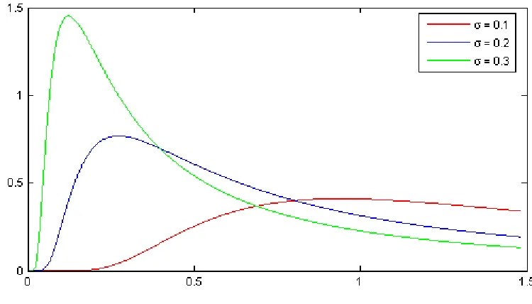
Letℎ(𝑡), where 0≤𝑡≤𝑇, denote the density of the ﬁrst exit time ie. the ﬁrst time 𝑡for which 𝑆𝑡=𝐵. See

Figure5.1. The required valuation is then 𝑉 =𝑒−𝑟𝑇∫𝑇

0 ℎ(𝑡)𝑑𝑡.

We first need to find the function ℎ(𝑡), and then perform the integration. We first suppose that𝐵 > 𝑆; the case where𝐵 < 𝑆 is similar but has some subtle differences. We proceed cautiously!

Hitting time for Brownian motion without drift (hit is high)

We ﬁrst establish the hitting time distribution for Brownian motion without drift. The ﬁrst hitting or stopping time is

𝜏= inf

𝑡≥0{𝑋(𝑡) =𝑏}

We suppose that 𝑏 >0. We can apply the optional sampling theorem to the stochastic integral because this stopped Brownian motion𝑋(𝑡∧𝜏) is bounded from above (but not below), and so𝑒𝜃𝑋(𝑡∧𝜏)−

1

2𝜃2(𝑡∧𝜏)_{is bounded}

from above by𝑒𝜃𝑏, and below by 0. Thus_𝔼

[ 𝑒𝜃𝑏−12𝜃

2_𝜏]

= 1 for any𝜃 >0.

Let𝑝𝑏 be the hitting time distribution. Letℒ denote the Laplace transformation. Then

ℒ[𝑝𝑏](𝑠) =

∫ ∞

0

𝑒−𝑠𝑡𝑝𝑏(𝑡)𝑑𝑡

=_𝔼[ 𝑒−𝑠𝜏]

=𝔼

[ 𝑒−

√

2𝑠𝑏+√2𝑠𝑏−𝑠𝜏]

=𝑒− √

2𝑠𝑏

𝔼

[ 𝑒

√ 2𝑠𝑏−𝑠𝜏]

=𝑒− √

2𝑠𝑏

by putting𝜃=√2𝑠. Thus

𝑝𝑏(𝑡) =ℒ−1[𝑒−

√

2𝑠𝑏_] _(5.7)

= 𝑏

𝑡3/2√₂_𝜋exp [

−1 2

𝑏2 𝑡

]

(5.8)

using [Abramowitz and Stegun,1974, 29.3.82].

Hitting time for Brownian motion with drift (hit is high)

Now let the ﬁrst hitting time be deﬁned as inf𝑡≥0{𝛼𝑡+𝑋(𝑡) =𝑏}. Here𝑋 is as before, the drift is𝛼 >0, and

the hit level we seek is𝑏 >0.

This time𝑋𝑏is the Brownian motion which is stopped when𝛼𝑡+𝑋(𝑡) ﬁrst hits𝑏. Again,𝑋𝑏 is bounded from

above by𝑏(we use the fact that 𝛼 >0).

We have seen the idea already: 𝔼[𝑒−𝑠𝜏] =𝔼[𝑒−𝜃𝑏+𝜃𝑏−𝑠𝜏]=𝑒−𝜃𝑏𝔼[𝑒𝜃𝑏−𝑠𝜏]=𝑒−𝜃𝑏, as𝔼[𝑒𝜃𝑏−𝑠𝜏]= 1, for some

cute choice of𝜃. This time,

𝜃𝑏−𝑠𝜏=𝜃[𝛼𝜏+𝑋𝑏(𝜏)]−𝑠𝜏

(26)

and so we should choose𝑠−𝜃𝛼= 1 2𝜃

2_{. Solving for}_{𝜃 >}_{0 yields}√₂_𝑠₊_𝛼2₋_𝛼_{. Again let}_𝑝

𝑏be the hitting time

distribution. Then

ℒ[𝑝𝑏](𝑠) =

∫ ∞

0

𝑒−𝑠𝑡𝑝𝑏(𝑡)𝑑𝑡

=𝔼[𝑒−𝑠𝜏]

=𝔼

[ 𝑒(𝛼−

√

2𝑠+𝛼2₎_𝑏₊₍√₂_𝑠₊_𝛼2₋_𝛼₎_𝑏₋_𝑠𝜏]

=𝑒(𝛼− √

2𝑠+𝛼2₎_𝑏

𝔼

[ 𝑒(

√

2𝑠+𝛼2₋_𝛼₎_𝑏₋_𝑠𝜏]

=𝑒(𝛼− √

2𝑠+𝛼2₎_𝑏

(5.9)

Thus

𝑝𝑏(𝑡) =ℒ−1[𝑒(𝛼−

√ 2𝑠+𝛼2₎_𝑏

] =𝑒𝛼𝑏ℒ−1_[_𝑒−√2𝑠+𝛼2_𝑏

]

=𝑒𝛼𝑏 𝑏

𝑡3/2√₂_𝜋exp [ −1 2 𝑏2 𝑡 ] 𝑒− 1 2𝛼2𝑡

= 𝑏

𝑡3/2√₂_𝜋exp [

−1 2

(_𝑏₋_𝛼𝑡

√

𝑡 )2]

(5.10)

using the previous Laplace transform result and [Abramowitz and Stegun, 1974, 29.2.12].

Hitting time for the stock price(𝐵 > 𝑆)

We are looking for the ﬁrst𝜏 satisfying𝑆𝑒𝑚−𝜏+𝜎𝑋(𝜏)₌_𝐵_{, so} _𝜏 _{is given by}

inf

{

𝑡≥0 : 𝑚−

𝜎 𝑡+𝑋(𝑡) =

1

𝜎ln 𝐵 𝑆

}

Making the substitution𝛼= 𝑚−

𝜎 ,𝑏=

1

𝜎ln 𝐵

𝑆 >0 we have the distribution of this hitting time in (5.10), which

we have agreed to nameℎ(𝑡): thus

ℎ(𝑡) = ln

𝐵 𝑆

𝜎𝑡3/2√₂_𝜋exp ⎡

⎣−1₂ (

ln𝐵 𝑆 −𝑚−𝑡

𝜎√𝑡

)2⎤

⎦ (5.11)

Now, remember if at all possible what we are doing here: we have𝑉 =𝑒−𝑟𝑇∫𝑇

0 ℎ(𝑡)𝑑𝑡. This is

𝑉up = 𝑒 −𝑟𝑇 ⎡ ⎣ (_𝐵 𝑆 )

2𝑚−

𝜎2

𝑁(𝑒+(𝑇)) +𝑁(−𝑒−(𝑇)) ⎤

⎦ (5.12)

𝑒±(𝑡) =

±ln𝑆 𝐵 −𝑚−𝑡

(27)

[image:27.612.124.499.129.343.2]

Figure 5.1: First exit time density

To show this, we establish in order the following identities:

𝑒−(𝑡)−𝑒+(𝑡) =

2

𝜎√𝑡ln 𝐵

𝑆 (5.14)

𝑒2₋=𝑒2₊−4𝑚−

𝜎2 ln 𝐵

𝑆 (5.15)

𝑁′(𝑒−) =𝑁′(𝑒+) (_𝐵

𝑆 )

2𝑚−

𝜎2

(5.16)

∂

∂𝑡𝑒±(𝑡) =

1

2𝑡𝑒∓(𝑡) (5.17)

𝑒±(0) =∓∞ (5.18)

ℎ(𝑡) = 𝑑

𝑑𝑡 (

𝐵 𝑆

) 2𝑚−

𝜎2

𝑁(𝑒+(𝑡))−𝑁(𝑒−(𝑡)) (5.19)

What if 𝐵 < 𝑆?

The diﬀerences appear already at the ﬁrst stage! This time𝑋𝑏 is bounded from below (but not above). The

Martingale we must consider is −√2𝑠𝑋𝑏(𝑡), and it then follows that𝔼

[ 𝑒−

√

2𝑠𝑏−𝑠𝜏]_{= 1. It then follows that}

ℒ[𝑝(𝑏, 𝑡)] =𝑒 √

2𝑠𝑏_.

One generalises each calculation in turn with the appropriate care. The value of the option is

𝑉down=𝑒−𝑟𝑇 ⎡

⎣ (

𝐵 𝑆

) 2𝑚−

𝜎2

𝑁(−𝑒+(𝑇)) +𝑁(𝑒−(𝑇))

⎤

(28)

5.3.3 No hit rebate

Clearly the value of the no-hit rebate is given by𝑒−𝑟𝑇₋_𝑉_{, because the sum of a hit rebate and a no-hit rebate}

is cash. This is an example of in-out parity.

5.3.4 American digital options

Wystup[2002]. Now the payoﬀ occurs as soon as the hit occurs, and the value is∫𝑇 0 𝑒

−𝑟𝑡_ℎ₍_𝑡₎_𝑑𝑡_.

By ﬁrst completing the square, and then following the same basic strategy as before, this value can be shown to be

𝑉𝜂=

(_𝐵

𝑆 )

𝑚−+𝑛−

𝜎2

𝑁(−𝜂𝑒+(𝑇)) +

(_𝐵

𝑆 )

𝑚− −𝑛−

𝜎2

𝑁(𝜂𝑒−(𝑇)) (5.21)

𝑛−= √

𝑚2

−+ 2𝜎2𝑟 (5.22)

𝑒±(𝑡) =

±ln_𝐵𝑆 −𝑛−𝑡

𝜎√𝑡 (5.23)

5.4 Exercises

1. Verify (5.6).

2. (exam 2003) Suppose we have a power option of term 𝜏. The payoﬀ of this option is (𝑆(𝑇)−𝐾)2 _if 𝑆(𝑇)> 𝐾, 0 otherwise. Price such an option, giving all details.

(29)

Chapter 6

Variance swaps

6.1 Contractual details

A long party in a variance swap will receive realised variance, and pay ﬁxed. Realised variance is deﬁned as

Σ = 𝑑

𝑁

∑

𝑖=1 (

ln 𝑆𝑖

𝑆𝑖−1 )2

where𝑆0, 𝑆1, . . . , 𝑆𝑁 are the stock prices on contractually speciﬁed days𝑡0, 𝑡1, . . . , 𝑡𝑁, and𝑑is the number

of contractually speciﬁed trade days in the year (so, 252 or 250 or suchlike). The deﬁnition of log returns might or might not be adjusted for dividends.

Very often the payoﬀ to a variance swap will be capped. The default seems to be at a cap level which corresponds to 2.5𝐾, where𝐾 is the strike in volatility terms. As such, these caps are irrelevant (worthless) in the case of index variance swaps. They may have relevance in the pricing of single equity variance swaps. Note that a position in a capped swap is the same as a position in a swap and a short position in a call. Thus, we restrict attention to the the case where there is no cap.

6.2 The theoretical pricing model

Here we followDemeterﬁ et al.[March 1999].

In a diﬀusion model, the realized variance for a given evolution of the stock price is the integral

Σ = 1

𝑇 ∫ 𝑇

0

𝜎2(𝑡)𝑑𝑡 (6.1)

This is a good approximation to the contractually deﬁned variance above.

The value of the pay ﬁxed leg of the variance swap with volatility strike𝐾is the expected present value of the payoﬀ in the risk-neutral world

𝑉 =𝑒−𝑟𝑇_𝔼ℚ[

Σ−𝐾2] (6.2)

(30)

Then

𝑑𝑆

𝑆 = (𝑟−𝑞)𝑑𝑡+𝜎(𝑡)𝑑𝑍 𝑑ln𝑆 =(𝑟−𝑞−1

2𝜎 2

(𝑡)) 𝑑𝑡+𝜎(𝑡)𝑑𝑍

so taking diﬀerences and rearranging we get

𝜎2(𝑡)𝑑𝑡= 2

(_𝑑𝑆

𝑆 −𝑑ln𝑆 )

Writing this in the integral form we have

∫ 𝑇 0

𝜎2(𝑡)𝑑𝑡= 2

∫ 𝑇 0

𝑑𝑆 𝑆 −2 ln

𝑆(𝑇)

𝑆(0)

Now𝔼ℚ

[_∫_𝑇 0

𝑑𝑆 𝑆

]

= (𝑟−𝑞)𝑇 - this is dynamically replicated by trading in futures - so the only problem is the log contract. In fact the log contract can theoretically be replicated using a continuum of option positions. Let𝑆∗ be some ﬁxed point. We decide what this means and what it should be in due course. Firstly, deﬁne

another exotic payoﬀ𝑓 by

𝑓(𝑆(𝑇)) :=𝑆(𝑇)−𝑆∗

𝑆∗ −ln 𝑆(𝑇)

𝑆∗ (6.3)

Thus

𝔼ℚ[Σ] =

2 𝑇𝔼 ℚ [ ∫ 𝑇 0 𝑑𝑆

𝑆 −ln 𝑆(𝑇)

𝑆(0)

]

= 2(𝑟−𝑞)− 2

𝑇𝔼 ℚ

[

ln𝑆(𝑇)

𝑆(0)

]

= 2(𝑟−𝑞)− 2

𝑇𝔼 ℚ

[_𝑆₍_𝑇₎₋_𝑆 ∗

𝑆∗ −𝑓(𝑆(𝑇)) + ln 𝑆∗ 𝑆(0)

]

= 2(𝑟−𝑞)− 2

𝑇

[_𝑆₍₀₎_𝑒(𝑟−𝑞)𝑇 ₋_𝑆

∗ 𝑆∗

−𝔼ℚ[𝑓(𝑆(𝑇))] + ln 𝑆∗

𝑆(0)

]

But now, we discover the remarkable

𝑓(𝑆(𝑇)) =

∫ 𝑆∗ 0

1

𝐾2max(𝐾−𝑆(𝑇),0)𝑑𝐾+ ∫ ∞

𝑆∗

1

𝐾2max(𝑆(𝑇)−𝐾,0)𝑑𝐾 (6.4)

and so

𝔼ℚ[Σ]

= 2(𝑟−𝑞)− 2

𝑇

𝑆(0)𝑒(𝑟−𝑞)𝑇 ₋_𝑆

∗ 𝑆∗

+2𝑒

𝑟𝑇

𝑇 [

∫ 𝑆∗ 0

1

𝐾2𝑝(𝐾)𝑑𝐾+ ∫ ∞

𝑆∗

1

𝐾2𝑐(𝐾)𝑑𝐾 ]

− 2

𝑇 ln 𝑆∗

𝑆(0) (6.5) We thus replicate 𝑓 by trading a continuum of puts with strikes from 0 to 𝑆∗ and a continuum of calls with

strikes from 𝑆∗ to ∞. The weight of the options in the continuum is proportional to _𝐾12. So, this clearly

motivates us to choose𝑆∗ to be a point below which we prefer to use puts, and above which we prefer to use calls for replication. In this we prefer to use out-the-money options at all times, because they are more liquid than in-the-money options. So 𝑆∗ might be the liquid strike on the skew closest to the forward level of𝑆, for example.

(31)

6.3 Super-replication

The only diﬃculty is that to replicate we require a continuum of options. In reality of course this is impossible. Thus we seek a super-replication strategy.

Of course it is the payoﬀ of𝑓 that needs to be super-replicated, everything else can be done straightforwardly. On the region [𝐾1, 𝐾𝑚] we can super-replicate the payoﬀ 𝑓 with a portfolio of options: exactly those options

used to calculate the theoretical variance.

For the region [𝐾𝑛, 𝐾𝑚] we choose the following calls:

• 𝑓(𝐾𝑛+1)−𝑓(𝐾𝑛)

𝐾𝑛+1−𝐾𝑛 many calls struck at 𝐾𝑛, plus

• 𝑓(𝐾𝑗+1)−𝑓(𝐾𝑗)

𝐾𝑗+1−𝐾𝑗 −

𝑓(𝐾𝑗)−𝑓(𝐾𝑗−1)

𝐾𝑗−𝐾𝑗−1 many calls stuck at 𝐾𝑗 for𝑗 =𝑛+ 1, . . . , 𝑚−1.

This super-replicates in the region [𝐾𝑛, 𝐾𝑚] and sub-replicates in the region [𝐾𝑚,∞). We choose in addition

• 𝑓′(𝐾𝑚)−

𝑓(𝐾𝑚)−𝑓(𝐾𝑚−1)

𝐾𝑚−𝐾𝑚−1 many calls struck at𝐾𝑚.

which improves things in the region [𝐾𝑚,∞). Note that super-replication in that region is impossible.

For the region [𝐾1, 𝐾𝑛] we choose the following puts:

• 𝑓(𝐾𝑛−1)−𝑓(𝐾𝑛)

𝐾𝑛−𝐾𝑛−1 many puts struck at𝐾𝑛, plus

• 𝑓(𝐾𝑗−1)−𝑓(𝐾𝑗)

𝐾𝑗−𝐾𝑗−1 −

𝑓(𝐾𝑗)−𝑓(𝐾𝑗+1)

𝐾𝑗+1−𝐾𝑗 many puts struck at𝐾𝑗 for𝑗=𝑛−1, . . . , 2.

This super-replicates in the region [𝐾1, 𝐾𝑛] and sub-replicates in the region [0, 𝐾1]. We choose in addition

• −𝑓′(𝐾1)−𝑓(𝐾1)−𝑓(𝐾2)

𝐾2−𝐾1 many puts struck at𝐾1.

which improves things in the region [0, 𝐾1]. Note that super-replication in that region is impossible.

6.4 Exercises

1. What is the price of an oﬀ-the-run variance swap i.e. one that has already started? Write it as a function of history and the price of a just starting variance swap.

2. The notional of the variance swap is usually quoted in ‘vega notional’𝒱𝑁, where the vega notional and

the cash (variance) notional $𝑁 are related by $𝑁 = 𝒱₂_𝐾𝑁. Show that with this deﬁnition, if the realised

(32)

Chapter 7

Compound options

A compound option is an option in which the underlying is an option. Thus, there is a ﬁrst exercise date, and if exercised, a vanilla option is born, for a (necessarily subsequent) exercise date.

The following analysis is based on the work of Geske Geske [1979b] who investigated equity options and hypothesised that an equity itself behaved like an option. Geske’s model used the assumptions of the Black-Scholes model: constant volatility, constant interest rates, no dividend yield, no transaction costs etc. Logical adjustments to Geske’s model allow the three term structures of volatility, interest rates and dividend yields to be reﬂected in the premium.

𝑇2 ∼ maturity of underlying option.

𝑇1 ∼ maturity of compound option,𝑇1≤𝑇2. 𝑡 ∼ valuation date of the compound option.

𝜏2 = 𝑇2−𝑇1, in years.

𝜏1 = 𝑇1−𝑡, in years.

𝜏 = 𝑇2−𝑡, in years.

𝐾2 ∼ strike of underlying option.

𝐾1 ∼ strike of compound option.

𝑟 ∼ risk free rate

𝜎 ∼ volatility

𝑞 ∼ expected dividend yield

𝑆𝑡 ∼ spot of underlying stock at time 𝑡.

(33)

are all similar. Let BS(𝑦) be the value of the underlying option at time𝑇1 that corresponds to𝑆(𝑦). Thus

𝑆(𝑦) = 𝑆𝑒𝑚−𝜏1+𝜎 √

𝜏1𝑦 _(7.1)

BS(𝑦) = 𝑆(𝑦)𝑒−𝑞𝜏2_𝑁₍_𝑑+₎₋_𝐾2𝑒−𝑟𝜏2_𝑁₍_𝑑

−) (7.2)

𝑑± =

ln𝑆_𝐾(𝑦)

2 +𝑚±𝜏2 𝜎√𝜏2

= ln

𝑆

𝐾2 +𝑚−𝜏1+𝑚±𝜏2+𝜎

√

𝜏1𝑦

𝜎√𝜏2

= ln

𝑆

𝐾2 +𝑚−𝜏1+𝑚±𝜏2 𝜎√𝜏2

+

√_𝜏1

𝜏2

𝑦 (7.3)

Let𝑦∗ be such that BS(𝑦∗) =𝐾1. 𝑦∗is found using Newton’s method, with

𝑦0 = 0 𝑦𝑛+1 = 𝑦𝑛−

BS(𝑦𝑛)−𝐾1

∂

∂𝑦BS(𝑦)∣𝑦𝑛

Then

𝑉 = 𝑒−𝑟𝜏1 ∫ ∞

𝑦=−∞

[BS(𝑦)−𝐾1]+𝑁′(𝑦)𝑑𝑦

= 𝑒−𝑟𝜏1 ∫ ∞

𝑦=𝑦∗

(BS(𝑦)−𝐾1)𝑁′(𝑦)𝑑𝑦

= 𝑒−𝑟𝜏1 ∫ ∞

𝑦=𝑦∗

(𝑆(𝑦)𝑒−𝑞𝜏2_𝑁₍_𝑑+₎₋_𝐾2𝑒−𝑟𝜏2_𝑁₍_𝑑

−)−𝐾1)𝑁′(𝑦)𝑑𝑦

= 𝑒−𝑟𝜏1_𝑆𝑒𝑚−𝜏1_𝑒−𝑞𝜏2 ∫ ∞

𝑦=𝑦∗ 𝑒𝜎

√

𝜏1𝑦_𝑁₍_𝑑+₎_𝑁′₍_𝑦₎_𝑑𝑦 _(7.4)

−𝑒−𝑟𝜏1_𝐾 2𝑒−𝑟𝜏2

∫ ∞

𝑦=𝑦∗

𝑁(𝑑−)𝑁′(𝑦)𝑑𝑦 (7.5)

−𝑒−𝑟𝜏1_𝐾 1

∫ ∞

𝑦=𝑦∗

𝑁′(𝑦)𝑑𝑦 (7.6)

(7.4) follows from a careful application of (1.19), and (7.5) follows from a careful application of (1.18). Of course (7.6) is trivial.

Let𝜂=±1 if the underlying option is a call/put and𝜁=±1 if the compound option is a call/put. Then the value of the compound option is

𝑉 = 𝜂𝜁𝑆𝑒−𝑞𝜏𝑁2 (

−𝜂𝜁(𝑦∗−𝜎

√

𝜏1), 𝜂𝑑+, 𝜁 √

𝜏1 𝜏

)

−𝜂𝜁𝐾2𝑒−𝑟𝜏𝑁2 (

−𝜂𝜁𝑦∗, 𝜂𝑑−, 𝜁 √

𝜏1 𝜏

)

−𝜁𝐾1𝑒−𝑟𝜏1𝑁(−𝜂𝜁𝑦∗) (7.7) 𝑑± = ln

𝑆

𝐾2 +𝑚±𝜏

𝜎√𝜏 (7.8)

7.1 Exercises

(34)

2. Fill in the missing details in the notes for getting the ﬁnal pricing formula for a compound call on call option.

3. (exam 2003) Suppose we wish to price a compound call on call, where all of risk free, dividend yield and volatility have a term structure. (There is however no skew structure to volatility.) Let the compound option expire after time𝜏1(in years) with strike 𝑋1 and let the relevant rates be𝑟1,𝑞1and𝜎1. Let the vanilla option expire after time𝜏2 (in years) with strike𝑋2 and let the relevant rates be𝑟2,𝑞2 and𝜎2.

(a) What are the forward rates for the period from𝜏1 to 𝜏2 in terms of the ordinary rates for𝜏1 and

𝜏2? Denote them henceforth as𝑟𝑓,𝑞𝑓 and𝜎𝑓,

(b) Now price such an option, following the following hints which come from the notes:

• Let𝑆(𝑦) be the value of the underlying and BS(𝑦) be the value of the underlying option at time

𝜏1if the draw from the 𝜙(0,1) distribution has been𝑦. Thus𝑆(𝑦) =....and BS(𝑦) =...

• Let 𝑦∗ be such that BS(𝑦∗) = 𝑋1. 𝑦∗ is found using Newton’s method, with .... (include the

diﬀerentiation).

• Then𝑉 =....

For the ﬁnal part, you may use without proof the following two facts

∫ ∞

𝛼

𝑁(𝐾+𝐿𝑥)𝑁′(𝑥)𝑑𝑥 = 𝑁2 (

−𝛼, √ 𝐾

𝐿2_{+ 1}, 𝐿

√

𝐿2_{+ 1} )

∫ ∞

𝛼

𝑒𝐴𝑥𝑁(𝐾+𝐿𝑥)𝑁′(𝑥)𝑑𝑥 = 𝑒𝐴 2 2 _𝑁2

(

−𝛼+𝐴, √𝐾+𝐴𝐿

𝐿2_{+ 1}, 𝐿

√

𝐿2_{+ 1} )

4. (exam 2008) This question concerns pricing a complex chooser option. Such an option is valued today

𝑡0; at time 𝑡1 the owner has to choose between owning

• A call with a maturity date𝑡𝐶 and strike𝐾𝐶;

• A put with a maturity date𝑡𝑃 and strike𝐾𝑃.

Volatility, dividend yield, and the risk free rate are all constant.

(a) I can write the value of 𝑆(𝑡1) as 𝑆(𝑡0)𝑒⋅⋅⋅𝑧 where 𝑧 is a random sample from a normal distribution with mean 0 and standard deviation 1. Complete the⋅ ⋅ ⋅ here.

(b) Hence write the value AT TIME𝑡1 of the call as a function BS𝐶(𝑧) and the value of the put as a function BS𝑃(𝑧), being careful to distinguish between𝑑𝐶

± for the call and𝑑𝑃± for the put.

(c) Explain why there will be a value of 𝑧, call it 𝑧∗, where we will be indiﬀerent to selecting the put or the call. A diagram might be useful. Say how𝑧∗ will be found, although you are not required to give any details.

(d) Write down the value of the option in terms of integrals.

(35)

Chapter 8

Basket Options

Suppose the assets have value weights 𝑤𝑖 in the basket, where ∑ 𝑛

𝑖=1𝑤𝑖 = 1. Suppose we have a covariance

matrix Σ. The basket volatility is then√𝑤′_Σ_𝑤_{. A European option on the basket can then be priced in the}

usual way with this volatility.

These are the forward weights rather than the valuation date weights. The forward weights will be diﬀerent to the spot weights because the dividend yields / discrete dividends are diﬀerent.

All analytic models make the assumption that the basket value is actually the geometric mean of the various underlyings rather than the arithmetic mean. This methodology was first proposed in Gentle[1993]. In fact, the above formulation of the basket volatility placed in the geometric Brownian motion framework is implicitly making this assumption. (This is a non-trivial point - see [Musiela and Rutkowski,1998,§9.9] for an excellent discussion.) Academic and market research has shown however that the effect of this is not severe, especially considering that this assumption has remarkable computational advantages over a lattice methodology such as that of Rubinstein[1994] - this approach will choke on any basket which has many underlyings - even three underlyings will make the calculation slow. An alternative is to work out the first few (even the first two) moments of the arithmetic basket and then fit an analytically tractible distribution to these moments. We will see this applied in the setting of Asian options. Of course, we could use this geometric basket price as a control variate when doing Monte Carlo.

Here is the solution of Gentle [1993]. Suppose the option is on the basket ∑𝑛

𝑖=1𝑊𝑖𝑆𝑖, where as usual

𝑊1, 𝑊2, . . . , 𝑊𝑛 are the number of each of the shares in the basket. First note that

𝑉(0) =𝑒−𝑟𝜏𝔼

[

max

( 𝜂

( 𝑛

∑

𝑖=1

𝑊𝑖𝑆𝑖(𝑇)−𝐾

) ,0

)]

=𝑒−𝑟𝜏𝔼

[

max

( 𝜂

( 𝑛

∑

𝑖=1

𝑤𝑖𝑆𝑖∗(𝑇)−𝐾

∗ )

,0

)] 𝑛

∑

𝑖=1 𝑊𝑖𝑓𝑖

where𝑤𝑖=

𝑊𝑖𝑓𝑖

∑𝑛 𝑗=1𝑊𝑗𝑓𝑗 𝑆_𝑖∗(𝑇) = 𝑆𝑖(𝑇)

𝑓𝑖

𝐾∗= _∑𝑛𝐾 𝑖=1𝑊𝑖𝑓𝑖

Now ∑𝑛

𝑖=1𝑤𝑖𝑆𝑖∗(𝑇) is a weighted arithmetic average of numbers𝑆𝑖∗(𝑇) with expectations all equal to 1. We

(36)

expected diﬀerence. Put

𝑌 :=

𝑛

∏

𝑖=1

(𝑆_𝑖∗(𝑇))𝑤𝑖

𝛼:= exp

⎛ ⎝− 𝜏 2 𝑛 ∑ 𝑗=1 𝑤𝑗𝜎𝑗2

⎞

⎠

and so ln𝑌 ∼𝜙(ln𝛼,√𝑤′_Σ_𝑤√_𝜏)_{. Then}

𝑉(0) =𝑒−𝑟𝜏𝔼

[ max ( 𝜂 ( 𝑛 ∑ 𝑖=1

𝑤𝑖𝑆𝑖∗(𝑇)−𝐾

∗ ) ,0 )] 𝑛 ∑ 𝑖=1 𝑊𝑖𝑓𝑖

=𝑒−𝑟𝜏_𝔼 [ max ( 𝜂 ( 𝑌 + 𝑛 ∑ 𝑖=1

𝑤𝑖𝑆𝑖∗(𝑇)−𝑌 −𝐾

∗ ) ,0 )] _𝑛 ∑ 𝑖=1 𝑊𝑖𝑓𝑖

≈𝑒−𝑟𝜏𝔼

[

max(𝜂(𝑌 + 1−𝛼𝑒1/2𝑤′Σ𝑤𝜏−𝐾∗),0)]

𝑛

∑

=𝑒−𝑟𝜏𝔼[max(𝜂(𝑌 −𝐾),0)]

𝑛

∑

where −𝐾= 1−𝛼𝑒1/2𝑤′Σ𝑤𝜏−𝐾∗

Now, using Lemma3.3.1and after some tedious manipulations, we have

𝑉(0)≈𝜂𝑒−𝑟𝜏[ ˜𝑓 𝑁(𝜂𝑑+)−𝐾𝑁˜ (𝜂𝑑−)] (8.1) ˜

𝑓 =

𝑛

∑

𝑖=1

𝑊𝑖𝑓𝑖𝛼𝑒1/2𝑤

′_Σ_𝑤𝑇

(8.2)

˜

𝐾=𝐾+

𝑛

∑

𝑖=1

𝑊𝑖𝑓𝑖(𝛼𝑒1/2𝑤

′_Σ_𝑤𝑇

−1) (8.3)

𝑑±=

ln 𝑓_˜˜

𝐾 ±

1 2

√

𝑤′_Σ_𝑤2_𝜏

√

(37)

Chapter 9

Rainbow options

A version of this chapter appears inOuwehand and West [2006].

9.1 Deﬁnition of a Rainbow Option

Rainbow Options refer to all options whose payoﬀ depends on more than one underlying risky asset; each asset is referred to as a colour of the rainbow. Examples of these include:

• “Best of assets or cash” option, delivering the maximum of two risky assets and cash at expiry Stulz

[1982], Johnson[1987],Rubinstein[1991]

• “Call on max” option, giving the holder the right to purchase the maximum asset at the strike price at expriryStulz[1982],Johnson [1987]

• “Call on min” option, giving the holder the right to purchase the minimum asset at the strike price at expiryStulz[1982], Johnson[1987]

• “Put on max” option, giving the holder the right to sell the maximum of the risky assets at the strike price at expiry, Margrabe[1978],Stulz[1982],Johnson[1987]

• “Put on min” option, giving the holder the right to sell the minimum of the risky assets at the strike at expiryStulz[1982], Johnson[1987]

• “Put 2 and call 1”, an exchange option to put a predeﬁned risky asset and call the other risky asset,

Margrabe [1978]. Thus, asset 1 is called with the ‘strike’ being asset 2.

Thus, the payoﬀs at expiry for rainbow European options are: Best of assets or cash max(𝑆1, 𝑆2, . . . , 𝑆𝑛, 𝐾)

Call on max max(max(𝑆1, 𝑆2, . . . , 𝑆𝑛)−𝐾,0)

Call on min max(min(𝑆1, 𝑆2, . . . , 𝑆𝑛)−𝐾,0)

Put on max max(𝐾−max(𝑆1, 𝑆2, . . . , 𝑆𝑛),0)

Put on min max(𝐾−min(𝑆1, 𝑆2, . . . , 𝑆𝑛),0)

Put 2 and Call 1 max(𝑆1−𝑆2,0)

Exotic equity options