AI KU at SemEval 2016 Task 11: Word Embeddings and Substring Features for Complex Word Identification

AI-KU at SemEval-2016 Task 11: Word Embeddings and Substring

Features for Complex Word Identification

Onur Kuru

Artificial Intelligence Laboratory Koc University

Istanbul, Turkey

[email protected]

Abstract

We investigate the usage of word embeddings, namely Glove and SCODE, along with sub-string features on Complex Word Identifica-tion task. We introduce two systems: the first system utilizes the word embeddings of the target word and its substrings as features while the other considers the context infor-mation by using the embeddings of the sur-rounding words as well. Although the pro-posed representations perform below the aver-age with nonlinear models, we show that word embeddings with substring features is an ef-fective representation choice when employed with linear classifiers.

1 Introduction

Complex Word Identification (CWI) is the task of determining which words in a given sentence should be simplified. CWI is often considered as the first step in Lexical Simplification (LS) where the goal is to identify and replace complex words with sim-pler substitutes. Although CWI is considered as a vital component of Lexical Simplification pipeline, there is not a lot of work done for identifying word complexity in the context of Lexical Simplification. Horn et al. (2014) describes an LS model in which they employ a Complex Word identifier implicitly. However, their results show that the method is not able to capture complex words very accurately.

Paetzold and Specia (2016) organizes the Com-plex Word Identification task of SemEval 2016 with the goal of attracting systems that are able to de-tect complex words in given a sentence. This work

investigates the usage of word embeddings along with substrings as features to build a Complex Word Identifier. Word embeddings are unsupervised word representations which map each word to a dense, real valued, low dimensional vector. These vectors are able to capture semantic and syntactic similar-ities between words and proven useful as features in a variety of applications, such as, document clas-sification (Sebastiani, 2002), named entity recogni-tion (Turian et al., 2010), and parsing (Socher et al., 2013).

GloVe (Pennington et al., 2014) is an unsuper-vised learning algorithm for obtaining vector rep-resentations for words which is essentially a log-bilinear model with a weighted least-squares ob-jective. Pennington et al. (2014) shows that the word embeddings produced by the model achieves state-of-the-art performance in Word Analogy task. Moreover, they also illustrate that Glove embed-dings outperform embedembed-dings induced by other methods on several word similarity tasks.

Another work (Yatbaz et al., 2012) represents the context of a word by its probable substitutes. Words with their probable substitutes are fed to a co-occurrence modeling framework (SCODE) (Maron et al., 2010). Words co-occurring in similar context are closely embedded on a sphere. These word em-beddings are effective at modeling syntactic features and they achieve state-of-the-art results in inducing part-of-speech.

We conducted several experiments to examine the usage of word embeddings. First, we investigated whether pretrained word embeddings improve ran-dom embedding baseline. Second, we tried

nations of word embeddings with different types and dimensions. Next, we examined context-aware rep-resentations of target words by incorporating em-beddings of neighbouring words. After the release of test set annotations, we scrutinize how a linear model benefits from increasing the size of the train-ing set.

This paper is organized as follows: Section 2 details the proposed dataset and evaluation metric, Section 3 analyzes the utilization of word embed-dings for CWI, Section 4 presents results and dis-cusses the performance of our work and Section 5 concludes the paper.

2 Dataset and Evaluation

Complex Word Identification task of SemEval 2016 (Paetzold and Specia, 2016) prepares a dataset with 200 sentences for training and 9000 for testing. The training set is composed of 5,362 tokens with 2,237 instances annotated, and the test set is composed of 217,902 tokens with 88,221 instances annotated. Dataset properties are summarized in Table 1.

9,200 sentences were annotated through a survey, in which 400 volunteers were presented with sev-eral sentences and asked to judge whether or not they could understand the meaning of each word in a given sentence. A set of 200 sentences is sepa-rated for training and split into 20 subsets of 10 sen-tences, and each subset was annotated by a total of 20 volunteers. In the training set, a word is consid-ered as complex if at least one of the 20 annotators judged them so. To compose the test set, remain-ing 9,000 sentences were split into 300 subsets of 30 sentences, each of which was annotated by a single volunteer.

Training Test Annotated 2237 88221 Tokens 5362 217902 Sentences 200 9000

Table 1:Dataset Properties

Notably, training set is extremely small compared to test set. As a result of this, 92% of test set vocab-ulary is unknown to training set.

In the context of Lexical Simplification, a CW identifier is expected to accomplish two things. First, it should predict the complexity of words

as proficiently as possible (Accuracy). Second, it should capture as many of the complex words as possible (Recall) to maximize the simplicity of a sentence. Therefore, instead of F-Score (harmonic mean of Precision and Recall), CWI task defines and uses G-Score which measures the harmonic mean between Accuracy and Recall.

3 Experiments 3.1 Word Embeddings

To illustrate the effect of word embeddings on CWI task, we conducted several experiments. For Glove word embeddings, we used the publicly avail-able word vectors1_{pretrained on a 2014 Wikipedia}

dump2 _{with 1.6 billion tokens merged with}

Giga-word 5 which has 4.3 billion tokens. We use a sample from Wikipedia dump with approximately 150 million tokens to induce SCODE word em-beddings3_{. For each word embedding experiment,}

we used Support Vector Machines with linear ker-nel as our classifier. We utilized scikit-learn (Buit-inck et al., 2013) as our machine learning arsenal. We applied 5-fold cross validation on training set and report the result at the optimum C (penalty pa-rameter of the error term) from a grid search in e−20_{, e}−19_{, ..., e}6_{, e}7_.

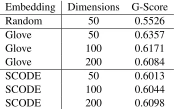
Embedding Dimensions G-Score

Random 50 0.5526

Glove 50 0.6357

Glove 100 0.6171

Glove 200 0.6084

SCODE 50 0.6013

SCODE 100 0.6044

SCODE 200 0.6098

Table 2:Random Embedding Baseline, Comparison of Glove and SCODE.

Firstly, each annotated word in a sentence repre-sented with its corresponding dense real valued em-bedding and fed to the classifier. As a simple base-line we assigned a random embedding to each an-notated word. A random embedding consists of 50 dimensions and each component is drawn from uni-form distributionU(0,1). Table 2 holds the results

for each experiment. We observe that both SCODE and Glove outperforms the random embedding base-line and Glove (trained on a much generous corpus) yields better results in general. Increasing the num-ber of dimensions improves the performance slightly for SCODE but it hurts the performance of Glove embeddings.

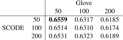
Glove

50 100 200

50 0.6559 0.6317 0.6185 SCODE 100 0.6514 0.6310 0.6174 200 0.6531 0.6323 0.6189 Table 3:Embedding Concatenations.

Subsequently, we took the cartesian product of both embeddings and experimented with concatena-tions. Instead of representing a word with only one embedding, we employed the concatenation of em-beddings as features for each target word. Results are presented in Table 3. Experiments yield the best results when we use 50 dimensional embeddings of both methods. We show that concatenating embed-dings yields better results.

k=0 k=1 k=2 k=3

S-50 G-50 0.6559 0.6393 0.6260 0.6206 S-100 G-50 0.6514 0.6394 0.6260 0.6204 S-200 G-50 0.6531 0.6399 0.6264 0.6207 Table 4: Context-Aware Representations. S and G denotes SCODE and Glove respectively. k is the number of left and right neighbors.

Moreover, we took the surrounding words into ac-count to make the representation of a target word context-aware. In this setup, each target word is rep-resented not only by its own embedding but also with embeddings of surrounding words. As can-didates, we selected the best performing concate-nated embeddings from Table 3. Table 4 lists the results for context-aware representations wherekis the number of left and right neighbors. Results im-ply that context-aware representations do not yield any improvements.

3.2 Final System

We submitted two systems4 _{for the Complex Word}

Identification task. Both systems use SVM classifier

4_{Code is available at: https://github.com/kuruonur1/cwi}

trained with Radial Basis Function. While first system (native) use the word embedding of the target word and its substrings as features, the second system (native1) uses the embeddings of preceding and following words as well. For target and surrounding words, we used the concatenation of SCODE and Glove with 50 dimensions which performed best for word embedding experiments. As substring features of the target word, we used prefixes, suffixes and character n-grams which are of length 3 and 4. We applied chi-squared test between each substring feature and class to reveal which ones are more relevant to classification and we kept theppercentile of highest scoring substring features.

C γ p G-Score

native 0.2705 0.1370 17 0.6800 native1 0.0595 0.0251 20 0.6500 Table 5:Best performed hyperparameters and 5-fold cross val-idation results on training set.Cis the penalty parameter of the error term for SVM,γis the coefficient of RBF kernel. p de-notes the percentile of substrings utilized with feature selection.

Either system has 3 parameters: the coefficient of RBF kernel (γ), penalty parameter of the error term (C), percentile(p)of substring features. In

or-der to tune the hyperparameters, we ran a random search (Bergstra and Bengio, 2012) using Hyper-opt (Bergstra et al., 2013). For each hyperparameter configuration, we drawnC andγ fromeU(−15,5)_,p fromU(5,30). For each system, we tried 100

hyper-parameter configurations and applied 5-fold cross validation. We selected the best performed hyperpa-rameters (see Table 5) and trained our final models on the whole training set.

4 Results and Discussion

base-line is released before system results and classifies a word as complex only if it is not in the Ogdens vo-cabulary5_{. We present our final systems’ results on}

test set with baselines scores in Table 6. Best Result6 _0.7740

nativeLin7 _0.7328

(TB) Wikipedia 0.6720 (TB) Simple Wiki 0.6540 (TB) Senses 0.5790

native1 0.5450

native 0.5450

(TB) Length 0.4780 (LB) Ogdens 0.3930

Table 6:Final system results on test set along with baselines

First and foremost, we see that both of our submit-ted systems perform equally well on test set. There-fore, taking the surrounding words into account does not yield any improvements as we observed while validating our model on training set. Although the threshold-based baselines simply look at the fre-quency of a word in a corpus, they outperform our rather sophisticated systems significantly.

One may hypothesize that the small amount of training set available is the main cause of this un-satisfactory performance. After the release of anno-tated test set, we examined the effect of amount of training set available to our system.

# of sentences G-Score training set 0.7451

+200 0.7475 +400 0.7512 +800 0.7559 +1600 0.7588 +3200 0.7638 +6400 0.7670

Table 7: G-Scores on held out test set while number of sen-tences in training set increasing.

We held out 1000 sentences from test set as our new test set. We started with the original training set and added sentences from annotated test set. We used the same configuration asnativesystem except

5_{http://ogden.basic-english.org/words.html} 6_{Best scoring system on SemEval-2016 CWI task}

7_{This model is evaluated on test set after official results are}

announced

we used a linear kernel instead of nonlinear RBF kernel to speed up experiments. For each training set we cross validated the penalty parameter of the error term (C) and evaluated it on held out test set. For each experiment, we report the mean G-Score of 5 random runs where the extra training set and held out test set splits selected from different shuffles. Ta-ble 7 illustrates that as the amount of training set in-creases our model performs better on held-out test set. Another key observation is that albeit our sys-tem is trained on the original training set with linear kernel, it has a high G-Score. Moreover, all other participants of CWI task which utilize word embed-dings use nonlinear models. This scrutiny refutes the hypothesis that small amount of training set is the primary cause of word embeddings’ unsatisfactory performance. Finally we trainednativesystem with linear kernel using only the original training set and evaluated on whole test set. Native system with lin-ear kernel (nativeLin) achieves a G-Score of0.7328

on whole test set.

5 Conclusion

We investigated the utilization of word embeddings along with substrings as features on Complex Word Identification task. We showed that instead of rep-resenting a word with only one embedding type, word embedding concatenations yield better results. Moreover we considered context information by in-corporating the embeddings of surrounding words which did not improve overall performance. Al-though the proposed representations perform below the average with nonlinear models, we conclude that word embeddings with substring features is an ef-fective representation choice when employed with linear classifiers.

References

James Bergstra and Yoshua Bengio. 2012. Random search for hyper-parameter optimization. The Journal of Machine Learning Research, 13(1):281–305. James Bergstra, Daniel Yamins, and David Daniel Cox.

2013. Making a science of model search: Hyperpa-rameter optimization in hundreds of dimensions for vi-sion architectures.

Grobler, Robert Layton, Jake VanderPlas, Arnaud Joly, Brian Holt, and Ga¨el Varoquaux. 2013. API design for machine learning software: experiences from the scikit-learn project. InECML PKDD Workshop: Lan-guages for Data Mining and Machine Learning, pages 108–122.

Colby Horn, Cathryn Manduca, and David Kauchak. 2014. Learning a lexical simplifier using wikipedia. InACL (2), pages 458–463.

Yariv Maron, Elie Bienenstock, and Michael James. 2010. Sphere embedding: An application to part-of-speech induction. InAdvances in Neural Information Processing Systems, pages 1567–1575.

Gustavo H. Paetzold and Lucia Specia. 2016. Semeval 2016 task 11: Complex word identification. In Pro-ceedings of the 10th International Workshop on Se-mantic Evaluation (SemEval 2016).

Jeffrey Pennington, Richard Socher, and Christopher D Manning. 2014. Glove: Global vectors for word rep-resentation. InEMNLP, volume 14, pages 1532–1543. Fabrizio Sebastiani. 2002. Machine learning in auto-mated text categorization. ACM computing surveys (CSUR), 34(1):1–47.

Richard Socher, John Bauer, Christopher D Manning, and Andrew Y Ng. 2013. Parsing with compositional vec-tor grammars. InACL (1), pages 455–465.

Joseph Turian, Lev Ratinov, and Yoshua Bengio. 2010. Word representations: a simple and general method for semi-supervised learning. InProceedings of the 48th annual meeting of the association for computational linguistics, pages 384–394. Association for Computa-tional Linguistics.