Artificial Bee colony for resource constrained project scheduling problem Pages 45-60 Download PDF

(1)

* Corresponding author Tel +98-917-1003767 Fax +98-711-6271747. E-mail addresses: [email protected] (R. Akbari),

Contents lists available atGrowingScience

International Journal of Industrial Engineering Computations

homepage: www.GrowingScience.com/ijiec

Artificial Bee colony for resource constrained project scheduling problem

Reza Akbaria*, Vahid Zeighamib and Koorush Ziaratia

a_{Department of Computer Science and Engineering, Shiraz University, Shiraz, Iran} b _{Department of Mathematics , School of Science, Shiraz University, Shiraz, Iran}

A R T I C L E I N F O A B S T R A C T

Article history: Received 15 April 2010 Received in revised form 19 July 2010

Accepted 20 July 2010 Available online 20 July 2010

Solving resource constrained project scheduling problem (RCPSP) has important role in the context of project scheduling. Considering a single objective RCPSP, the goal is to find a schedule that minimizes the makespan. This is NP-hard problem (Blazewicz et al., 1983) and one may use meta-heuristics to obtain a global optimum solution or at least a near-optimal one. Recently, various meta-heuristics such as ACO, PSO, GA, SA etc have been applied on RCPSP. Bee algorithms are among most recently introduced meta-heuristics. This study aims at adapting artificial bee colony as an alternative and efficient optimization strategy for solving RCPSP and investigating its performance on the RCPSP. To evaluate the artificial bee colony, its performance is investigated against other meta-heuristics for solving case studies in the PSPLIB library. Simulation results show that the artificial bee colony presents an efficient way for solving resource constrained project scheduling problem.

Keywords: Meta-heuristic Artificial bee colony Resource constrained project scheduling

Makespan Single mode

1. Introduction

Resource constrained project scheduling is known as an important problem in project scheduling. The RCPSP is an optimization problem which tries to find the optimum ordering of the activities to achieve some predefined objectives. It is possible to have many different objectives such as makespan, robustness, etc which are depended on some predefined goals (Abbasi et al., 2006). The makespan minimization, which is referred to as finding the minimum time to complete the entire project, is the most common objective in RCPSP. Also, RCPSP has several varieties so-called single-mode RCPSP (Ranjbar, 2008), multi-single-mode RCPSP (Damak et al., 2009), RCPSP with non-regular objective functions (Neumann et al., 2003), stochastic RCPSP (Rabbani et al., 2007; Ashtiani et al., 2009), Bin-packing related RCPSP (Fekete & Schepers, 1998), and multi-RCPSP (Krüger & Scholl, 2009). These varieties of RCPSP along with different possible objectives provide a wide area of research. Hence, scheduling resource constrained project has been the subject of extensive researches in the recent years.

(2)

(2010). The proposed methods can be classified as exact, heuristics and meta-heuristics. Exact methods are the first class of RCPSP solvers. Several exact methods have been proposed by authors to solve the RCPSP. The methods proposed by Stork and Uetz (2005), Sprecher (2000), and Mingozzi et al. (1998) are among the most representative exact methods. Although exact methods provide efficiency to solve small-sized instances of the RCPSP, they may not able to solve large-size instances of the RCPSP in a reasonable computational time. Therefore, we need to use heuristics or meta-heuristics when solving large problem instances. These approaches provide optimal or near optimal solutions for the problem at hand. The second class of RCPSP solvers is designed based on heuristics. The methods presented by Tormos and Lova (2001), Kolisch (1996), and Boctor (1990) are examples of the heuristic approaches. The methods of this class start with an empty schedule (i.e. none of the activities has been scheduled). After that, the empty schedule is filled by selecting a subset of activities in each step and assigning the earliest possible starting times to these activities by considering the priority rules and scheduling scheme. This process is continued until all the activities have been considered.

In scheduling process, the activities are selected based on their ranks, and the priority rules are used for ranking the activities. Meta-heuristics are used to design the third class of RCPSP solvers. Several meta-heuristic methods such as Tabu-Search (TS) (Tomas & Salhi, 1998), Simulated Annealing (SA) (Boctor, 1996; Bouleimen & Lecocq, 1993), Genetic Algorithm (GA) (Valls et al., 2008; Mendes et al., 2009), Scatter Search (Mobini et al., 2009), Electromagnetism (EM) (Debels & Vanhoucke, 2004), Immune Algorithm (IA) (Mobini et al. , 2010), Filter and Fan (FF) (Ranjbar, 2008), and Particle Swarm Optimization (PSO) (Chen et al., 2010; Zhang et al., 2005; Zhang et al., 2006) have been proposed by authors. The meta-heuristics approaches can be divided in two main sub-classes. The first sub-class containing approaches such as tabu search and simulated annealing maintain only one solution at each cycle of the algorithm. These methods try to find a new solution with better quality from the current solution iteratively. The second sub-class of meta-heuristics containing population based approaches such as genetic algorithm, ant colony optimization, particle swarm optimization, etc, maintain a set of solutions at each cycle of the algorithm. These approaches solve the RCPSP by employing an initial population of individuals each of which represents a candidate schedule for the project. Then, they evolve the initial population by successively applying a set of operators on the old solutions to transform them in to the new solutions.

(3)

with shorter makespans. This paper is organized as follows. Section 2 presents the foundations of the bee algorithms by describing self-organizing and collective behaviors of honey bees in nature. Section 3 explains the formulation of the RCPSP. In Section 4, we explain the steps of artificial bee colony and its application for solving single-mode RCPSP. Section 5 illustrates the numerical examples and reports the comparison results. Finally, Section 6 concludes this work and represents some future research directions.

2. Bees in the Nature

The collective behaviors of honey bees provide them with the ability to perform complex tasks as reported by Teodorovic and Dell Orco (2007), Teodorovic et al. (2006), Pham et al. (2008), and Akbari et al. (2010), using relatively simple rules of individual bees’ behaviors. Collecting, processing, and advertising of nectars are examples of intelligent behaviors of honey bees (Teodorovic et al., 2006). These behaviors help a colony in finding the flower patches in the environment. Information about flower patches provided by the employed bees is shared among other bees when they return to the hive. The employed bees share their information using waggle dance on the dance floor. The provided information by employed foragers is shared with a probability proportional to the profitability of the food source. So, the onlooker bees which are waiting in the hive can employ a probabilistic approach to choose an employed bee among numerous dancers and adjust their search trajectories toward the most profitable sources. The onlooker bees choose more profitable food sources with greater probabilities. Hence, more profitable food sources attract more onlooker bees. After choosing the food source by the onlooker bee, she flies to find the food source. When she finds the food source, the onlooker bee switches its type to the employed bee. The employed bee memorizes the location of food source and then starts exploiting it. Then she takes a part of nectar from the food source, it returns to the hive and saves the nectar in a food area in the hive. After saving the food, the bee enters to the decision making process and selects one of the following three options. A bee may select one of these options to switch its type based on different information such as quality of food source, its distance from the hive, its direction, and ease of extracting the food source. 1) If the nectar amount is decreased to a low level or it is exhausted, she abandons the food source and switches its type as scout. Scout bees fly spontaneously around the hive and search for new food sources without any knowledge about the environment. 2) If there are still sufficient amount of nectar in the food source, it can continue to forage without recruiting the nestmates. 3) She can perform waggle dance to inform the nestmates about the same food source. After that she recruits the nestmates before returning to the food source. The waggle dance mechanism and the search behavior of honey bees were used by Karaboga and Bastruk (2007) to design an optimization algorithm called artificial Bee colony (ABC). It seems that ABC has competitive performance compared to other meta-heuristics such as ACO, PSO, GA, etc as reported by Karaboga and Bastruk (2007), Karaboga and Akay (2009), Alatas B. (2010)

andPan et al. (2010). Hence, this work aims at adapting ABC algorithm as a newly developed

meta-heuristic to resolve the resource constrained project scheduling problem.

3. Formulation of the RCPSP

Considering the limited capacity of the resources, the main concern in the resource constrained project scheduling problem is to assign jobs or activities to a set of resources in order to meet some predefined objectives. Although, many different objectives are possible, but minimizing the makespan is commonly considered in most of the RCPSPs. This work aims at designing an approach for minimizing the makespan in a single mode scheduling problem. In a single mode RCPSP, each project has a single execution mode in which both the activity duration and its requirements for a set of resources are assumed to be fixed. The single-mode resource constrained project scheduling is

defined as follows: assume that we have a project that involves n+1 activities where each activity

has to be processed in order to complete the project. The project can be modeled as a directed graph

(

AC

)

G , (see Fig. 1 (a)) where the nodes in the graph correspond to activities and the arcs specify

(4)

activities with the associated durationsD=

{

d₀,d₁,....,dn+₁

}

. The dummy activities 0 and n+1 (with

durations d0 =dn+1=0) represent the ‘project start’ and the ‘project end’, respectively. As mentioned

earlier the arcs in the graph specify the precedence constraint. If an arc

( )

i, j appears in the graph, it

means that the activity j cannot be started before its immediate predecessor activity i has been

finished. Besides, an activity requires resources with limited capacities to be performed. An activity may be scheduled if both of the constraints (i.e. precedence constraint and resource limitation constraint) are satisfied.

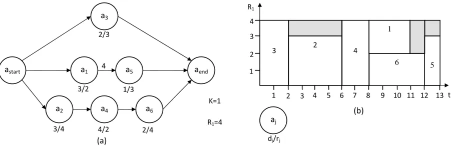
Fig. 1. An example for resource constrained project scheduling problem. The project comprising 6

activities that needs to be scheduled subject to K =1 renewable resource type with a capacity of 4

units. (a) presents the precedence graph of the activities, and (b) presents the corresponding optimal schedule of the activities

We have a set of resource types R=

{

R1,R2,....,RK

}

where each resource type k has a limited capacity

of R_k at any point of the time. During running of the project, each activity a_j requires r_j_,_k units of

resource type k during every time instant of its non-preemptable duration d_j. For the ‘project start’

and ‘project end’ activities we have r_j_,_k =0 ∀j∈

{

0,1,...,n+1

}

,∀k∈

{

1,2,...,K

}

. The objective of the

RCPSP is to find an ordering of the activities (see Fig. 1 (b)) that minimizes the makespan of the schedule Fn+₁ subject to the following constraints:

j j

j

h F d j n h P

F ≤ − , =1,..., +1; ∈ , (1)

( ) ≤ , ∈

{

1,2,...,

}

; ≥0

∑

∈At r Rk k K t

j jk

, (2)

where F_j is the finishing time of activity a_j, P_j is a set of preceding activities (or predecessors of activity a_j), A

( )

t = j∈V|F_j −d_j≤t<F_j and F_j ≥0, J =1,...,n+1 describe the constraints of decision

variables. The equation (1) enforces the precedence constraints between activities, and equation (2) enforces the resource limitation constraint.

4. Artificial Bee Colony and Its Application for RCPSP

This section presents the detailed description of the artificial bee colony algorithm to solve RCPSP. Fig. 2 presents the ABC algorithm in pseudocode. ABC algorithm uses the priority-based representation (Zhang et al., 2006) for its individuals. Each bee represents a position in the search

space. If the project has n activities, the bees will fly in the search space with n dimensions. A

position is a candidate for a priority list where each of its elements fixedly represents an activity and

astart aend

a2

a4 a6

a1

a3

a5

2/4 4

4/2 3/4

2/3

3/2 1/3

R1

4 2

6

3

5

1

1 2 3 4 5 6 7 8 9 10 11 12 13 1

2 3 4

t K=1

R1=4

dj/rj (a)

(b) aj

(5)

its corresponding value shows the priority of that activity. Hence, the position vector xr_i of each bee i

is used to represent the priority values of a schedule i with n activities. Each element d of the position vector xr_i is located between 0 and 1 (i.e. 0≤xid ≤1). Hence, each element with a value larger than 1

or smaller than 0 is set to 1 or 0, respectively.

Algorithm ABC (Population size, Scouts, Max_Trial, Prj)

_______________________________________________________________________________

Initialization

DefineFoodNumber = Population size/2 Fori = 1 toFoodNumber

Initialize food source i randomly Triali = 0

End For Repeat

For i = 1 toFoodNumber

Evaluate food source i using serial-SGS End For

(Send Employed Bees) For i = 1 toFoodNumber

Select a parameter d randomly

Select Neighbor k randomly

Calculate vid=xid+ω1rid(xid−xkd)

Evaluate new food source using serial-SGS

If the new food source presents a schedule with smaller makespan

Update the position

If the food source has not been improved

Increment its Trialby 1 End For

(Send Onlooker Bees)

Calculate probabilities for each food source using equation (5) For i = 1 toFoodNumber

Select a parameter d randomly

Select Neighbor k from food sources based on equation (5)

Calculate vid=xid+ω2rid(xid−xkd)

Evaluate new food source using serial-SGS

If the new food source presents a schedule with smaller makespan

Update the position

If the food source has not been improved

Increment its Trialby 1 End For

(Send Scout Bees)

Definei as the food source with the maximum Trial Initialize food source i randomly

Triali= 0

Until termination condition is met

Returnbest schedule

_________________________________________________________________________________

(6)

The ABC employs a population of different types of bees to find the schedule with minimum makespan. The type of a bee is defined based on the behavior she uses to find the food sources. A bee waiting on the dance area for making decision to choose a food source is called onlooker bee; the bee which goes to the food source already visited by herself just before is named as employed bee, and the bee which flies spontaneously in the search space is called scout bee. The ABC uses the following steps to find a schedule with minimum makespan:

Step 1 (Initialization): ABC receives a set of parameters as inputs: population size (Population size), number of scouts (Scouts), Max_Trial, and project (Prj). Max_Trial is the parameter used to identify the food sources that should be abandoned. At initialization step, the number of food sources (FoodNumber) will be set to half of Population size, and the population is equally subdivided as

employed bees and onlookers. Next food sources will be initialized randomly. Trial is the parameter

used to be incremented when a food source is not optimized in twoconsecutive cycles, and Prj is the

project to be scheduled.

Step 2 (Bee evaluation): At the start of each cycle, all the food sources need to be evaluated. To evaluate the fitness of a food source, we need to generate the schedule from the priority list. Hence, we need to use a schedule generation scheme (SGS). We use serial-SGS that constructs active schedules (Kolisch & Hartmann, 1999). The serial-SGS is an activity oriented scheme that generates a schedule in n stages from the priority list. Serial SGS uses two disjoint activity sets at each stage s∈

{

1,2,...,n

}

: the set of scheduled activities and the set Es of eligible activities (i.e. all activities for which all

predecessors are scheduled). In each stage, serial-SGS select one eligible activity j∈Es and schedules

it at the earliest precedence and resources feasible time. Next, the set of eligible activities and the resource profiles of partial schedule are updated.

Step 3 (Position updating): After all the bees are evaluated, each employed bee i selects another employed bee as its own neighbor. After that, a parameter d∈

{

1,2,...,n

}

will be selected randomly. Each food source will be optimized through following equation,

(

id kd

)

id id

id x r x x

v = +ω1 − , (3)

where i represents the food sources which is going to be optimized,k∈

{

1,2,...,FoodNumber

}

and

{

n

}

d∈1,2,..., is a randomly chosen index. Although k is determined randomly, it has to be different from i. The random number r_id is selected in range of [-1, 1]. Parameter ω₁ controls the production of

neighbor food sources around xid and represents the comparison of two food positions visually by a

bee. As can be seen from equation (3), as the difference between the parameters of the xid and xkd

decreases, the perturbation on the position xid is decreased, too. Thus, as the search process approaches

the optimum solution in the search space, the step length is adaptively reduced. If a parameter value produced by this operation exceeds its predetermined limit, the parameter can be set to an acceptable value. After the employed bees explore the new areas of the food sources, they come into the hive and share the nectar information of the sources with the onlooker bees waiting on the dance area. Sharing the information in the hive, an onlooker bee only needed to employ a decision making process to select one of the food sources advertised by the employed bees. For this purpose, the probability for each

food source k advertised by the corresponding employed bee will be calculated as follows,

( )

,

1

∑

=

FoodNumber

m m

k k

x

fit

x

fit

p

_r

r

(4)

where fit

( )

xr_m is the probability of the food source proposed by the employed bee k which is

proportional to the quality of the food source. The quality depends on the makespan of the schedule

(7)

( )

1 ,

m m

makespan x

fit r = (5)

where makespanm is the value of the makespan proposed by the food source m. After calculating the

probabilities, each onlooker bee employs the roulette wheel to choose a food source advertised by the

employed bee k based on its probability. By selecting a food source, the onlooker bee updates its

position using the following equation if the newly discovered food source proposes a schedule with smaller makespan than the old one,

(

id kd

)

id id

id x r x x

v = +ω2 − , (6)

where parameter ω₂ controls the importance of the social knowledge provided by the employed bees.

Under this probabilistic approach, the food sources with better schedules attract more onlooker bees. At each cycle of the algorithm, the positions are evaluated and if a food source cannot be improved

after a predetermined number of iterations (called Max_Trial), then the corresponding food source is

abandoned. The Max_Trial parameter is determined manually. In this work, the value of Max_Trial is

set to 5. The abandoned food source is replaced with the new one founded by the scouts. A scout produces a new position randomly and replaces the abandoned food source if the new food source has better nectar. Assume that the abandoned source is xi and j∈

{

1,2,...,n

}

, then the scout discovers a new

food source to be replaced with xi. This operation can be defined as follows,

id id r

v = , (7)

where rid is selected in the range of [0,1] randomly. After each candidate source position vij is

produced and evaluated by the artificial bee, its performance is compared with that of its old one. If the new food source proposes a schedule with smaller makespan than the old one, it is replaced with the new one in the memory. Otherwise, the old one is retained in the memory.

Step 4 (Termination): By termination of the ABC algorithm, the schedule with minimum makespan obtained by the population is returned as the output.

5. Computational Experiments

This section presents the experiments conducted to investigate the performance of ABC and the other algorithms on RCPSP datasets in PSPLIB. We have used several problem instances which are successfully solved by an algorithm as a measure for performance comparison. This measure differs

from the other measure so-called average deviation from the optimal solution used in literature for

performance comparison. Hence, we need to implement the investigated meta-heuristic approaches.

To investigate the performance of our ABC-based algorithm1, we implement some of the most

representative meta-heuristics for solving RCPSP problems in java: ant colony optimization (ACO) (Chen et al., (2006)), genetic algorithm (GA) (Hartmann, 1998), standard particle swarm optimization (PSO) (Zhang et al., 2005), PSO+ (Chen et al., 2010), OOP-GA (Montoya-Torres et al., 2010), GAPS (Mendes et al., 2009), ANGEL (Tseng & Chen, 2006), and ACOSS (Chen et al., 2010), Neurogenetic

(Agrawal et al., 2010). The experiments were executed on a Core 2 Duo 1.66 GH Pentium.We have

used well-known scheduling case studies from PSPLIB to evaluate performance of the algorithms. PSPLIB involves three case studies j30, j60, and j90 that consist of 480 problem instances with four resource types and 30, 60, and 90 activities, respectively. Also PSPLIB involve j120 case study that

1

(8)

consists of 600 problem instances with four resource types and 120 activities. We have tested ten approaches under the following configurations.

5.1. Experimental Settings

In our experiments, each algorithm is configured under parameters values which result the best performance. In this section we specify these suitable parameter values. For the proposed ABC-based

algorithm, parameters such as coefficients ω1 and ω2, population size, number of iterations, and

Max_Trial influence the performance of this algorithm. To determine the suitable parameter values, we conduct two experiments to study the effects of the ABC parameters while solving problem

instances of the j30, j60, j90, and j120 case studies. Our empirical studies have shown that Max_Trial

has not significant effect on the performance of our algorithm. Hence, we exclude it from our analysis. In the first experiment, the performance of the proposed algorithm is studied under different values of the coefficients ω1 and ω2. These parameters vary from 0.6 to 1.4 with the step size of 0.2. The population size and the iteration number are set to 100 and 50, respectively. Fig. 3 shows the

effect of coefficients ω1 and ω2 on the performance of our algorithm. The vertical axis shows the

number of problem instances which are successfully solved by our algorithm, and the horizontal axis

shows the coefficient ω2. The results show that these two parameters have the positive effect on the

performance of the algorithm. The best results are obtained for ω₁=0.8 and ω₂=1.2. Our empirical study have shown that the quality of the algorithm decreases when both the parameters are set to values larger than 1.4. Also, the quality of the algorithm decreases when ω₁ has a small value and ω₂ has a large vale. Hence, we recommend using the proposed algorithm under following configuration:

9 . 0 7

.

0 ≤ω₁≤ and 1.1≤ω2≤1.3.

(a) j30 case study (b) j60 case study

(c) j90 case study (d) j120 case study

Fig. 3. The effect of coefficients ω₁ and ω₂ on the performance of the ABC algorithm

375 380 385 390 395 400

0.6 0.8 1 1.2 1.4

w2

qual

it

y

w1=0.6 w1=0.8 w1=1.0 w1=1.2 w1=1.4

310 312 314 316 318 320 322 324 326 328 330

0.6 0.8 1 1.2 1.4

w2

qual

it

y

w1=0.6 w1=0.8 w1=1.0 w1=1.2 w1=1.4

310 311 312 313 314 315 316 317 318 319 320

0.6 0.8 1 1.2 1.4

w2

qu

al

it

y

w1=0.6 w1=0.8 w1=1.0 w1=1.2 w1=1.4

100 102 104 106 108 110 112 114

0.6 0.8 1 1.2 1.4

w2

qual

it

y

(9)

We have conducted the second experiment to observe if the performance of our algorithm under fixed number of schedules is affected by the number of iterations or population size. Here, both the values of the population size and the number of iterations are varied from 10 to 250 subject to the following constraint: the number of produced schedules is fixed at 2500. The population size varies in steps of

10, and for each of them the corresponding number of iterations computed as _⎢⎢⎡2500_pop_{_}_size_⎥⎥⎤. The

first experiment shows that the best results are obtained for ω₁=0.8 and ω₂ =1.2, hence we use these values. Table 1 shows the effect of population size and the number of iterations on the performance of our algorithm. The results show that the quality of our algorithm is relatively affected by these two parameters. The percentage of problem instances successfully solved by our algorithm varies in range of [78.13%, 78.75%], [66.20%, 67.29%], [64.80%, 65.42%], and [17.67%, 18.50%] for j30, j60, j90, and j120 case studies, respectively. The success rate implies that although one can obtain better result by fine tuning the number of iteration and size of the population, the rate of improvement is not significant under fixed number of schedules. Hence we can say that the proposed algorithm provides stability in solving RCPSP under fixed number of schedules. As a result, the parameters of the ABC algorithm are set as follows:

For the ABC algorithm, the population is equally subdivided into the employed and onlooker bees and one individual is selected as scout bee. The parameter ω₁ and ω₂ are respectively set to 0.8 and

1.2. The value of Max_Trial is set to 5 manually. The population size is set at 100, and each case

study was tested 15 trials. Other algorithms' parameters are set as follows:

The parameters of ACO algorithm are set as: τ0 =0.5, q0 =0.9, q1=0.9, α =1, β =1, c=10, δ =0.1, and ρ =0.1 . For genetic algorithm, the mutation probability is set to 0.4, and two-point crossover is used.

For particle swarm optimization, the maximum and minimum values of inertia weight (i.e. w_max and

min

w ) are set to 0.9 and 0.4, respectively. The linear inertia weight is used here where the inertia

weight linearly decreases from wmax to wmin throughout iterations. The particles are positioned

randomly in range of [0,1] at initial time, and the initial velocity of each particle is set to 0. The acceleration coefficients c1 and c2 are set to 0.85.

Table 1

The effect of population size and number of iterations on the performance of the proposed ABC algorithm

Population size 10 20 30 40 50 60 70 80 90 100

#iterations 250 125 83 63 50 42 36 31 28 25

Success rate

j30 78.54% 78.54% 78.33% 78.75% 78.75% 78.54% 78.54% 78.55% 78.13% 78.13%

j60 67.29% 67.09% 66.45% 66.25% 66.62% 66.25% 66.62% 66.58% 66.45% 66.25%

j90 65.42% 65.63% 65.42% 65.63% 65.21% 65.00% 65.21% 64.80% 65.21% 64.80%

j120 18.50% 17.67% 18.50% 18.33% 18.00% 17.83% 17.83% 18.17% 18.33% 17.67%

The PSO+ is tested under the following configuration: the inertia weight w and the learning factors

1

c and c2 are set to 0.7, and the parameters

q

0 and

q

'

are set to 0.05 and 0.95, respectively.

(10)

next generation, and the bottom 20% of the population chromosomes are replaced with randomly generated chromosomes. The ACOSS method is tested based on the following control parameters: decay factor ρ is set to 0.02, the control parameters α , β are set to 1 and 2.5, respectively, and the pheromone trail limits are selected as the way reported by Chen et al. (2010). For the Neurogenetic method, the learning rate is set to 0.05, the weights are initialized at 1, two-point crossover is used for its GA part and mutation probability is set to 0.5. The number of interleaving is set to 5, the proportion of GA is taken as 90%, and the number of GA solutions to feed NN is used as four.For the ANGEL method, the parameters Loop_limit and Generation_limit are set to 3 and 5, respectively. Other parameters are set as: α =0.9, ρ=0.1, Δini =0.00001, Pcro=0.75, and Pmutl =0.05. We have

used two stopping criteria in our experiments. An algorithm stops if the founded solution is equal to the lower bound which the critical path calculated without resource constraints or if a predetermined number of maximum of iterations are reached. In our experiments, the results are obtained for 10, 50, and 500 iterations.

5.2. Comparative Study

The following experiments were conducted to see how many cases of PSPLIB library can be solved by the proposed algorithm. We say that a case study is solved if the algorithm finds optimal solution or lower bound solution for that case study. Tables 2-5 present the experimental results for the j30, j60, j90, and j120 case studies. Each cell of a table indicates the percentage of the problem instances which are successfully solved by an algorithm.

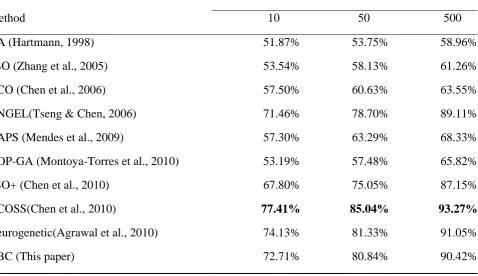
Table 2

The results of using GA, PSO, ACO, ANGEL, GAPS, OOP-GA, PSO+, ACOSS, Neurogenetic and ABC for j30 cases study

Number of iterations

Method 10 50 500

GA (Hartmann, 1998) 51.87% 53.75% 58.96%

PSO (Zhang et al., 2005) 53.54% 58.13% 61.26%

ACO (Chen et al., 2006) 57.50% 60.63% 63.55%

ANGEL(Tseng & Chen, 2006) 71.46% 78.70% 89.11%

GAPS (Mendes et al., 2009) 57.30% 63.29% 68.33%

OOP-GA (Montoya-Torres et al., 2010) 53.19% 57.48% 65.82%

PSO+ (Chen et al., 2010) 67.80% 75.05% 87.15%

ACOSS(Chen et al., 2010) 77.41% 85.04% 93.27%

Neurogenetic(Agrawal et al., 2010) 74.13% 81.33% 91.05%

ABC (This paper) 72.71% 80.84% 90.42%

(11)

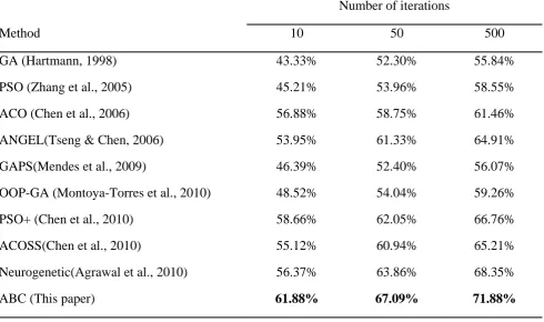
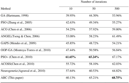
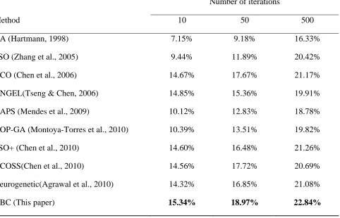
results to ACOSS approach. The ABC approach obtains the third rank on j30 case study after 10, 50, and 500 iterations. Table 3 summarizes the results of our approach and the other meta-heuristics approaches for j60 cases study after predetermined number of iterations. The best results for the problem instances of this case study are found by ABC algorithm. From the results we can see that the performance of the algorithms decreases as the number of activities increases. Table 4 demonstrates the experimental results of all 480 instances for j90 cases study with 90 activities after 10, 50, and 500 iterations. The PSO+ approach surpass other algorithms for 10 and 50 iterations. The second rank was obtained by ABC approach for 10 and 50 iterations. However, similar to j60 case study, ABC approach outperforms other algorithms after 500 iterations. The last case study with 120 activities is the most difficult case study to solve. Table 5 summarizes the results of our approach and the other meta-heuristics approaches for this case study after predetermined number of iterations. The results show that the approaches have the least performance on this case study compared to other

ones.The ABC approach provides schedules with better qualities for j120 case study.

Table 3

The results of using GA, PSO, ACO, ANGEL, GAPS, OOP-GA, PSO+, ACOSS, Neurogenetic, and ABC for j60 cases study

Method 10 50 500

GA (Hartmann, 1998) 43.33% 52.30% 55.84%

PSO (Zhang et al., 2005) 45.21% 53.96% 58.55%

ACO (Chen et al., 2006) 56.88% 58.75% 61.46%

ANGEL(Tseng & Chen, 2006) 53.95% 61.33% 64.91%

GAPS(Mendes et al., 2009) 46.39% 52.40% 56.07%

PSO+ (Chen et al., 2010) 58.66% 62.05% 66.76%

ACOSS(Chen et al., 2010) 55.12% 60.94% 65.21%

ABC (This paper) 61.88% 67.09% 71.88%

In our experiments, we used 2040 problem instances from four categories of case studies.To view the

overall performance of the proposed algorithm, its ability in solving all the problem instances is considered. Fig. 4 presents the average percentage of the problem instances which are successfully solved by the algorithms after 10, 50, and 500 iterations. From the results, it can be seen that the proposed algorithm surpasses the PSO+, ANGEL, ACOSS, and Neurogenetic algorithms and successfully outperforms the other ones.

(12)

that ABC outperforms other meta-heuristics investigated in this paper. This happens due to the ability of ABC algorithm in providing better diversity throughout the execution of the algorithm. Providing appropriate level of diversity helps the algorithm to alleviate the deficiencies of meta-heuristic algorithm such as stagnation and premature convergence and consequently provide the ability to explore further regions of the search space to find better solutions.

Table 4

Method 10 50 500

GA (Hartmann, 1998) 39.95% 44.30% 53.96%

PSO (Zhang et al., 2005) 42.63% 49.34% 55.27%

ACO (Chen et al., 2006) 54.25% 57.92% 59.80%

ANGEL(Tseng & Chen, 2006) 53.08% 58.23% 61.49%

GAPS (Mendes et al., 2009) 45.85% 48.72% 54.21%

PSO+ (Chen et al., 2010) 61.65% 65.24% 67.17%

ACOSS(Chen et al., 2010) 55.72% 58.10% 62.03%

ABC (This paper) 60.13% 65.21% 68.75%

#iterations = 10 #iterations = 50 #iterations = 500

Fig. 4. Overall performance of the ABC and the other algorithms investigated in this paper

0 0.1 0.2 0.3 0.4 0.5 0.6

GA PSO AC

O

AN

G

E

L

G

APS OOP

-G

A

AC

O

S

N

eur

o

genet

ic

PSO

+

ABC 0

0.1 0.2 0.3 0.4 0.5 0.6

GA PSO AC

O

AN

G

E

L

G

APS OOP

-G

A

AC

O

S

N

e

u

rog

en

et

ic

PSO

+

ABC 0

0.1 0.2 0.3 0.4 0.5 0.6 0.7

GA PS

O

AC

O

AN

G

E

L

GA

P

S

OO

P

-G

A

AC

O

S

N

eur

ogeneti

c

PS

O

+

AB

(13)

Table 5

Method 10 50 500

GA (Hartmann, 1998) 7.15% 9.18% 16.33%

PSO (Zhang et al., 2005) 9.44% 11.89% 20.42%

ACO (Chen et al., 2006) 14.67% 17.67% 21.17%

ANGEL(Tseng & Chen, 2006) 14.85% 15.36% 19.91%

GAPS (Mendes et al., 2009) 10.12% 12.83% 18.78%

PSO+ (Chen et al., 2010) 14.60% 16.48% 21.26%

ACOSS(Chen et al., 2010) 14.56% 17.72% 20.69%

ABC (This paper) 15.34% 18.97% 22.84%

6. Conclusions

In this paper we have considered the performance of the artificial bee colony meta-heuristic on resolving the single-mode resource constrained project scheduling problem. The ABC-based meta-heuristic starts with a set of initial schedules and tries to improve them cycle by cycle by applying four-step strategy as described in the paper. We have evaluated the performance of ABC strategy on PSPLIB case studies against other meta-heuristics. Our experimental results prove that ABC provides an efficient way for solving RCPSP. Moreover, the better performance can be obtained using ABC strategy for large-sized case studies. The competitive results obtained by the ABC-based meta-heuristic on solving RCPSP may encourage one to study alternatives for improving the performance of ABC-based approach as a newly emerged meta-heuristics.

Acknowledgment

(14)

R A A A A A B B B B C C C C D D D F K References Abbasi, B., with ro 146–1 Agarwal, A projec Akbari, R., numer Numer

Ashtiani, B resour Journa Alatas B.(2 with A Blazewicz constr Boctor, F. schedu Boctor, F. constr 2335– Bouleimen, constr Opera

Chen, R. M schem

Applic

Chen, R. M preced 297. Chen, R. M

schem

Applic

Chen, W., S resour Damak, N., resour – 2659 Debels, D., Constr Debels, D. /Electr Resear

Fekete, S. P

Notes

Karaboga, D optimi 471.

Shadrokh, obustness a

52.

A., Colak, S. ct scheduling

Mohamma rical functi

rical Simula

B., Leus, R rce-constrain

al of Schedu

010). Chao

Applications

J., Lenstra raints: classi

F.(1990). uling. Europ

F.(1996). A rained proje –2351.

K., & Leco rained proje

ational Rese

M., Wu, C. L me to solve

cations, 37, M., Lo, S. T

dence and re

M., Wu, C. L me to solve

cations, 37, Shi, Y. J., T rce-constrain Jarboui, B. rce-constrain

9.

, & Vanho rained Proje ., De Rey romagnetism

rch, 169, 63 P., & Schep

in Compute

D., & Bast ization: arti

S., & Ark and makesp

., & Erengu g problem. adi, M., & on optimiz

ation, 15, 3 ., & Aryan ned project

uling, doi: 1

otic bee col

s, 37, 5682-J. K., & ification and Some effi pean Journa An adaptat ect scheduli ocq, H.(199 ect scheduli

earch, 149, 2 L., Wang, C

resource-c 1899–1910 T., Wang, C

esources co

L., Wang, C resource-c 1899–1910 Teng, H. F.

ned project ., Siarry, P. ned project

oucke, M.(2 ect Schedul yck, B., L

m meta–he 38-653. pers, J.(1998

er Science, turk, B.(20 ificial bee c

kat, J.(2006 an criteria.

uc, S.(2010)

Computers

Ziarati, K.( zation. Jour

142-3155. nezhad, M. t schedulin 10.1007/s10 ony algorith 5687.

Rinnooy K d complexit cient multi

al of Opera

tion of the ing problem

93). A new e ing problem

268–281. C. M., & Lo constrained 0.

C. J., & Wu nstraints by

C. M., & Lo constrained 0.

, Lan, X. P scheduling , & Loukil, scheduling

2004). An ing Problem Leus, R.,

uristic for

8). New cla 1412, 257–2 007). A pow

colony (ABC

6). Bi-objec

Journal of

). A Neurog

& Operatio

(2010). A n

rnal of Co

B.(2009). ng problem

0951-009-01

hms for glo

Kan A. H. ty. Discrete

i-heuristic

ational Rese

simulated ms. Interna

efficient sim m and its m

o, S. T.(201 scheduling

u, C. L.(20 y ant colony

o, S. T.(201 scheduling

P., & Hu, L g. Informatio

T.(2009). D g problems.

Electromag m. Lecture N

& Vanhou project sch

asses of low 270. werful and C) algorithm ctive resour Applied Ma genetic appr ons Researc

novel bee s

ommunicati New comp m: exploring 143-7. obal numer G.(1983).

e Applied M

procedures

earch, 49, 3– annealing

ational Jour

mulated ann multiple mo

10). Using n g problem i

006). Multip y system. Pr

10). Using n g problem i

. C.(2010).

on Sciences

Differential

Computers

gnetism M

Notes on Co

ucke M.(2

heduling. E

wer bounds f

d efficient a m. Journal

ce-constrain

athematics a

roach for th

ch, doi:10.1

swarm optim

ions on No

petitive res g the benef

rical optimi Scheduling Mathematics, for resou –13. algorithm

rnal of Pro

nealing algo ode version novel partic in PSPLIB processor sy roceeding of novel partic in PSPLIB An efficien

s, 180, 1031 l evolution f

& Operatio

eta-Heuristi

omputer Sci

006). A h

European Jo

for bin-pack

algorithm f

of Global O

ned project and Compu he resource-016/j.cor.2 mization al onlinear Sc

sults for the fits of

pre-zation. Exp

g projects , 5, 11–24. urceconstrain

for solvin

oduction Re

orithm for th . European

cle swarm o . Expert Sy

ystem sche

of ICS Confe

cle swarm o . Expert Sy

nt hybrid al –1039. for solving

ons Researc

ic For The

ience, 3871, hybrid sca

Journal of O

king proble

for numeric

Optimizatio

t scheduling

utation, 180

-constrained 010.01.007 lgorithm for ciences and e stochastic -processing pert Systems to resource ned projec ng resource

esearch, 34

he resource

n Journal of

optimization

ystems with

eduling with

erence, 292

optimization

ystems with

lgorithm for

multi-mode

ch, 36, 2653

e Resource , 259-270. atter search

Operationa

ms. Lecture

cal function

(15)

K K K K H H M M M M M M N P P R R Karaboga, D Mathe Kolisch, R., schedu Schedu 147–1 Kolisch, R. Journa Krüger, D., projec Opera Hartmann, S projec Hartmann, Naval Mahdi Mob an enh Soft C Mendes, J. the res 92–10 Mendes, J. the res 92–10 Mingozzi, A

schedu Manag Mobini, M. schedu doi:10 Montoya-To with li 28, 61 Neumann, scheduli 2, 325-3 Pan, Q. K., algorit

doi:10

Pham, D. T manip 493–4 Rabbani, M constr

Journa

Ranjbar, M. approa

D., & Akay

ematics and

, & Hartma uling probl

uling: Rece

78.

(1996). Eff

al of Opera

& Scholl, ct schedulin

ational Rese

S., & Brisko ct scheduling S.(1998). A

Research L

bini, M. D., hanced scat

Computing, 1 J., Gonalve source cons 09. J., Gonalve source cons 09. A., Maniezz uling with gement Scie

., Mobini Z uling pro

0.1016/j.aso

orres, J. R., imited resou

9–628. K., Schwin ing with no 343.

M. Tasgeti thm for th

0.1016/j.ins.

T., Castellan pulator using 498.

M., Fatemi G rained proje

al of Opera

.(2008). Sol ach. Journa

y, B.(2009). d Computati nn, S.(1999 lem: classi ent Models, ficient prior tions Mana

A.(2009). A ng problem

earch, 197, 4 orn, D.(201 g problem. A competiti

Logistics, 45 Rabbani, M tter search 13, 597–610 es, J. F., & R

strained pro

es, J. F., Re strained pro

zo, V., Ric resource co

ence, 44, 71 Z., & Rabb oblem un

c.2010.06.0

, Gutierrez-urces using

ndt, C., & nregular ob

iren F., Sug he lot-strea

.2009.12.02

ni, M., & F g the bees a

Ghomi, S.M ect scheduli

tional Rese

lving the re

al of Applied

. A compar

on, 214, 10 9). Heuristic

fication an

algorithms

rity rules fo

agement, 14 A heuristic m with sequ

492–508. 0). A surve

European J

ive genetic 5, 733– 750 M., Amalnik algorithm 0.

Resende M oject schedu

esende, M. G oject schedu

cciardelli, S onstraints b

4–729. bani M.(20 nder resou

013.

-Franco, E., a genetic a

Zimmerma bjective func ganthan, P. aming flow 25. Fahmy, A. algorithm. I

M.T., Jolai, ing in stoch

arch, 176, 7 esource-con d Mathemat ative study 8-132. c algorithm nd computa and Applic

or the resou , 179–192.

solution fr uence-depen

ey of varian

Journal of O

algorithm 0.

k, M. S., Raz for a resou

M.G.C.(2009 uling probl

G. C.(2009) uling probl

S., & Bianc based on a

010). An A urce con

, & Pirachi algorithm. In

ann, J.(200 ctions. Euro

N., & Chua w shop sch

A.(2008).

IEEE intern

F., & Lahij hastic netw 794–808. nstrained pro

tics and Com

of Artificia

s for solvin ational ana

cations, Klu

urce-constra

amework fo ndent trans

nts and exten

Operational

for resour

zmi, J., & R urce-constra

9). A random em. Compu

). A random em. Compu

co, L.(1998) new math Artificial Im nstraints. ca N-Mayo nternationa 03). Order-b opean Journ

a, T. J.(201 heduling p

Learning th

national con

ji, N.S.(200 works using

oject schedu

mputation, 2

al Bee Colo

ng the resou lysis. J. W

uwer Acade

ained projec

or the resou sfer times.

nsions of th

l Research, ceconstrain

Rahimi-Vah ained projec

m key based

uters & Op

m key based

uters & Op

). An exact hematical fo

mmune Algo

Applied

orga, C.(201

al Journal of

based neig

nal of Oper

0) A discre

problem, In

he inverse

nference on

07). A new critical cha uling proble 201, 313–3 ony algorith urce-constra Weglarz (Ed mic Publish ct schedulin urce constra European he resource-207, 1-14. ned project

hed, A. R.(2 ct schedulin

d genetic al

erations Re

d genetic al

erations Re t algorithm ormulation. orithm for Soft Com 10). Project

of Project M

ghborhoods rational Res ete artificial nformation kinematics industrial

heuristic fo ain concept

em using fi 18.

hm. Applied

ained projec d.), Projec hers, Berlin

ng problem

ained multi

Journal of

-constrained

scheduling

2009). Using ng problem

lgorithm for

esearch, 36

lgorithm for

esearch, 36

m for projec

Journal of

the projec

mputing,

t scheduling

Management

for projec

search, 149

l bee colony

Sciences.

of a Robo

informatics

or resource t. European

(16)

Sprecher, A.(2000). Scheduling resource-constrained projects competitively at modest memory

requirements. Management Science, 46, 710–723.

Stork, F., & Uetz, M.(2005). On the generation of circuits and minimal forbidden sets. Mathematical

Programming, 102, 185–203.

Teodorovic, D., & Dell Orco, M.(2007). Bee colony optimization–a cooperative learning approach to

complex transportation problems. Advanced OR and AI Methods in Transportation, 51–60.

Teodorovic, D., Panta, L., Goran M., & Dell, O. M.(2006). Bee colony optimization: principles and applications. Proceeding of eighth seminar on neural network applications in electrical engineering, Neurel, 151–156.

Thomas, P., R., & Salhi S.(1998). A tabu search approach for the resource constrained project

scheduling problem. Journal of Heuristics, 4, 123–139.

Tormos, P., & Lova, A.(2001). A competitive heuristic solution technique for resource-constrained

project scheduling. Annals of Operations Research, 102, 65–81.

Tseng, L.Y., & Chen, S. C.(2006). A hybrid metaheuristic for the resource-constrained project

scheduling problem, European Journal of Operational Research, 175, 707–721.

Valls V., Ballestın F., & Quintanilla, S.(2008). A hybrid genetic algorithm for the

resource-constrained project scheduling problem. European Journal of Operational Research, 185, 495–

508.

Zhang, H., Li, X., Li, H., & Huang, F.(2005). Particle swarm optimization-based schemes for

resource-constrained project scheduling. Journal of Automation in Construction, 14, 393– 404.

Zhang, H., Li, H., & Tam, C. M.(2006). Particle swarm optimization for resource-constrained project