Learning Accurate and Interpretable Classifiers Using Optimal Multi-Criteria Rules

(1)

Learning Accurate and Interpretable Classifiers

Using Optimal Multi-Criteria Rules

Itamar Hata, Adriano Veloso, Nivio Ziviani

Computer Science Department, Universidade Federal de Minas Gerais, Brazil {itamar, adrianov, nivio}@dcc.ufmg.br

Abstract. The Occam’s Razor principle has become the basis for many Machine Learning algorithms, under the interpretation that the classifier should not be more complex than necessary. Recently, this principle has shown to be well suited to associative classifiers, where the number of rules composing the classifier can be substantially reduced by using condensed representations such as maximal or closed rules. While it is shown that such a decrease in the complexity of the classifier (usually) does not compromise its accuracy, the number of remaining rules is still larger than necessary and making it hard for experts to interpret the corresponding classifier. In this paper we propose a much more aggressive filtering strategy, which decreases the number of rules within the classifier dramatically without hurting its accuracy. Our strategy consists in evaluating each rule under different statistical criteria, and filtering only those rules that show a positive balance between all the criteria considered. Specifically, each candidate rule is associated with a point in ann-dimensional scattergram, where each coordinate corresponds to a statistical criterion. Points that are not dominated by any other point in the scattergram compose thePareto frontier, and correspond to rules that are optimal in the sense that there is no rule that is better off when all the criteria are taken into account. Finally, rules lying in the Pareto frontier are filtered and compose the classifier. Our Pareto-Optimal filtering strategy may receive as input either the entire set of rules or even a condensed representation (i.e., closed rules). A systematic set of experiments involving benchmark data as well as recent data from actual application scenarios, followed by an extensive set of significance tests, reveal that the proposed strategy decreases the number of rules by up to two orders of magnitude and produces classifiers that are extremely readable (i.e., allow interpretability of the classification results) without hurting accuracy.

Categories and Subject Descriptors: I.2.6 [Artificial Intelligence]: Learning; H.28 [Database Applications]: Data mining; I.7 [Document and Text Processing]: General

Keywords: association rules, classification, Pareto frontier

1. INTRODUCTION

The classification task builds an abstract model from labeled data (i.e., the training-set), and then apply such abstract model (aka., classifier) for predicting unknown (discrete) variables in the data (i.e., the test-set). Historically, the typical goal of classification algorithms is to maximize accuracy as much as possible, often by building classifiers that are not readable, such as KNNs [Cover and Hart 1967], SVMs [Cortes and Vapnik 1995; Joachims 2006], and Naive Bayes [Domingos and Pazzani 1997; Lowd and Domingos 2005]. In several application scenarios, however, the ability to interpret the classification result is increasingly becoming as important as the ability to classify correctly. For instance, in diagnosis of lung cancer the doctor must know features that were decisive in the prediction [Mramor et al. 2007]. Other applications in which the readability of the classifier is of paramount importance include fraud detection, credit analysis and impact analysis of marketing campaigns.

Interpretable classifiers are mainly represented by decision trees [Breiman et al. 1984; Gehrke et al. 1999] and by associative classifiers [Liu et al. 1998]. However, modeling large and complex datasets

(2)

using tree-like structures and rule-sets usually results in large and possibly hard-to-read models. Learning associative classifiers on a demand-driven basis [Menezes et al. 2010; Veloso and Meira Jr. 2011] comes as an alternative to this problem: instead of building a single and unnecessarily complex rule-set that explains the entire training-set, several simpler rule-sets are built, where each rule-set explains a subset of the training-set which is relevant to a specific test instance, resulting in one classifier (i.e., model) for each test instance. It can be shown that the number of rules that compose each classifier increases polynomially with the number of distinct features in the training-set [Veloso et al. 2006], but this still corresponds to an exponential growth with the number of features within the test instance. This exponential dependence may challenge the readability of the classifiers, and thus the problem we address in this paper is how to ensure readability of associative classifiers without compromising their accuracy.

Our proposed strategy lies on assessing the utility (or efficiency) of each rule in the original rule-set by evaluating it under different statistical criteria. Such criteria include important rule statistics [Tan et al. 2002], namely: support, confidence, added-value, and Yule’s Q. Intuitively, we want to select those rules that provide the best trade-off or balance amongst these four criteria. The proposed strategy for filtering efficient rules is based on the concept of Pareto Efficiency [Palda 2011]. This is a central concept in Economics, which informally states that “when some action could be done to make at least one person better off without hurting anyone else, then it should be done.” This action is called Pareto improvement, and a system is said to be Pareto-Efficient (or Pareto-Optimal) if no such improvement is possible. The same concept may be exploited for the sake of selecting efficient rules. In this case, each candidate rule is associated with a point in an-dimensional space (or scattergram), which we callrule-utility space. Each dimension in this space corresponds to one of the four statistical criteria used. Points that are not dominated by any other point in this space compose the Pareto Frontier [Corne et al. 2000]. Points lying in the frontier correspond to rules for which no Pareto improvement is possible, being therefore optimal rules in the sense there is no rule that is better off when all the criteria are taken into account. Optimal rules are selected and compose the final classifier.

We conducted a systematic evaluation involving benchmark data from the UCI repository [Bache and Lichman 2013], as well as real data obtained from more challenging application scenarios, such as sentiment stream analysis [Pak and Paroubek 2010; Santana et al. 2011]. Our experiments revealed that the proposed filtering strategy based on optimal multi-criteria rules is extremely effective, drasti-cally decreasing the complexity of the classifiers by reducing the number of rules by up to two orders of magnitude. Also, our filtering strategy may be coupled with condensed representations, such as closed rules. Further, an extensive set of significance tests indicates that the accuracy achieved by these simpler classifiers is statistically equivalent to the accuracy obtained by typically more complex classifiers. As a result, classification is still effective but the underlying model is extremely readable.

The specific contributions of this paper are summarized as follows:

—Instead of using ad hoc utility measures in order to assess the importance of each rule, we propose a rule-utility space. Rules are selected from such space based on the concept of Pareto-Efficiency.

—Our rule filtering strategy is in accordance with the Occam’s Razor principle [Blumer et al. 1987; Domingos 1999; Zah´alka and Zelezn´y 2011], since it significantly decreases the complexity of the final classifier, without hurting its classification performance.

—An extensive set of experiments, in which we evaluate the accuracy and interpretability of the classifiers. Our findings are supported by a proper set of significance tests.

(3)

2. BACKGROUND AND RELATED WORK

In this section we introduce the main concepts that we used to formulate our rule filtering strategy.

2.1 The Occam’s Razor Principle and the Cost of Complexity

Informally, the Occam’s Razor principle states that “all else being equal, simpler explanations are better.” In the context of machine learning and the theory of prediction, this idea can be made precise by choosing appropriate definitions for “equal”, “simpler” and “better”. One difficulty, however, is that many different definitions are possible. Simplicity, for instance, is typically given as a function of the syntactic size of the classifier: the number of nodes in a decision tree, the number of conditions in a rule-set, or, in general, the number of parameters in the classifier [Domingos 1999]. Unfortunately, no fully satisfactory computable definition of simplicity exists, and perhaps none is possible. Thus, in this paper we will be concerned with the heuristic view of simplicity above.

Definitions for “equal” and “better” are also problematic [Lattimore and Hutter 2011]. We may consider, for instance, that a classifier is better than other if the first provides lower training-set error. This definition, however, may lead to problems such as overfitting, since the best classifier would be the one with the lowest training-set error. Thus, in this paper we will compare classifiers considering approximations of their generalization error (i.e., by means of cross-validation). Finally, we also consider that a classifier is better than other only if its generalization error is significantly smaller, and thus in this paper we will employ a proper set of significance tests in order to assure statistical difference between the classifiers.

2.2 Associative Classifiers and Demand-Driven Rule Extraction

Despite all the discussion concerning Occam’s Razor and machine learning, there is another good reason for preferring simpler models and classifiers: they are easier for people to understand, remember and use (as well as cheaper for computers to store and manipulate). Readability and comprehensibility, however, are not solely dependent on model complexity−some classifiers, although simple, are still unreadable. Classification models produced by SVM, KNN or Bayesian algorithms, are not readable, no matter how simple are the models. Although nomograms [Mozina et al. 2004; Jakulin et al. 2005] can be useful tools for enabling the visualization of these models, they are still problematic for high-dimensional problems. Decision trees, on the other hand, are a representative of classifiers that are naturally readable−each path from the root node to a leaf corresponds to a decision or a prediction. However, modeling large and complex datasets using tree-like structures results in large and possibly hard-to-read models with many possible paths.

Associative classifiers appear as an alternative to decision trees, since they are highly effective and naturally readable. The classifier (which we denote asR) is composed of rules [Agrawal et al. 1993] of the form{X −→y}, whereX is a feature-set andyis the class variable. Such rules are extracted from the training-set (which we denote asD) and then used to perform predictions, that is, rules inRare collectively used to approximate the likelihood of an arbitrary example belonging to classy. Basically,

Ris interpreted as a poll, in which each rule{X −→y} ∈ Ris a vote given byX for a specific classy. Given an examplexin the test-set, a rule{X −→y}is only considered a valid vote if it is applicable tox.

Definition 1: A rule {X −→y} ∈ R is said to be applicable to example xif X ⊆x. That is, if all features inX are present in examplex.

We denote asRxthe set of rules inRthat are applicable to examplex. Thus, only and all the rules in Rx are considered as valid votes when classifyingx. Further, we denote as Ryx the subset of Rx containing only rules predicting classy. Votes in Ry

(4)

associated with the corresponding rules. The weighted votes fory are averaged, giving the score for

ywith regard tox, as shown in:

s(x, y) =Xθ(X→− y), where θ(r) represents a statistics associated with ruler. (1)

Finally, the likelihood ofxbeing a member of classy is given by the normalized score:

ˆ

p(y|x) = s(x, y)

s(x, y) +s(x, y) (2)

Training Projection and Demand-Driven Rule Extraction. Demand-driven rule extrac-tion [Veloso et al. 2006; Veloso and Meira Jr. 2011] is a recent strategy used to avoid the huge search space for rules, by projecting the training-set D according to the example being processed. More specifically, rule extraction is delayed until an examplexis given for classification. Then, fea-tures inxare used as a filter which configures the training-set D in a way that only rules that are applicable toxcan be extracted. This filtering process produces a projected training-set, denoted as

Dx, which contains only features that are present inx. As shown by Menezes et al. [2010], the number of rules extracted using this strategy grows polynomially with the number of distinct features inD.

Extending the Classifier Dynamically. With demand-driven rule extraction, the classifier R

is extended dynamically as examples are given for classification. InitiallyRis empty; a subset Rxi is appended to R every time an example xi is processed. Thus, after processing a sequence of m examples{x1, x2, . . . , xm}, the classifierRis{Rx1∪ Rx2∪. . .∪ Rxm}.

2.3 Rule Statistics and Rule-Utility Space

According to Equation 1, a statistics is used in order to assess the utility of a rule. Intuitively, the more utility a rule{X −→y}has, the more heavily it contributes to the score associated withy. There is a number of possible rule statistics, as pointed out by Tan et al. [2002]. Next we define four statistics that are particularly important for the sake of learning associative classifiers.

Definition 2: The confidence of a rule {X −→y} measures its accuracy in the training-setD, or, in other words, the probability of classy given the features inX.

Definition 3: The support of a rule {X −→y} measures the fraction of examples in the training-set Din which{X∪y}appears.

Definition 4: The added-value of a rule {X −→y} measures the gain in accuracy obtained by using the rule instead of always predicting classy.

Definition 5: Yules’Q is a measure commonly used to evaluate games. More specifically, given two players it evaluates the association between their bets. The Yules’Q of a rule {X −→ y} takes into account players X and X, and consider possible bets as y and y. The values assumed by Yules’Q range from perfect negative correlation betweenX andy, to perfect positive correlation.

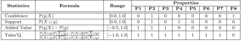
Table I shows how the four rule statistics are mathematically expressed. Researchers have exten-sively studied what are the key properties associated with an arbitrary statistics S (including the aforementioned statistics). Next, eight of these properties will be discussed. The first three were introduced by Piatetsky-Shapiro [1991].

P1. : S= 0 ifX andyare statistically independent.

(5)

Table I: Rule statistics and their properties.

Statistics Formula Range Properties

P1 P2 P3 P4 P5 P6 P7 P8

Confidence P(y|X) [0.0,1.0] 0 1 0 0 0 0 0 1

Support P(X∪y) [0.0,1.0] 0 1 0 1 0 0 0 0

Added Value P(y|X)−P(y) [−0.5,1.0] 1 1 1 0 0 0 0 0

Yules’Q P(X∪y)P(X∪y)−P(X∪y)P(X∪y)

P(X∪y)P(X∪y)+P(X∪y)P(X∪y) [−1.0,1.0] 1 1 1 1 1 1 1 0

P3. : S monotonically decreases with_P(X) or_P(y), given that_P(X, y), _P(X) or _P(y) remain the same.

The next five properties were introduced by Tan et al. [2002], and are described using the contingency

matrixM =

P(X, y) P(X, y) P(X, y) P(X, y)

. Each statistics is represented by a functionOthat maps the matrix

M to a scalar value. For example, the confidence statistics is given by the function M1,1

M1,1+M1,2, while the support statistics is given by the functionM1,1.

P4. [Symmetry Under Variable Permutation]: Sis symmetric under variable permutation ifθ(X−→

y) =θ(y−→X), that is, O(MT) =O(M) for every matricesM.

P5. [Row/Column Scaling Invariance]: letR =C =

k1 0

0 k2

be two matrices, where k1 and k2

are positive constants. The productR×M corresponds to scaling the first row of M byk1 and the

second byk2, whileM×C corresponds to scaling the first column ofM byk1 and the second byk2.

S is row/column scaling invariant ifO(R×M) =O(M×C) =O(M) for every matricesM.

P6. [Antisymmetry Under Row/Column Permutation]: letV =

0 1 1 0

be a matrix. S is antisym-metric under row permutation ifO(V ×M) =−O(M) and antisymmetric under column permutation ifO(M×V) =−O(M) for every matricesM.

P7. [Inversion Invariance]: in this case, inversion is to swap the rows and columns. LetV =

0 1 1 0

.

S is is invariant under inversion ifO(V ×M×V) =O(M) for every matricesM.

P8. [Null Invariance]: S is null invariant if O(M +C) = O(M), where C =

0 0 0 k

and k a positive constant. This operation corresponds to add examples that do not containX neitheryin the training-set.

Table I also shows the properties expressed by each rule statistics. It is worth noting that no statistics shows all properties, and some properties are expressed by only one statistics. Next we define the rule-utility space.

Definition 6: Given an example x in the test-set, each rule in Rx is associated with a point in a

n−dimensional scattergram, which we define as the rule-utility space. In this case, a point is repre-sented as[m1, . . . , mn], where each coordinatemi corresponds to a rule statistics.

2.4 Condensed Representations

(6)

Fig. 1: Rule-Utility space and successive Pareto frontiers.

the training-set is necessary in order to gather rule statistics. Next we define an alternate condensed representation for which no additional pass in the training-set is necessary.

Definition 7: A rule{X →y} ∈ Rx is closed if there exists no other rule {C→y} ∈ Rx such that

X⊆C and both rules{X→y} and{C→y}have the same support value.

Closed rules [Lucchese et al. 2004] are appropriate for building associative classifiers, since they do not carry redundant information−there are no two rules in the classifier that are subset-related and explain exactly the same subset of the training-set.

2.5 Pareto Efficiency

The Pareto Efficiency is said to occur when it is impossible to make one party better off without making someone worse off. It is a state in which “resources” are distributed in the most efficient way. Pareto Efficiency has broad implications in Economics, particularly in game theory. Unlike the predicted logical outcome of a prisoner’s dilemma (participants choose selfishly and do not achieve the best possible outcome), if a state is Pareto Efficient, individuals are maximizing their utility.

In our particular context, participants are rules in Rx, while resources are the statistics within each rule. We are interested in finding a subset ofRx, denoted as R∗

x, which is composed of rules satisfying the Pareto Efficiency condition. More specifically, R∗

x is composed of rules lying in the Pareto frontier [B¨orzs¨onyi et al. 2001] (also known asskylineormaximal vector [Godfrey et al. 2007]).

Definition 8: Given the rule-utility space, its Pareto frontier is composed of rules that are not dominated by any other rule.

Figure 1 shows a 2-dimensional rule-utility space, where the dimensions are the support and con-fidence statistics and each point corresponds to a rule. The dominance operator relates two rules in such a space, so that the result of the dominance operation has two possibilities: (i) one rule dominates another or (ii) the two rules do not dominate each other. Rules that are not dominated by any other rule compose the Pareto frontier. Stripping off all rules lying in the Pareto frontier, and building another frontier from the remaining rules reveals a partial ordering between the rules and successive Pareto frontiers, as shown in Figure 1.

(7)

this algorithm areO(|Rx| ×n), and the worst-case complexity isO(|Rx| ×n2), withnas the number of dimensions (which in our case is a small constant).

Algorithm 1 BNLBlock-nested-loops

Require: Points (or rules) inRx

1: window← ∅

2: for allpointsr∈ Rx do

3: notDominated←true

4: for allpointsw∈windowdo

5: if r dominateswthen

6: window.remove(w)

7: else if ris dominated bywthen

8: window.remove(w)

9: window.push f ront(w) .self-organizing list

10: notDominated←f alse

11: break

12: if notDominatedthen

13: window.push back(r)

returnwindow .Pareto Frontier

2.6 Related Work

In this section we discuss relevant related work. In particular, we devote special attention to previous attempts for building interpretable classifiers. Decision lists, for instance, are models largely used in expert systems [Leondes 2002]. The knowledge base of an expert system is composed of simple statements of the “if−then” form. Decision lists are a particular case of associative classifier, meaning that the list is formed from decision rules. In the past, associative classifiers have been built from heuristic mechanisms [Rivest 1987; Liu et al. 1998; Li et al. 2001; Yin and Han 2003; Marchand and Sokolova 2005]. Some of these sorting mechanisms provably work well in special cases, for instance when the decision problem is easy and the classes are easy to separate [Veloso and Meira Jr. 2011]. Sometimes associative classifiers are formed by averaging several rules together [Veloso et al. 2006], but the the resulting classifier is still interpretable. Interpretability is closely related to the concept of explanation; an interpretable predictive model ought to be able to explain its predictions. A small literature has explored the concept of explanation in statistical modeling [Madigan et al. 1997].

Decision lists are a simple type of decision tree. However decision trees can be much harder to construct than decision lists, because the space of possible decision trees is much larger than the space of possible decision lists (designed from the computed rules). Because the space of possible decision trees is so large, they are usually constructed greedily, and then pruned heuristically. For instance, CART [Breiman et al. 1984] and C4.5 trees [Quinlan 1993] are constructed this way. Because the trees are not fully optimized, if the top of the decision tree happened to have been chosen badly at the start of the procedure, it could cause problems with both accuracy and interpretability. Bayesian Decision Trees [Chipman et al. 2002] are also constructed in an approximate way, where the sampling procedure repeatedly restarts when the samples start to concentrate around a posterior mode, which is claimed to happen quickly. This means that the tree that is actually found is a local posterior maximum.

(8)

of rules. HARM’s estimates of conditional probability are based on the principle of the adjusted confidence [Rudin et al. 2011], where rules that do not appear often enough in the training-set may not considered to be trustworthy enough to make accurate predictions. HARM is a Bayesian model for these conditional probabilities, and it makes predictions by ranking rules by the posterior means of the (conditional) probabilities. Our work is also related to that of Letham et al. [2012], which produce predictive models that are not only accurate, but are also interpretable to human experts.

Finally, our work differs from all aforementioned works in the sense that we propose novel strategies to decrease the number of rules that compose the model. We introduce a rule filtering approach based on the concept of Pareto Efficiency, which enables us to reduce the complexity of the classifier, improving interpretability without compromising accuracy. Therefore, our proposed strategy differs from the strategies proposed by Lucchese et al. [2010] and Vreeken et al. [2011] in the sense that it focus on learning classifiers and not on explaining the dataset. Also, our proposed strategy differs from the strategy proposed by Fidelis et al. [2000] in the sense that we are interested on exploiting the trade-off between the complexity of the classifier and its accuracy, being in accordance with the Occam’s Razor principle. The strategy proposed by Fidelis et al. [2000], on the other hand, employs only one rule per class (i.e., the smallest possible classifier), and clearly this is not guaranteed to be the best number of rules, since a classifier composed of more rules could be more accurate.

3. LEARNING INTERPRETABLE CLASSIFIERS WITH PARETO-EFFICIENT RULES

In the discussion that follows throughout this section, we will assume that the classification algorithm1

used to learn associative classifiers adopts the demand-driven rule extraction strategy described in Section 2.2. This strategy dynamically extends the classifierRas test instances are informed. More specifically, a classifier Rx is built for each test instance x. We notice that not all rules in Rx are beneficial to classification, since some of them predicts the wrong class. That is,Rx is a sub-optimal rule-set in the sense that it may exist other rule-sets that lead to more accurate predictions.

3.1 Trading Complexity for Interpretability

Our basic assumption in this paper is that the choice to use a small classifier leads to more interpretable predictive models in many cases. Thus, the heuristic solution we propose to approximate optimal classifiers trades the complexity of the classifier for its interpretability. Precisely, we want to find the (approximately) smallest rule-setR∗_{, which is as accurate as the original rule-set}_R_{. We decompose}

this problem into several simpler sub-problems, that is, we want to find the smallest R∗

x that is as accurate asRx, for each test instancex.

3.2 Optimal Multi-Criteria Rules (or Pareto-Optimal Rules)

There are several smart heuristics that can be used to solve the problem stated above. However, we are also concerned with the time spent to findR∗₌_{R∗

x1∪ R

∗

x2∪. . .∪ R

∗

xk}. Therefore, in addition of being effective the heuristic solution must also be fast. Thus, we propose to evaluate each rule based on multiple criteria or rule statistics2_{, namely: confidence, support, added-value, and Yules’Q.}

Given that the original associative classification algorithm (i.e., LAC) already computes at least one of such statistics, the cost of computing additional rule statistics is negligible, since no additional data accesses are necessary. Our intuition is that rules that excel in terms of at least one criterion, are more valuable in the sense that it carries more utility than rules that do not excel in any criterion. The Pareto Efficiency is a natural way to exploit such intuition−rules lying in the Pareto frontier are the

1_{We will call this algorithm as LAC (Lazy Associative Classification).}

2_{We decided to employ these statistics because they complement each other in terms of the properties they express}

(9)

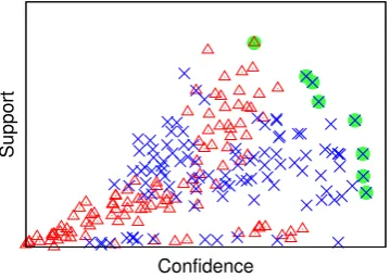
Support

Confidence

Fig. 2: Rx andR∗x. Each point corresponds to a rule inRx. Optimal rules are highlighted.

most valuable ones, since by definition, no other rule excels as much as those rules in the frontier. We denote the rules lying in the Pareto frontier as optimal multi-criteria rules, and given a test instance

x, the corresponding classifierR∗

x is composed of those rules lying in the Pareto frontier.

Figure 2 illustrates this intuition with data obtained from a real example. Each point in the figure corresponds to a rule inRx. It is not evident from the figure if rules pointing to the blue class are better than rules pointing to the red class. However, if we consider only rules lying in the Pareto frontier, it becomes clear that rules pointing to the blue class (which is indeed the correct class) are the ones that excel most. Furthermore, while|Rx|= 210, there are only 8 rules inR∗x, corresponding to a decrease of 96% in terms of model size.

3.3 Employing Additional Frontiers

In some cases, the Pareto frontier is composed of very few rules. As a consequence, the classifierR∗

x may be over-simplified and it may be dangerous to perform predictions since rules inR∗x may be due to noise. Our approach to overcome this problem is to use additional Pareto frontiers. That is, instead of using only the first frontier, we may also exploit subsequent frontiers. This will obviously increase the size of the classifier, since more rules will be included intoR∗

x, reducing the impact of noisy rules. Algorithm 2, which we call PE-LAC (Pareto-Efficient Lazy Associative Classification), shows detailed steps of the entire process of learning interpretable classifiers using Pareto-Efficient rules.

Algorithm 2 PE-LACPareto Efficient Lazy Associative Classification

Require: Training-setD, test instancex, statisticsθto be used in Equation 1, number of frontiersη

1: Rx←induceRules(x,D)

2: Fx← ∅

3: fori= 1to η do

4: Fx←Fx ∪paretoFrontier(Rx−Fx) .apply BNL

5: for allclassyi∈ Y do .notice that Y is the set of all class labels

6: s(x, yi)←

X

r∈Fxyi

θ(r)

7: for allclassyi∈ Y do

8: pˆ(yi|x)← _|Y|s(x,yi)

X

k=1

s(x, yk)

(10)

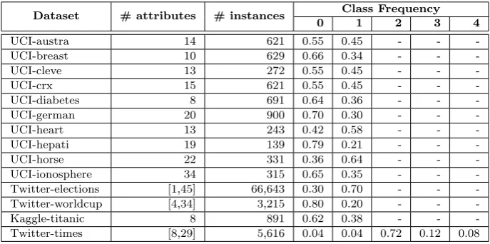
Table II: Datasets.

Dataset # attributes # instances Class Frequency

0 1 2 3 4

UCI-austra 14 621 0.55 0.45 - -

-UCI-breast 10 629 0.66 0.34 - -

-UCI-cleve 13 272 0.55 0.45 - -

-UCI-crx 15 621 0.55 0.45 - -

-UCI-diabetes 8 691 0.64 0.36 - -

-UCI-german 20 900 0.70 0.30 - -

-UCI-heart 13 243 0.42 0.58 - -

-UCI-hepati 19 139 0.79 0.21 - -

-UCI-horse 22 331 0.36 0.64 - -

-UCI-ionosphere 34 315 0.65 0.35 - -

-Twitter-elections [1,45] 66,643 0.30 0.70 - -

-Twitter-worldcup [4,34] 3,215 0.80 0.20 - -

-Kaggle-titanic 8 891 0.62 0.38 - -

-Twitter-times [8,29] 5,616 0.04 0.04 0.72 0.12 0.08

3.4 Computational Complexity

The computational complexity of the original associative classification algorithm, LAC, is given as:

O(|D| × |Y| ×

l

X

k=1 _|_x_|

k

) wherexis a test instance,Y ={y1, y2, . . . , ym} is the set of possible class

labels, andlis the maximum cardinality allowed for the rules (which is bounded by the cardinality of the test instance, that is|x|). As shown in Section 2.5, the BNL algorithm we use to find the Pareto frontier has linear complexity in the best- and average-cases. Thus, in such cases, the complexity of

PE-LAC is given as: O(|D|×|Y|×η×

l

X

k=1 _|_x_|

k

). However, sinceηis a small constant, we conclude that

PE-LAC has essentially the same complexity as LAC. In the worst-case scenario, the BNL algorithm

is quadratic, and thus the complexity of PE-LAC becomes: O(|D| × |Y| ×η×( l

X

k=1 _|_x_|

k

)2).

4. EXPERIMENTAL EVALUATION

In this section we empirically analyze our proposed PE-LAC algorithm in terms of both classification accuracy and model size/interpretability. Our evaluation is based on a direct comparison against the original LAC algorithm [Veloso et al. 2006]. We also employ a baseline classifier based on closed rules, which we call CL-LAC (Closed Lazy Associative Classification), so that we can compare PE-LAC against a strategy based on condensed representations. It is worth mentioning that most of the results can be also compared against other algorithms since we used the same evaluation methodology and the same datasets as Veloso et al. [2006]. Finally, we also evaluate the effectiveness of our proposed strategy when used to filter closed rules, an algorithm we call as CL-PE-LAC (Closed Pareto-Efficient Lazy Associative Classification). We first discuss the evaluation methodology and significance tests, and then we present our results.

4.1 Evaluation Methodology

(11)

about these datasets. Some datasets are structured, and in this case all instances have a fixed number of attributes. Other datasets are obtained from applications that involve textual data (i.e., tweets), and thus instances may have different number of attributes. In all the experiments with the afore-mentioned datasets we used 5-fold cross-validation and the final results of each experiment represent the average of the five runs. Classification accuracy is assessed through the conventional precision, recall andF1 measures. Precisionpis defined as the proportion of correctly classified test instances

in the test-set. Recallris defined as the proportion of correctly classified test instances out of all the instances having the target class. F1 is a combination of precision and recall defined as the harmonic

mean_p2₊pr_r. Macro- and micro-averaging [Yang et al. 2002] were applied toF1to get single performance

values. Micro-F1 essentially corresponds to accuracy, while Macro-F1 is the average of theF1 values

over all classes. Finally, model interpretability is assessed by the number of rules within the classifier.

4.2 Significance Tests

The objective of the PE-LAC algorithm is to decrease the number of rules inRwhile keeping clas-sification accuracy (i.e., Macro- and Micro-F1) approximately the same. In order to check if the

objective was reached we will employ three significance tests for paired-comparison and two group-based hypothesis test. Tests for paired-comparison include: (i) T-Test (parametric), (ii) Wilcoxon (non-parametric), and (iii) Permutation (non-parametric). Group-based hypothesis tests include: (i) ANOVA (parametric), and (ii) Kruskal-Wallis (non-parametric). Additional details about these tests can be found in the work by Wasserman [2010].

We always consider two options: H0is the null-hypothesis, andH1is the alternate hypothesis. In

our case, the null hypotheses that may be accepted or rejected are:

(1) Both LAC and PE-LAC algorithms learn classifiers that achieve the same Micro-F1 values.

(2) Both LAC and PE-LAC algorithms learn classifier that achieve the same Macro-F1values.

(3) Both LAC and PE-LAC algorithms learn classifiers composed of the same number of rules.

The null-hypothesis is only rejected if its probability is very low [Wasserman 2010]. In order to assess the evidence againstH0we use ap-value, which is given asP(T > tobs|Ho), whereT is a given statistics andtobsis the observed value for such statistics (i.e., Macro-F1, Micro-F1, or the number of

rules within the classifier). Typically, the followingp-value’s scale have been used: p < 0.01 implies strong evidence againstH0; 0.01< p≤0.10 indicates weak evidence againstH0; andp >0.10 shows

no evidence againstH0. The case in whichH0is rejected, but is indeed true, is called Type-I error.

Similarly, a Type-II error occurs ifH1 is true butH0 was accepted.

4.3 Results

The first experiment is devoted to evaluate howη impacts classification accuracy. For this experiment we used the UCI datasets, and variedη from 1 to 4 frontiers. Further, due to lack of space we only consider confidence as theθ-statistics used in Equation 1. Micro-F1 numbers may suffer whenη= 1,

indicating that the small number of rules makes the classifier less robust to noise. Clearly, Micro-F1

stabilizes forη values around 3 frontiers. The number of rules, as expected, increases withη. Unless otherwise stated, for now on we will fixη= 3 in all remaining experiments.

Table IV shows Macro- and Micro-F1 numbers, as well as the number of rules within the classifier,

(12)

Table III: PE-LAC: Performance according toη. Objective # fro n tier s ( η ) U CI-au str a UC I-bre ast U CI-clev e UC I-crx U CI-di ab etes U CI-germ a n U CI-hea rt U CI-hep at i UC I-h o rse U CI-ion os ph ere C on

f. Micro-F1 1 0.82 0.95 0.80 0.82 0.69 0.71 0.83 0.82 0.78 0.91

2 0.85 0.96 0.83 0.84 0.75 0.71 0.85 0.83 0.79 0.93 3 0.86 0.97 0.83 0.86 0.78 0.72 0.85 0.83 0.82 0.94 4 0.87 0.97 0.84 0.86 0.78 0.71 0.85 0.84 0.83 0.94

C

on

f. #Rules 1 3 7 3 3 2 5 3 21 15 103

2 5 8 5 6 6 6 5 24 17 107

3 8 9 7 10 9 8 8 27 20 111

4 11 11 10 13 12 10 10 31 23 115

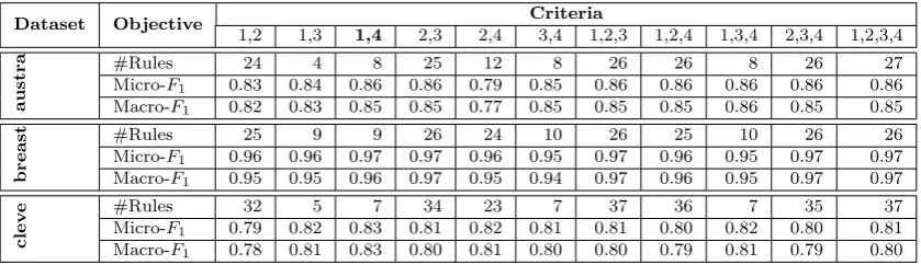
Table IV: PE-LAC: Performance according to criteria (1 =confidence, 2 =support, 3 =added value, 4 =Yules’Q).

Dataset Objective Criteria

1,2 1,3 1,4 2,3 2,4 3,4 1,2,3 1,2,4 1,3,4 2,3,4 1,2,3,4

au

st

ra #Rules 24 4 8 25 12 8 26 26 8 26 27

Micro-F1 0.83 0.84 0.86 0.86 0.79 0.85 0.86 0.86 0.86 0.86 0.86

Macro-F1 0.82 0.83 0.85 0.85 0.77 0.85 0.85 0.85 0.86 0.85 0.85

b

rea

st #Rules 25 9 9 26 24 10 26 25 10 26 26

Micro-F1 0.96 0.96 0.97 0.97 0.96 0.95 0.97 0.96 0.95 0.97 0.97

Macro-F1 0.95 0.95 0.96 0.97 0.95 0.94 0.97 0.96 0.95 0.97 0.97

cl

ev

e #Rules 32 5 7 34 23 7 37 36 7 35 37

Micro-F1 0.79 0.82 0.83 0.81 0.82 0.81 0.81 0.80 0.82 0.80 0.81

Macro-F1 0.78 0.81 0.83 0.80 0.81 0.80 0.80 0.79 0.81 0.79 0.80

of dimensions. Therefore, for now on we employ confidence and Yules’Q as the dimensions of the rule-utility space.

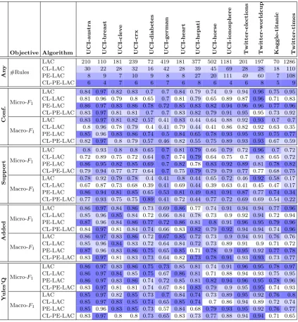
Accuracy numbers as well as model size for LAC and PE-LAC algorithms are shown in Table V. A quick analysis indicates that we have reached our main objective of learning smaller classifiers without hurting classification performance. In most of the cases, the average number of rules withinRx was decreased by two orders of magnitude. For instance, for the UCI-austra dataset the average number of rules decreases from 210 to only 8. Also, in most of the cases, Macro- and Micro-F1numbers obtained

by LAC, CL-LAC, PE-LAC, and CL-PE-LAC are all very similar. In some cases, however, we observe large variations, in many cases favoring PE-LAC.

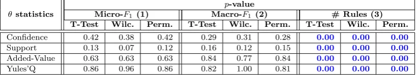
A deeper analysis is necessary in order to verify if the objective of decreasing the number of rules without hurting classification effectiveness was indeed reached. Thus, we apply three paired signifi-cance tests, as shown in Table VI. We evaluate three statistics: Micro-F1, Macro-F1, and the average

number of rules withinRxandR∗x, using the numbers shown in Table V and comparing LAC against PE-LAC under the sameθstatistics (i.e., confidence, support, added-value, or Yules’Q). Clearly, null-hypotheses (1) and (2) are accepted (i.e., both LAC and PE-LAC learn classifiers that achieve the same Micro- and Macro-F1 values), while null-hypothesis (3) is rejected (accepting the alternate

hy-pothesis that LAC and PE-LAC learn classifiers with different number of rules). Although the T-Test is a parametric test, and therefore not the ideal test for small sample sizes, it presentedp-values that are similar to those presented by Wilcoxon and Permutation.

(13)

Table V: Accuracy numbers and model size/interpretability. Darker cells indicate better results.

Objective Algorithm U

CI-au str a U CI-bre ast U CI-clev e U CI-crx UC I-dia b etes U CI-germ a n UC I-hea rt UC I-hep at i UC I-ho rse UC I-ion os ph ere Tw itt er-elec tio ns Tw itt er-w o rld cu p Ka gg le-tit an ic Tw itt er-tim es An y #Rules

LAC 210 110 181 239 72 419 181 377 502 1181 201 197 70 1286

CL-LAC 30 22 28 32 16 42 28 39 45 69 28 28 18 110

PE-LAC 8 9 7 10 9 8 8 27 20 111 49 60 7 108

CL-PE-LAC 6 4 7 6 6 7 6 8 6 4 6 8 5 9

C

on

f.

Micro-F1

LAC 0.84 0.97 0.82 0.83 0.7 0.7 0.84 0.79 0.74 0.9 0.94 0.96 0.75 0.95 CL-LAC 0.81 0.96 0.79 0.8 0.65 0.7 0.81 0.79 0.65 0.89 0.87 0.96 0.71 0.83 PE-LAC 0.86 0.97 0.83 0.86 0.78 0.72 0.85 0.83 0.82 0.94 0.96 0.96 0.77 0.96 CL-PE-LAC 0.83 0.97 0.81 0.81 0.7 0.7 0.83 0.82 0.79 0.91 0.95 0.95 0.73 0.92

Macro-F1

S

up

p

o

rt Micro-F1

Macro-F1

Ad

ded

Micro-F1

Macro-F1

Y

u

les’

Q Micro-F1

Macro-F1

(1) The LAC algorithm shows the same performance numbers (Micro-F1, Macro-F1 or number of

rules), no matter theθ statistics used in Equation 1.

(2) The PE-LAC algorithm shows the same performance numbers (Micro-F1, Macro-F1 or number of

rules), no matter theθ statistics used in Equation 1.

(3) Both LAC and PE-LAC algorithms show the same performance numbers (either in terms of Micro-F1, Macro-F1 or number of rules), no matter theθstatistics used in Equation 1.

The results obtained by the group-based significance tests are shown in Table VII. Considering the Micro-F1, all hypotheses were accepted. Considering the Macro-F1 the hypotheses 1 and 3 were

(14)

Table VI: Paired tests: LAC vs. PE-LAC.

θstatistics

p-value

Micro-F1 (1) Macro-F1 (2) # Rules (3)

T-Test Wilc. Perm. T-Test Wilc. Perm. T-Test Wilc. Perm.

Confidence 0.42 0.38 0.42 0.29 0.31 0.28 0.00 0.00 0.00

Support 0.13 0.07 0.12 0.16 0.12 0.15 0.00 0.00 0.00

Added-Value 0.63 0.63 0.63 0.84 0.77 0.84 0.00 0.00 0.00

Yules’Q 0.86 0.96 0.86 0.82 1.00 0.81 0.00 0.00 0.00

Table VII: Group-based tests: LAC, PE-LAC and both.

Hypothesis

p-value

Micro-F1 Macro-F1 # Rules

ANOVA Kruskal-Wallis ANOVA Kruskal-Wallis ANOVA Kruskal-Wallis

(1) 0.09 0.08 0.01 0.05 1.00 1.00

(2) 0.46 0.46 0.30 0.65 1.00 1.00

(3) 0.10 0.10 0.00 0.14 0.00 0.00

(a) LAC, #Rules=72 (b) PE-LAC, #Rules=4

Fig. 3: Rules generated for one passenger in Titanic (a survivor).

This indicates that theθstatistics used to weight the rules does not impact significantly the results, except by support. The hypothesis that the classifiers built by LAC and PE-LAC have the same size were rejected as expected.

Finally, in order to verify how the classifiers that are built by PE-LAC are much more interpretable than the corresponding classifiers built by LAC, we show in Fig. 3 the classifierRx (built by LAC) and its corresponding counterpartR∗

x (built by PE-LAC) for one passenger in Titanic (a survivor). The rules shown in black indicate the death of the passenger, while the rules shown in blue indicate survival. While it is difficult to grasp some explanation from the classifier built by LAC, we may easily capture the reasons that lead the passenger to survive in the classifier built by PE-LAC−he has one sibling, and was hosted in a cabin.

5. CONCLUSIONS

(15)

unnecessarily complex. Therefore, we propose an alternate classification algorithm, PE-LAC, which learns simpler classifiers, that are highly readable. The proposed PE-LAC algorithm evaluates each rule by taking into account multiple criteria simultaneously, such as: confidence, support, added-value, and Yules’Q. These criteria correspond to the dimensions of a rule-utility space. Then, we employ a central concept in Economics, known as Pareto Efficiency, in order to filter rules that excel in at least one dimension in the rule-utility space. We showed, using benchmark data as well as data obtained from recent application scenarios, that both LAC and PE-LAC are similar in terms of classification effectiveness, but PE-LAC learns classifiers that are orders of magnitude smaller/simpler than the classifiers built by LAC. This conclusion is supported by a number of paired and group-based significance tests. Also, we compared PE-LAC against CL-LAC, a filtering strategy which relies on closed rules, and the results show that: (i) PE-LAC builds smaller classifiers than the ones produced by CL-LAC, but in this case classification performance is similar, and (ii) CL-LAC builds smaller classifiers than the ones produced by PE-LAC, but in this case the classifiers produced by PE-LAC are more accurate than the ones produced by CL-LAC. An alternate strategy, which we call CL-PE-LAC, filters closed rules and showed to be competitive with PE-CL-PE-LAC, but in some cases the number of rules becomes excessively small compromising classification performance.

REFERENCES

Agrawal, R.,Imielinski, T.,and Swami, A. Mining Association Rules between Sets of Items in Large Databases.

InProceedings of the ACM SIGMOD International Conference on Management of Data. Washington, USA, pp.

207–216, 1993.

Bache, K. and Lichman, M.UCI Machine Learning Repository. http://archive.ics.uci.edu/ml, 2013.

Blumer, A.,Ehrenfeucht, A.,Haussler, D., and Warmuth, M. Occam’s Razor. Information Processing Let-ters24 (6): 377–380, 1987.

B¨orzs¨onyi, S.,Kossmann, D.,and Stocker, K. The Skyline Operator. InProceedings of the IEEE International Conference on Data Engineering. Washington, DC, USA, pp. 421–430, 2001.

Breiman, L.,Friedman, J.,Olshen, R.,and Stone, C. Classification and Regression Trees. Wadsworth, 1984.

Chipman, H.,George, E.,and McCulloch, R. Bayesian Treed Models.Machine Learning 48 (1-3): 299–320, 2002.

Corne, D.,Knowles, J.,and Oates, M. The Pareto Envelope-Based Selection Algorithm for Multi-objective Opti-misation. InProceedings of Parallel Problem Solving from Nature. Dortmund, Germany, pp. 839–848, 2000.

Cortes, C. and Vapnik, V. Support-Vector Networks. Machine Learning20 (3): 273–297, 1995.

Cover, T. and Hart, P. Nearest Neighbor Patter Classification. IEEE Transactionson Information Theory13 (1): 21–27, 1967.

Domingos, P. The Role of Occam’s Razor in Knowledge Discovery. Data Mining and Knowledge Discovery 3 (4): 409–425, 1999.

Domingos, P. and Pazzani, M. On the Optimality of the Simple Bayesian Classifier under Zero-One Loss. Machine

Learning29 (2-3): 103–130, 1997.

Fidelis, M.,Lopes, H.,and Freitas, A. Discovering Comprehensible Classification Rules with a Genetic Algorithm. InProceedings of the IEEE Congress on Evolutionary Computation. California, USA, pp. 805–810, 2000.

Gehrke, J.,Ganti, V.,Ramakrishnan, R.,and Loh, W.Boat-Optimistic Decision Tree Construction. InProceedings of the ACM SIGMOD International Conference on Management of Data Conference. Philadelphia, USA, pp. 169– 180, 1999.

Godfrey, P.,Shipley, R.,and Gryz, J. Algorithms and Analyses for Maximal Vector Computation. The VLDB Journal16 (1): 5–28, 2007.

Goldbloom, A. Titanic: machine learning from disaster. http://www.kaggle.com, 2012.

Gouda, K. and Zaki, M. GenMax: an efficient algorithm for mining maximal frequent itemsets. Data Mining and

Knowledge Discovery11 (3): 223–242, 2005.

Jakulin, A.,Mozina, M.,Demsar, J., Bratko, I.,and Zupan, B. Nomograms For Visualizing Support Vector Machines. InProceedings of the ACM SIGKDD International Conference on Knowledge Discovery and Data Mining. Chicago, USA, pp. 108–117, 2005.

Joachims, T. Training Linear SVMs in Linear Time. InProceedings of the ACM SIGKDD International Conference on Knowledge Discovery and Data Mining. Philadelphia, USA, pp. 217–226, 2006.

Lattimore, T. and Hutter, M. No Free Lunch versus Occam’s Razor in Supervised Learning. Computing Research Repositoryvol. abs/1111.3846, 2011.

(16)

Letham, B., Rudin, C., McCormick, T.,and Madigan, D. Building Interpretable Classifiers with Rules Using Bayesian Analysis. Department of Statistics Technical Report tr609, University of Washington, 2012.

Li, W.,Han, J.,and Pei, J. CMAR: accurate and efficient classification based on multiple class-association rules. In

Proceedings of the IEEE International Conference on Data Mining. Washington, USA, pp. 369–376, 2001.

Liu, B.,Hsu, W.,and Ma, Y. Integrating Classification and Association Rule Mining. In Proceedings of the ACM SIGKDD International Conference on Knowledge Discovery and Data Mining. New York, USA, pp. 80–86, 1998.

Lowd, D. and Domingos, P. Naive Bayes Models for Probability Estimation. InProceedings of the International Conference on Machine Learning. Los Angeles, USA, pp. 529–536, 2005.

Lucchese, C.,Orlando, S.,and Perego, R. DCI Closed: a fast and memory efficient algorithm to mine frequent closed itemsets. InProceedings of the ICDM Workshop on Frequent Itemset Mining Implementations. Brighton, UK, 2004.

Lucchese, C.,Orlando, S.,and Perego, R.Mining Top-K Patterns from Binary Datasets in Presence of Noise. In Proceedings of the SIAM International Conference on Data Mining. Columbus, USA, pp. 165–176, 2010.

Madigan, D., Mosurski, K., and Almond, R. Explanation in Belief Networks. Journal of Computational and

Graphical Statisticsvol. 160, pp. 181, 1997.

Marchand, M. and Sokolova, M. Learning with Decision Lists of Data-Dependent Features. Journal of Machine Learning Researchvol. 6, pp. 427–451, 2005.

McCormick, T.,Rudin, C.,and Madigan, D.Bayesian Hierarchical Rule Modeling for Predicting Medical Conditions. The Annals of Applied Statisticsvol. 6, pp. 652–668, 2012.

Menezes, G.,Almeida, J.,Bel´em, F.,Gon¸calves, M.,Lacerda, A.,de Moura, E.,Pappa, G.,Veloso, A.,and Ziviani, N.Demand-Driven Tag Recommendation. InProceedings of the European Conference on Machine Learning

and Principles and Practice of Knowledge Discovery in Databases. Berlin, Heidelberg, pp. 402–417, 2010.

Mozina, M.,Demsar, J.,Kattan, M.,and Zupan, B. Nomograms for Visualization of Naive Bayesian Classifier. InProceedings of the ACM SIGKDD International Conference on Knowledge Discovery and Data Mining. Seattle, USA, pp. 337–348, 2004.

Mramor, M.,Leban, G.,Demsar, J.,and Zupan, B. Visualization-Based Cancer Microarray Data Classification Analysis.Bioinformatics23 (16): 2147–2154, 2007.

Pak, A. and Paroubek, P. Twitter as a Corpus for Sentiment Analysis and Opinion Mining. InProceedings of The International Conference on Language Resources and Evaluation. Valletta, Malta, pp. 1320–1326, 2010.

Palda, F. Pareto’s Republic and the new Science of Peace. Cooper-Wolfling, 2011.

Piatetsky-Shapiro, G.Discovery, Analysis and Presentation of Strong Rules. InKnowledge Discovery in Databases.

AAAI Press, Cambridge, USA, pp. 229–248, 1991.

Quinlan, J. C4.5: Programs for Machine Learning. Morgan Kaufmann, San Francisco, USA, 1993.

Rivest, R. Learning Decision Lists.Machine Learning2 (3): 229–246, 1987.

Rudin, C.,Letham, B.,Salleb-Aouissi, A.,Kogan, E.,and Madigan, D.Sequential Event Prediction with Associ-ation Rules.Journal of Machine Learning Research - Proceedings Trackvol. 19, pp. 615–634, 2011.

Santana, I.,Gomide, J.,Veloso, A.,Jr., W. M.,and Ferreira, R. Effective Sentiment Stream Analysis with Self-Augmenting Training and Demand-Driven Projection. InProceedings of the International ACM SIGIR Conference on Research & Development of Information Retrieval. Beijing, China, pp. 475–484, 2011.

Tan, P.,Kumar, V.,and Srivastava, J. Selecting the Right Interestingness Measure for Association Patterns. In Proceedings of the ACM SIGKDD International Conference on Knowledge Discovery and Data Mining. Edmonton, Canada, pp. 32–41, 2002.

Veloso, A. and Meira Jr., W.Demand-Driven Associative Classification. Springer, 2011.

Veloso, A.,Meira Jr., W.,and Zaki, M.Lazy Associative Classification. InProceedings of the IEEE International Conference on Data Mining. Hong Kong, China, pp. 645–654, 2006.

Vreeken, J.,van Leeuwen, M.,and Siebes, A.Krimp: mining itemsets that compress.Data Mining and Knowledge

Discovery23 (1): 169–214, 2011.

Wasserman, L.All of Statistics: a concise course in statistical inference. Springer, 2010.

Yang, Y.,Slattery, S.,and Ghani, R. A Study of Approaches to Hypertext Categorization. Journal of Intelligent Information Systems18 (2-3): 219–241, 2002.

Yin, X. and Han, J.CPAR: classification based on predictive association rules. InProceedings of the SIAM Interna-tional Conference on Data Mining. San Francisco, USA, pp. 331–335, 2003.