A STOCHASTIC PARAMETER REGRESSION APPROACH FOR TIME-VARYING RELATIONSHIP BETWEEN GOLD AND SILVER PRICES

(1)

APPROACH FOR TIME-VARYING RELATIONSHIP

BETWEEN GOLD AND SILVER PRICES

by

Birsen Canan-McGlone

A thesis

submitted in partial fulfillment of the requirements for the degree of

Master of Science in Mathematics Boise State University

(2)

(3)

DEFENSE COMMITTEE AND FINAL READING APPROVALS

of the thesis submitted by

Thesis Title: A Stochastic Parameter Regression Approach for Time-Varying Rela-tionship between Gold and Silver Prices

Date of Final Oral Examination: 11 May 2012

The following individuals read and discussed the thesis submitted by student Birsen Canan-McGlone, and they evaluated her presentation and response to questions during the final oral examination. They found that the student passed the final oral examination.

Jaechoul Lee, Ph.D. Chair, Supervisory Committee

Leming Qu, Ph.D. Member, Supervisory Committee

Jodi Mead, Ph.D. Member, Supervisory Committee

(4)

The author wishes to express her gratitude to her advisor, Dr. Jaechoul Lee, who offered invaluable assistance, support, and guidance.

She also wishes to express her love and gratitude to her beloved husband, Dave McGlone for his understanding and endless support during her studies.

(5)

In this thesis, we studied the gold and silver relationship using stochastic-parameter regression models. We formulated their time-varying relationship as a state-space model and used the Kalman filter algorithm to estimate the stochastic regression parameters for gold and silver prices. The data set used in this thesis covers 31 years using the London fix prices between January 1969 and December 2000. The start date was selected as the first full year silver prices were included in the London fix prices. Our stochastic parameter regression model explained well the time-varying relationship between gold and silver prices. As a special case of the stochastic param-eter regression model, we also fitted the random walk, the random walk with drift model and random coefficient model. The random walk with drift model appeared to have the closest fit with 12-month forecast errors minimal among those four models considered in this thesis.

(6)

ABSTRACT . . . iv

LIST OF TABLES . . . vii

LIST OF FIGURES . . . viii

1 INTRODUCTION . . . 1

2 BACKGROUND . . . 4

2.1 Gold and Silver . . . 4

2.1.1 A Brief History of Gold and Silver . . . 4

2.1.2 Industrial Uses of Gold and Silver . . . 8

2.2 Regression Models with Stochastic Parameters . . . 10

2.2.1 The State-Space Model . . . 10

2.2.2 Kalman Filter . . . 12

2.2.3 Estimation of Fixed Coefficients: Maximum Likelihood Estimation15 2.2.4 Prediction of Future Values . . . 18

2.2.5 Estimation of the Sample Period Stochastic Parameter . . . 19

2.2.6 Summary . . . 21

3 STOCHASTIC PARAMETER MODEL FOR GOLD AND SILVER22 3.1 Random Coefficient Model . . . 24

3.2 First-Order Autoregression Coefficient Model . . . 26

(7)

3.4 random walk without Drift Model . . . 35

3.5 Prediction . . . 39

4 CONCLUSIONS . . . 43

REFERENCES . . . 45

A R-PROGRAMS . . . 48

(8)

3.1 Fixed Parameters of Random Coefficient Model . . . 24

3.2 Fixed parameters of first-order autoregression Coefficient model . . . 27

3.3 Fixed Parameters of random walk with Drift Model . . . 31

3.4 Fixed Parameters of random walk Model . . . 35

3.5 (SSPE) and (SAPE) of four models’ 2001, 12 months predictions . . . 41

(9)

3.1 London Fix monthly average gold (black) and silver (blue) prices be-tween January 1969 and December 2000. . . 23 3.2 Random coefficient model’s estimates for one step-ahead prediction

coefficients βt is black, estimates for smoothed βt is blue. These

pa-rameters represents the gold/silver ratio. . . 25 3.3 Gold prices (blue) random coefficient regression model fit (red) and

residuals. . . 26 3.4 First-order autoregression Coefficient model’s estimates for one

step-ahead prediction coefficientβt and its ACF and PACF. . . 28

3.5 Gold prices (black) first-order autoregression Coefficient model fit(red) and its residuals. . . 29 3.6 First-order autoregression Coefficient model’s estimates for one

step-ahead prediction coefficient βt is black, estimates for smoothed βt is

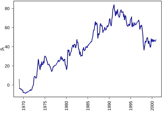
blue. These parameters represents the gold silver ratio. . . 30 3.7 Random walk with drift model’s estimates for one step-ahead

predic-tion coefficients βt is black and smoothed βt is blue. . . 32

3.8 Random walk with drift model’s estimates of one step-ahead prediction coefficients βt and its ACF and PACF. . . 33

3.9 Gold prices (black) random walk with drift model fit(red) and residuals. 34

(10)

diction’s βt is black, estimates for smoothed βt is blue. . . 36

3.11 random walk Without Drift model’s estimates of one step-ahead pre-diction coefficientsβt and its ACF and PACF. . . 37

3.12 Gold prices (black) random walk without drift model fit (red) and residuals. . . 38 3.13 Gold, silver prices and model fit of gold for four models: AR(1)

co-efficient model (ARR), random walk with drift (RWD), random walk (RD), and random coefficient (RC) . . . 40 3.14 βt of one step ahead predictions of four models between January of

1969 and December of 2000 . . . 41 3.15 Prediction for random coefficient (RC), random walk (RW), random

walk with drift (RWD), AR(1) coefficient model (FS) between January of 1969 and December of 2000 . . . 42

(11)

CHAPTER 1 INTRODUCTION

Throughout history, gold and silver have been used as currency. In the last two centuries, governments of many countries backed their printed money with gold or silver, or both. This is called gold or silver, or bi-metallic standard. However, during the second half of the last century, most countries abandoned gold and silver standards and stopped using gold and silver in their currencies. Since then, gold and silver have become commodities traded on general commodities markets. Still, gold and silver hold a special place in the minds of investors who would like a hedge against inflation. In addition, given recent changing economic conditions along with a growing distrust of the monetary system, many states in the U.S. have chosen to legalize gold and silver as currency: Idaho, Utah, and Washington are a few of them.

From an investment point of view, there are additional incentives for investors in gold and silver. Both are used in the jewelry markets. Recently demand has increased for silver in industrial uses (such as the medical field, food preparation, and contaminant remediation). Gold has similar industrial uses, but there is a significant difference in their prices. Gold is extensively used in electronics manufacturing, more than silver, because it has good electrical properties and is not prone to oxidation as silver is.

(12)

between gold and silver prices. Chan and Mountain [2] analyzed weekly data and interest rates for the early 1980s and developed time series models to test for the causality between the price of gold, the price of silver and interest rates by using an arbitrage model that takes advantage of a price difference between two or more markets. They concluded that there is a causal feedback relationship between the price of gold and the price of silver.

Akgiray et al. [1] investigated daily returns for gold and silver for the period be-tween 1975 and 1986, where the returns were the natural logarithms of the ratio of the two successive daily spot prices. They found no forecastibility in the way of returns. Because the variance of the returns was not constant, they modeled this variance as a GARCH process (Generalized Auto Regression Conditional Heteroscedasticity).

Escribano and Granger [4] focused on gold and silver price during 1971-1990. They found that cointegration occurred during certain periods, especially during the bubble period from September of 1979 to March of 1980. To establish a linear relationship for the entire data set between gold and silver prices, they used dummy variables for intercept terms. They claimed their model performed better than the random walk model for available data. However, their model failed for the out-of-sample predictability. They concluded that a dependency between gold and silver prices decreased after 1990, indicating that the two markets were separating.

(13)

functions to fit the marginal and joint probability density function (pdf), resulting in a better model. They found that silver returns were higher than gold in both markets during this period.

The analysis performed in this work is different from previous works, because we studied the historical relationship between gold and silver prices and the future direction of their relationship. We analyzed the relationship of gold and silver London Fix prices between 1969 and 2001 using a state-space model. We investigated this relationship using four models: first order autoregression coefficient, random walk with drift, random walk without drift, and random coefficient models. The results of these analysis are compared based on their forecasting ability.

(14)

CHAPTER 2 BACKGROUND

2.1 Gold and Silver

2.1.1 A Brief History of Gold and Silver

Many historical facts about gold and silver are likely of not much use to the analysis in this work. However, they provide insight on the close historical relationship between gold and silver. As far back as 3100 B.C., there is evidence of a gold/silver value ratio set by the founder of the first Egyptian dynasty as 10/25 [12]. This is the earliest set relationship between gold and silver. In 1700, Sir Isaac Newton in his capacity of Master of the Mint, fixes the price of gold in Britain at 84 shilling, 11 pence per troy ounce. During this time, the royal commission recalls all gold currencies and fixes the gold silver ratio as 16/1. This legal ratio lasted over 200 years [12]. Throughout history, gold and silver have been used as currency and their prices were controlled by the governments. Starting around the second half of the 20th century, governments of the world started to loosen their control on the price of gold and silver.

We found it useful to provide a list of some of the more significant historical facts and dates that is pertinent to our work [10], [12]:

• 1961: owning gold is forbidden for Americans abroad as well as at home. At the

(15)

West Germany, United Kingdom, and United States form the London Gold pool and agree to buy and sell gold at $35.0875 per ounce.

• 1964: The U.S. is taken off the silver standard. The issuance of silver certificates

is stopped and the redemption of them is suspended after 1968.

• 1968: Governors of the central banks in the gold pool announce they will no longer buy gold and sell gold in the private market. A two-tier pricing system starts: Official transactions between monetary authorities are to be conducted at an unchanged price $35 per troy ounce, and other transactions are to be conducted at a fluctuating free-market price. Gold backing of Federal Reserve notes is eliminated. In technology side, Intel introduces a microchip with 1024 transistors interconnected with gold circuit. More new uses of gold in electronics and medical fields are being discovered.

• 1969: The U.S. Mint presses its last silver coin.

• 1971: The U.S. terminates all gold sales or purchases, thereby ending conversion

of foreign officially held dollars into gold. Under the Smithsonian agreement, the U.S. dollar is devalued by raising the value of gold to $38 per troy ounce.

• 1973: The U.S. devalues the dollar again and announces it will raise the official

dollar price of gold to $42.22 per troy ounce. All currencies allowed to freely float without regard to gold prices. In June, the gold price rises more than $120 in London market. Japan lifts the prohibition on import of gold.

(16)

• 1975: U.S. treasury and IMF start selling its gold. Trading in gold for future

delivery begins on New York’s Commodity exchange and on Chicago’s Interna-tional Monetary Market and Board of Trade. The Krugerrand is launched on to U.S. markets.

• 1978: The IMF and the U.S. abolish the official price of gold. Member

govern-ments can buy or sell gold in private markets. The U.S. Congress passes the American Arts Gold Medallion Act, representing the first official issue of a gold piece for sale to individuals. Japan lifts its ban on gold exports.

• 1979: Canada introduces 1 ounce Maple leaf.

• 1979/June-1980/March silver bubble caused by the Hunt brothers of Texas. This resulted substantial changes in market trading rules [5].

• 1980: IMF sells 1/3 of its gold to IMF members. The U.S. sells 15.8 million

troy ounce of gold to strengthen its trade balance. A weakening U.S. dollars raises interest in gold, assumed to be aided by historic events such as the U.S. recognition of Communist China, events in Iran and Sino-Vietnam border disturbances. Gold reaches historic high of $870 and drops to $591 at the year end.

• 1981: The U.S Treasury forms a gold commission to assess and make

recom-mendations with regard to the policy of the U.S. government concerning the role of gold in domestic and international monetary system. Gold is used in coating of the first space shuttle’s liquid impellers.

• 1986: The American Eagle gold Bullion coin is introduced by the U.S. Mint.

(17)

coated compact discs are introduced, which provides perfect reflective surfaces, eliminates pinholes and eliminating all possibility of oxidative deterioration of the surfaces.

• 1987: British Royal Mint introduces the Britannia Gold Bullion coin. World stock market crashes on October; in commodities market shows increase in gold activity. The world gold council is established to sustain and develop demand for the end uses of gold.

• 1988: Japan purchases huge amounts of gold to mint a commemorative gold

coin to celebrate 60th anniversary of Emperor Hirohito’s reign.

• 1989: Austria introduces the Philharmonic bullion coin.

• 1993: Germany lifts its tax restriction on financial gold, causing a increase in

private demand of gold. India and Turkey free their gold markets.

• 1994: Russia formally establishes gold market.

• 1996: The Mars Global surveyor is launched with an on board gold coated

parabolic telescope-mirror.

• 1997: The U.S. Congress passes a bill allowing U.S. individual retirement

account holders to buy gold bullion coins and bars for their accounts as long as they are 99.5% purity of gold.

• 1999: The Euro is introduced backed by a new European Central Bank holding

15% of its reserves in gold.

(18)

The post-1968 data is necessary to interpret the shock to the price of gold and silver. For that reason, we will be referring to these points in the later sections while interpreting our model results.

2.1.2 Industrial Uses of Gold and Silver

Throughout history, gold and silver were mainly used as currency and jewelry. However, recent changes in their status as currency do not diminish their value. They are two of the best conductors of electricity and heat, most reflective of all metals, are powerful anti-bacterial agents, and are easily worked since they are malleable and ductile. These properties make them two of the most sought out and revered metals [13], [11].

The most important industrial use of gold is in electronics manufacturing. A small amount of gold is used in almost every electronic device. Silver is the best conductor of electricity so it finds many uses in electronics as well. Even though gold is a number-3 conductor. One of gold’s advantages is that it does not oxidize. Chemical reactions use silver as a catalyst. More than 700 tons of silver are used each year to produce ethylene oxide and formaldehyde, both of which are essential to the plastics industry. Silver oxide-zinc batteries are being used in portable electronic devices, like watches, cameras, and other small electronic devices. As one of the most reflective metals next to gold, silver is used in specialized optical devices, automobile windshields, and both commercial and household mirrors [11], [13].

(19)

silver kept the freshness and prevented spoilage of oil, wine, and water. Wealthy ancient Greeks and Romans stored these in silver jugs. Silver compound shows a toxic effect on bacteria, viruses, algae, and fungi. Silver also has wide range of use in health and medical applications. These include dressing and ointments for burns and wounds, anti-bacterial pharmaceutical, and coating of surgical instruments. Silver is being used for water purification and treatment containing radioactive and biological contaminants [11]. Even though gold has similar antibacterial properties, using gold instead of silver would be a very expensive alternative. Recently clothing is being manufactured with silver-impregnated fabric to kill bacteria and fungi in order to reduce disease and odor. Recent research shows that silver also promotes the production of new cell growth, speeding the healing process of wounds and bones [11].

Gold is too expensive to use randomly. It is used purposefully and only when less expensive alternatives cannot be found. Most of the ways gold is used in industry have been developed only during the past three decades. This trend will most likely continue. As the use of sophisticated electronics increase, the use of industrial gold will increase. The need for silver is also expected to keep increasing [11].

(20)

2.2 Regression Models with Stochastic Parameters

2.2.1 The State-Space Model

The state-space model or dynamic linear model (DLM), in its basic form, employs an order one autoregression (AR(1)) as the state equation:

βt−β = Φ(βt−1−β) +at (2.1)

where the state equation determines the rule for the generation of the K ×1 state vector βt from the past K ×1 state βt−1, for time points t = 1, . . . , n. The K ×1

stochastic parameter βt has constant mean β, and Φ is a K ×K matrix of fixed

parameters. We assume at are K×1 independent and identically distributed (IID),

zero mean normal vectors withK×Kcovariance matrixQ. In the state equation (2.1), we assume the process starts with initial vector β0 that has mean µ0 and K ×K

covariance matrix Σ0 (or σ0 for univariate case). The state-space model adds an

additional component to the regression model in assuming we do not observe the state vector βt directly, but only a linear transformed version of it with noise added:

yt =α+zt0βt+et (2.2)

wherezt isq×K measurement or observations vector, yt are q×1 observation vector

in (2.2) and et are q×1 IID, zero mean normal vectors with q×q covariance matrix

R, and α is an intercept term. The model in (2.2) is called measurement, or space equation.

(21)

filter may be applied and this in turn leads to algorithms for prediction and smoothing. The Kalman filter is a recursive procedure for computing the optimal estimator of the state vector at timet based on all the information available at timet, [8], [3], [6]. The current values of the state vector is of prime interest and Kalman filter enables the estimate of the state vector to be continually updated as new observations (or information) become available. The state vector may not have an economic interpretation but in cases where it does, it is more appropriate to estimate its value at a particular point in time using all the information in the sample, not just a part of it.

In econometrics, the Kalman filter became important, due to its forecasting ability. Another reason for the popularity of the Kalman filter is that when the disturbances and the initial state vector are normally distributed, it enables the likelihood function to be calculated via what is known as the prediction error decomposition. This opens the way for the estimation of any unknown parameters in the model. It also provides the basis for statistical testing and model specification.

The derivation of the Kalman filter given below is based on the assumption that the disturbances and initial state vectors are normally distributed. A standard result on the multivariate normal distribution is then used to show how it is possible to recursively calculate the distribution ofβt, conditional on the information set at time

t for all t from 1 to T. These conditional distributions are themselves normal and thus are completely specified by their means and covariance matrix.

After having derived the Kalman filter, it is shown that the mean of the conditional distribution ofβtis an optimal estimator ofβtin the sense that it minimizes the mean

(22)

state vector. However, it is still an optimal estimator in the sense that it minimizes the MSE within the class of all linear estimators [8].

2.2.2 Kalman Filter

Let us assume we haveT observations ofy1, . . . yT on a dependent variable, and

cor-respondingly, observations Ai1, . . . AiT where i = 1, . . . , K. Assuming linear relation

between yt and Ait, we can write:

yt =β1tA1t+β2tA2t+· · ·+βKtAKt+et (2.3)

or equivalently,

yt=α+Atβt+et (2.4)

βt−β = Φ(βt−1−β) +at (2.5)

where At = (A1t. . . AKt)0, We assume at and et are independent white noise and are

uncorrelated. Ait are either fixed observations or random variables, independent of

both at and et. The model described by (2.4) and (2.5) is a special case of a general

class of models called state-space models. This model has been extensively presented in [3]. We will use this state-space model in Chapter 3 as a base model for analyzing silver and gold prices. Specifically, the state-space model equations are rearranged to obtain a random walk and random coefficient model.

In this work, we assume that the joint distribution ofytandβtfor giveny1, . . . , yt−1

(23)

ex-pected value and covariance matrix of the stochastic parameterβt, given information

available at time t. At this point, it would be useful to introduce some further notation.

First, consider the distribution ofβt, given information up to timet−1,y1, . . . , yt−1.

We will use β(t|n) to denote expected value (mean) of this distribution, and P(t|n) to denote its K×K covariance matrix. These can be written as

β(t|n) =E[βt|y1. . . yn];P(t|n) =V ar[βt|y1. . . yn].

We also need to consider the distribution of yt, given information up to and

including time t−1. The mean and variance of this distribution can be written as

y(t|n) = E[yt|y1. . . yn];ht =V ar[yt|y1. . . yn].

We already assumed that βt and yt are normally distributed. Now it is necessary

to find the joint distribution of βt and yt given the observation y1, . . . , yt−1. As a

consequence of the normality assumption, it follows that this joint distribution will be multivariate normal. Using the well-known results on the multivariate normal distribution, we can find the mean and the covariance of this distribution. For further details, see Appendix of [8] and [6].

Derivation of the expected value and covariance matrix ofβtandytgiveny1, . . . , yt−1,

can be found in [6] and [8]. These expected values and covariance matrices comprise the Kalman algorithm. Here, we will only list the following pertinent equations of the Kalman algorithm.

β(t|t−1) = Φβ(t−1|t−1) + (I+ Φ)β (2.6)

P(t|t−1) = ΦP(t−1|t−1)Φ0+Q (2.7)

(24)

β(t|t) = Φβ(t−1|t−1) + (I−Φ)β+P(t|t−1)Ath−t1[yt−A0tβ(t|t−1)] (2.9)

P(t|t) = P(t|t−1)−P(t|t−1)Ath−t1A 0

tP(t|t−1) (2.10)

To find expected values for βt and yt, given all the previous values of yt, we use

Kalman algorithm equations (2.6)-(2.10). Here β(t|t−1) is the conditional expected value of βt, P is the conditional covariance matrix of βt, and ht is the covariance of

yt.

The Kalman algorithm provides a computationally efficient framework to solve the problem of estimating the fixed parameters (Φ, α, β, Q, R) of the regression model and forecasting the future values of yt. These parameters will be estimated by the

maximum likelihood method (ML) utilizing Newton-Raphson method.

In order to utilize the Kalman filter algorithm, initial values, namely β(0|0) and P(0|0), are needed. These are mean and covariance of β0 given no previous

observation. These starting values can be substituted into the Kalman filter equa-tions (2.6)-(2.10) to compute recursively the means and the variances of the dependent variables and stochastic parameters in any time period, given information available in the previous period and the fixed coefficient of the model.

(25)

in our model.

2.2.3 Estimation of Fixed Coefficients: Maximum Likelihood Estimation

Let Θ = (µ0,Σ0,Φ, α, β, Q, R) represent the vector of the unknown parameters in

model (2.1) and (2.2) containing the initial mean and covariance of β0, denoted by

µ0, Σ0, the transition matrix Φ, and Q and R are the state and space observation

covariance matrix, respectively. The likelihood function can be evaluated under the initial assumption that the initial β0 is normal with mean µ0, and variance Σ0, and

errorsa1, . . . , aT, ande1, . . . , eT are jointly normal and{at}and{et}are uncorrelated.

The likelihood is computed using the innovations 1, . . . , t defined as t = yt−

Atβ(t|t−1)−α. The innovation form of the likelihood is given in Shumway and

Stoffer [8], Newbold and Bos [6], and references therein.

Given observations taken over t time points, we want to obtain estimates of the fixed parameters. In doing so, we need to derive the likelihood function which is the joint distribution of y1, . . . , yt as a function of fixed parameters of our model. The

joint probability density function of y1, . . . , yt can be expressed as the product of the

conditional density of yt given y1, . . . , yt−1, that is f(y1, . . . , yt) = f(y1)·f(y2|y1)·

f(y3|y1, y2). . . f(yt|y1, . . . , yt−1). We also know that the distribution of yt given all

the observations y1, . . . , yt−1 is normal with expected value given by y(t|t − 1) =

α+A0_tβ(t|t−1) and covarianceht given asht =A0tP(t|t−1)At+σ2. The conditional

probability density function, then, can be written as:

f(yt|y1, y2, . . . , yt−1) =

1 √

2πht

e−(yt−A0_tβ(t|t−1))2/2ht _(2.11)

(26)

function, that is the joint distribution function, as

L= (2π)−n/2

n Y

t=1

h−_t1/2e−Pnt=1(yt−A

0

tβ(t|t−1))2/(2ht) _(2.12)

Taking the natural logarithms yields the log-likelihood function, which is actually easier to work with than the likelihood function, as follows:

lnL= n

2ln(2π) + 1 2

n X

t=1

lnht+ n X

t=1

yt−A0tβ(t|t−1))2

ht

!

(2.13)

The log-likelihood equation (2.13) provides the function that must be maximized to obtain maximum likelihood estimates of the fixed parameters. In reality, it is taken as −lnL, and it must be minimized. The equation (2.13) includes the observationyt

and At, along with conditional variance ht of the dependent variable and conditional

expectation of stochastic parameter β(t|t−1). The conditional variance ht and the

expectationβ(t|t−1) are functions of the fixed parameters defined in the Kalman filter algorithm. We use the Kalman algorithm to calculate them recursively for the given fixed parameters. To find the fixed parameters, we need to solve the log-likelihood function.

Because htand β(t|t−1) are complicated functions, it is not possible to solve this

log-likelihood function analytically. Therefore, numerical optimization algorithms must be employed with respect to fixed parameters of the state-space model. Today, most statistical softwares include optimization packages. In this thesis, we used

(27)

method. This method requires only the derivatives of the function to be minimized. Then, the derivatives are evaluated numerically.

Another advantage of the numerical maximization of the likelihood function is that it provides the standard errors associated with estimators along with point estimates of the fixed parameters. This is accomplished through the information matrix. Let Θ be the vector of all the fixed parameters andLbe the likelihood function, then the information matrix is the expectation of the second derivatives of lnL with respect to each parameters:

I(Θ) = ∂

2_ln_L

∂Θ∂Θ0 (2.14)

It can be assumed that this approximation is valid for large sample sizes. Then, the covariance matrixV(Θ) of the maximum likelihood estimators of Θ isV(Θ) =I(Θ)−1_.

Newton-Raphson Estimation Procedure

The steps involved in performing a Newton-Raphson estimation procedure are as follows.

1. Choose: Initial values of mean and variance of βt: µ0,Σ0, and initial fixed

parameters of state-space model: Θ(0) _{= (Φ}_{, α, β, Q, R}₎

2. Run the Kalman filter algorithm (2.6)-(2.10) to obtain a set of error values

(0)_t =yt−α−At·βt and covariance Σ (0)

t ; t= 1, . . . , n.

3. Run Newton-Raphson algorithm with −lnLY(Θ) as the criterion function to

(28)

4. At the iteration j, repeat Step 2 to obtain new set of (_tj)=yt−α−At·βt and

Σ(_tj). Then, repeat Step 3 to obtain a new set of Θ(j)_{, stop when MLE stabilize;}

for example, stop when the values of Θ(j+1) differ from Θ(j), or whenLY(Θ(j+1))

differs from LY(Θ(j)), by some pre-determined small amount [8].

The only time inputs in this procedure are for the initial values for Θ = (µ0,Σ0,Φ, α, β, Q, R).

This is a trial and error process, and one can only make educated guesses for these inputs. However, this can be a very arduous process. In this study, we assumed linear relation between yt and At, in that the intercept and slope provided initial values for

α and µ0. We also assumed initial β is to be equal to µ0. For the rest of the fixed

parameters, we made educated guess. The algorithm we used in this study can be found in A.

2.2.4 Prediction of Future Values

We start with set of observed data, namely yt and Ait. Both data set cover the

same period in time. From these data, we find the fixed parameters of the state-space model and stochastic regression coefficients. Then, we would be able to describe the relationship between these two variables.

The primary aim of the state-space model approach is to produce estimators for the underlying unobserved signal βt. Then, we will assumed that yt are generated by

this stochastic regression model. We will further assume that this model continues to hold true in the future.

The problem we encounter here is that, to predict future values of y, we have to have the foreknowledge ofAi due to the fact that Ai is the independent variable and

(29)

the values that the dependent variable will take, given specific future values of the independent variableAit.

The stochastic parameter model only allows us to predict the future values of non-observableβt. The best forecast for βn+l, given information for time periodn, is

the conditional expectation of βn+l. We can also compute the covariance matrix of

βn+l and yt+l as follows

β(n+l|n) = Φβ(n+l−1|n) + (I−Φ)β (2.15)

P(n+l|n) = ΦP(n+l−1|n)Φ0+Q (2.16)

h(n+l|n) = V ar(yn+l|y1, . . . yn) (2.17)

Assuming normal distribution, the 95% prediction interval for yn+l is given by

y(n+l|n)±1.96qh(n+l|n) (2.18)

where y(n +l|n) = α +An+1β(n +l|n). We will use this y(n+l|n) to calculate

12-month ahead prediction of gold price and compare these conditional predictions with the real gold prices of 2001 in Section 3.5.

2.2.5 Estimation of the Sample Period Stochastic Parameter

(30)

the period t = 1. . . n. These estimates should be based on all the available data. At the end of Kalman algorithm, we will have β(n|n) and P(n|n), the mean and covariance of βt at the last point in time. As Shumway and Stoffer [8] nicely stated,

the purpose of the state-space model is to produce estimators for the underlying unobserved signal βt, given the data y1, . . . , ys. When s < t, the problem is called

forecasting, when s > t, the problem is called smoothing.

If we believe that a stochastic parameter regression model might provide a good description of the data set, then it is natural to expect the estimates could trace the observations as closely as possible, through the time period given. In terms of space or measurement equation (2.2), we can estimate the varying parameters βt over the

time period t = 1, . . . , n. These estimates should be based on all available data, so that the optimal estimation ofβt is its conditional expectation given the entire data,

namelyβ(t|n) =E[βt|y1, . . . , yn]. In order to find the standard errors associated with

these estimators, so that we could derive interval estimates, we need the conditional covariance matrices P(t|n) =V ar(βt|y1, . . . , yn).

Here, the Kalman filter algorithm does not provide these estimates we require. It only generates, the mean and the covariance of the stochastic regression coefficients

βt, given only information available up to time t. Thus, the only estimates we have

(31)

β(t−1|n) = β(t−1|t−1) +Jt−1(β(t|n)−β(t|t−1)) (2.19)

P(t−1|n) =P(t−1|t−1) +Jt−1(P(t|n)−P(t|t−1))Jt−0 1 (2.20)

where Jt−1 = P(t−1|t−1)Φ0[P(t−1|t)]−1. The proof of (2.19) and (2.20) can be

found in Shumway and Stoffer [8].

The Kalman smoothing algorithm starts by setting t=n−1 in (2.19) and (2.20), recursively producing the mean and covariance matrix of the conditional distribution for βn−1. This process only requires information generated by the Kalman filter

algorithm. The equations (2.19) and (2.20) are reapplied by settingt=n−2, n−3, . . .

to obtain point estimates of β(t|n) of all the stochastic parameters over the sample period along with the associated covariance matricesP(t|n).

2.2.6 Summary

(32)

CHAPTER 3 STOCHASTIC PARAMETER MODEL FOR GOLD AND

SILVER

In this chapter, we are analyzing time-varying relationships between gold and silver from a stochastic regression point of view. The gold price yt is modeled by using the

silver price zt as co-variate with a time-varying coefficient βt in Equation (2.4). The

resulting model sets p= 1 and K = 1 in the state-space model expressions (2.4) and (2.5), simplifying to:

yt =α+βtzt+et (3.1)

whereαis a fixed intercept constant,βtis time-varying regression coefficient, andetis

white noise with mean zero and varianceσ2

e. We consider the time-varying regression

coefficient βt to be a first-order autoregression (AR):

βt−β = Φ(βt−1−β) +at (3.2)

whereβ is the constant mean ofβt andatis white noise with mean zero and variance

σ2

a. We assumed that the noise processes {at} and {et} are uncorrelated. The AR

(33)

βt= Φβt−1+ (1−Φ)β+at. (3.3)

The fixed parameter vector in the state-space model (3.1) and (3.2) is Θ = (Φ, α, β, σa, σe)0.

We use Kfilter2 and Ksmooth2, given by Shumway and Stoffer [8], for the Kalman filter and Kalman Smoothing algorithms. We fitted four different model: random coefficient, first-order autoregression coefficient, random walk with drift, and random walk models.

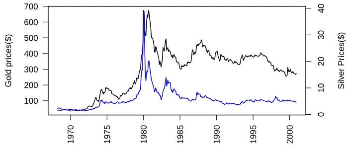
The models were fitted with the data displayed in Figure 3.1. This figure shows the monthly average of London Fix gold prices denoted by yt, and the monthly average

of London Fix silver prices, denoted zt from January of 1969 through December of

2000, for a total of n = 384 observations. The data set is taken from The Pert Mint web site [9]. This web site provides all up to date prices for gold and silver in monthly average and daily average forms.

1970 1975 1980 1985 1990 1995 2000 100 200 300 400 500 600 700 Gold pr ices($) Silv er Pr ices($) 0 10 20 30 40

(34)

3.1 Random Coefficient Model

When we set Φ = 0 in (3.3), the state equation takes the following form:

βt=β+at (3.4)

and this implies that if Φ = 0, then the stochastic parameter model in (3.3) becomes a random coefficient model (3.4) with mean β and variance σ2

a. Additionally, if

σa is small relative to β, the state system becomes nearly deterministic, (βt ≈ β),

simplifying to a classical linear model.

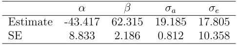
The Newton-Raphson estimation procedures were applied to the gold and silver price data as described in Section 2.2.3. Table 3.1 summarizes the estimates of the fixed parameters vector Θ and the standard errors (SE) associated with each fixed parameter. The results summarized in Table 3.1 indicate that the gold-silver relationship is definitely not deterministic. The time-varying coefficient {βt} in this

model is white noise with constant mean β.

Table 3.1: Fixed Parameters of Random Coefficient Model

α β σa σe

Estimate -43.417 62.315 19.185 17.805 SE 8.833 2.186 0.812 10.358

On the other hand, smoothed βt are not white noise. The Kalman smoothing

procedure allows us to find the estimates of βt for given observations of the silver

and gold prices, {(z1, y1), . . . ,(zn, yn)}, so that we can trace back the smoothed{βt}.

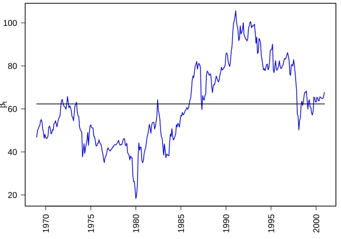
These {βt} actually represent the gold silver price ratio for this model. Figure 3.2

(35)

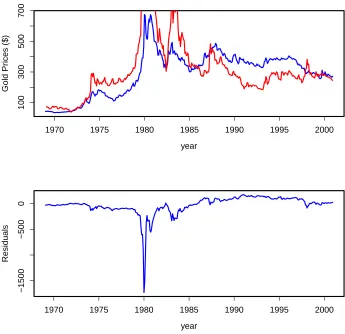
Another result of this model is that the mean of the residual error of prediction is -28.5. We assumed that the prediction error is normally distributed with mean zero. Figure 3.3 shows that the random coefficient model does not support this assumption, therefore, we can conclude that the random coefficient model works poorly and we need to consider another models. It can also be seen from the residuals of this model in Figure 3.3 that the impact of 1980’s silver bubble is very pronounced in this model. The random coefficient model could not handle this unusual occurrence in silver price speculation, which given in Section 2.1.1.

1970 1975 1980 1985 1990 1995 2000

20 40 60 80 100

βt

Figure 3.2: Random coefficient model’s estimates for one step-ahead prediction coefficientsβtis black, estimates for smoothedβtis blue. These parameters represents

(36)

year

Gold Pr

ices ($)

1970 1975 1980 1985 1990 1995 2000

100

300

500

700

year

Residuals

1970 1975 1980 1985 1990 1995 2000

−1500

−500

0

Figure 3.3: Gold prices (blue) random coefficient regression model fit (red) and residuals.

3.2 First-Order Autoregression Coefficient Model

When we don’t set Φ = 0, the state equation (2.5) represents a first-order autore-gressive process, AR(1). The model becomes a stochastic parameter regression model, and the fixed parameter vector for this model is Θ = (Φ, α, β, σ2

a, σe2)

0_{, where} _σ2

a is

variance of at and σe2 is variance of et. The Newton-Raphson estimates of the fixed

(37)

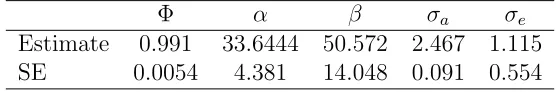
to each fixed parameter, Section 2.2.3. The ML estimate ofφ is very close to 1. This indicates possible violation of causality assumption of AR(1) process. In Figure 3.4, we see that βt is closer to a path of a random walk process than AR(1) [8].

Figure 3.5 shows gold prices (black), model fit (red), and the corresponding residuals. Due to the fact that the model followed the real gold prices very closely and the difference between the price of gold in January of 1696 and December of 2000 was so large, this makes it very difficult to separate gold prices from model fit. This is only a scaling issue. The famous silver bubble of 1980 is clearly shown in residuals. This model could not account for this drastic change in silver prices caused by only a few people; refer to Section 2.1.1.

Figure 3.6 shows that the βt for prediction and for smoothed are very close. If

we use the smoothed estimates of βt as our stochastic regression coefficient, what

we obtain is a representation of historic gold-silver price ratio, while estimates of prediction βt are giving us one step-ahead predictions. There is one interesting

feature here about the gold silver ratio. Contrary to some earlier suggestions that the gold silver ratio should be between 16 and 20, we can see that before 1990 this ratio was much higher than that and has an upward trend. After 1990, the ratio started decreasing and has a downward trend. Both βt for prediction and smoothing

closely follow the gold silver ratio. Further discussion on this subject will be given in Section 3.5 along with economic implications.

Table 3.2: Fixed parameters of first-order autoregression Coefficient model

Φ α β σa σe

(38)

1970 1975 1980 1985 1990 1995 2000 0

20 40 60 80

βt

0.0 0.5 1.0 1.5 2.0 2.5

A

CF

−0.2 0.2 0.6 1.0

0.0 0.5 1.0 1.5 2.0 2.5

P

A

CF

−0.2 0.2 0.6 1.0

(39)

year

Gold Pr

ices

1970 1975 1980 1985 1990 1995 2000

100

300

500

700

year

Residuals

1970 1975 1980 1985 1990 1995 2000

−100

0

50

150

(40)

1970 1975 1980 1985 1990 1995 2000 0

20 40 60 80

βt

Figure 3.6: First-order autoregression Coefficient model’s estimates for one step-ahead prediction coefficientβtis black, estimates for smoothedβt is blue. These parameters

(41)

3.3 random walk with Drift Model

The previous model showed us that the time varying parameters of the stochastic regression model was actually closer to the random walk process than the AR(1) process. This is the reason we investigated the random walk with drift model.

In state equation (3.3), if we set Φ = 1 and keep a constant d on the right side of the equation as a drift constant, the first-order autoregression coefficient model becomes a random walk with drift model,

βt =βt−1+d+at (3.5)

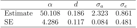
The fixed parameter vector for this model is Θ = (α, d, σa, σe)0. These parameters

are estimated by the Newton-Raphson algorithm procedure and these estimates are listed in Table 3.3. The standard error corresponding to each fixed parameter is also included in the table. In the previous model, we had (1−Φ)β term in (3.2) and its value is 0.45 even though β is 50.575. This is due to Φ ≈ 1; see Table 3.2. In this model, instead of (1−Φ)β, we have drift constant d, which is 0.186. In the limiting case when Φ→1, (1−Φ)β can be considered as a drift constant. Therefore, we can say that previous model had larger drift influence on the model.

Table 3.3: Fixed Parameters of random walk with Drift Model

α d σa σe

Estimate 50.108 0.186 2.323 0.861 SE 4.286 0.117 0.084 0.481

(42)

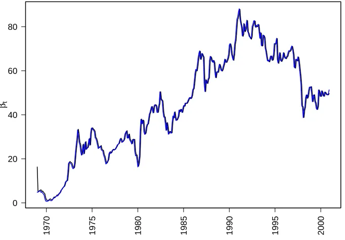
in Figure 3.7 and closely follow each other. Figure 3.8 shows the estimates of one

1970 1975 1980 1985 1990 1995 2000

0 20 40 60 80

βt

Figure 3.7: Random walk with drift model’s estimates for one step-ahead prediction coefficients βt is black and smoothed βt is blue.

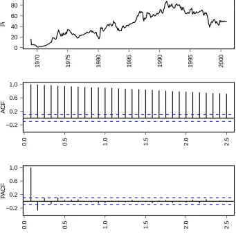
step-ahead predictions, βt, along with its ACF and PACF. This clearly shows that

βt’s path is a typical random walk with drift model. When we compare this with

Figure 3.4, it can be seen that the stochastic parameterβt is more like a random walk

than an AR(1) process.

(43)

1970 1975 1980 1985 1990 1995 2000 0

20 40 60 80

βt

0.0 0.5 1.0 1.5 2.0 2.5

A

CF

−0.2 0.2 0.6 1.0

0.0 0.5 1.0 1.5 2.0 2.5

P

A

CF

−0.2 0.2 0.6 1.0

(44)

year

Gold Pr

ices

1970 1975 1980 1985 1990 1995 2000

100

300

500

700

year

Residuals

1970 1975 1980 1985 1990 1995 2000

−100

0

50

150

(45)

3.4 random walk without Drift Model

When we set φ = 1, in (3.3), this model becomes a random walk without drift,

βt=βt−1+at. When the stochastic regression model’s fixed coefficient estimates for

Φ is nearly 1, this models turns into a random walk model, limΦ→1(Φ−1) ≈ 0. .

It is no surprise that Figure (3.10) of the first-Order autoregression coefficient model and Figure (3.6) of the random walk model are almost identical. The fixed parameter vector for this model is Θ = (α, σa, σe)0. These parameters are estimated by the

Newton-Raphson algorithm procedure and are are listed in Table 3.4. The standard error corresponding each fixed parameter is also included in the table. The difference between these parameters and those of the random walk with drift model are not significant. It appears that the major difference is the drift constant. The standard

Table 3.4: Fixed Parameters of random walk Model

α σa σe

Estimate 46.526 2.262 0.874 SE 3.968 0.077 0.503

error corresponding each fixed parameter is also included in the table. The difference between these parameters and those of the random walk with drift model are not significant. It appears that the major difference is the drift constant. Figure 3.11 shows the estimates of one step-ahead predictions,βt, along with its ACF and PACF.

This clearly shows that βt’s path is a typical random walk model. When we compare

this with Figure 3.4, it can be seen that the stochastic parameter βt is more like a

(46)

1970 1975 1980 1985 1990 1995 2000 0

20 40 60 80

βt

(47)

1970 1975 1980 1985 1990 1995 2000 0

20 40 60 80

βt

0.0 0.5 1.0 1.5 2.0 2.5

A

CF

−0.2 0.2 0.6 1.0

0.0 0.5 1.0 1.5 2.0 2.5

P

A

CF

−0.2 0.2 0.6 1.0

(48)

year

Gold Pr

ices

1970 1975 1980 1985 1990 1995 2000

100

300

500

700

year

Residuals

1970 1975 1980 1985 1990 1995 2000

−100

0

50

150

(49)

3.5 Prediction

Figure 3.13 compares one-step ahead gold price predictions from the four models (random coefficient, first-order autoregression, random walk with drift, and random walk without drift) described in Sections 3.1-3.4, along with gold and silver prices between January of 1969 and December of 2000. Excluding the random coefficient model, all three models closely trace the gold prices. Figure 3.14 displays all four models’ one-step ahead prediction for βt. After the first five years, all three models’

(except the random coefficient model) βt are close to each other.

We compared all four models’ forecastability, as described in Section 2.2.4. Fig-ure 3.15 shows all four models’ prediction of 12 months into the futFig-ure. We see that all four models under predicted gold prices for 2001; the random walk with drift gave the best predictions, and the random coefficient model produced the worst predictions.

While silver closely followed gold trends most of the years between 1969 and 2000, after 2001 this is not true. It appears that silver lost some of its appeal for a short period of time, although there were yet known reasons for this. However, in the political side, a new administration took over the presidential office around 2001. During this time of the political change, gold prices started to rise; silver, on the other hand, was not so quick to respond to this change. We do not know what caused the discrepancy between the gold price forecasts and actual gold prices. However, because the forecasts were close to actual gold prices up to 2000, we conjecture that the predicted values of the gold prices obtained from the random walk with drift model would have been closer to gold prices, if such a change in the political environment was not made.

(50)

0 500 1000 1500 2000

1 ₃₂ ₆₁ ₉₂

122 153 183 214 245 275 306 336 367

Months

Gold Prices ($)

0 10 20 30 40 50

Silver Prices ($)

Gold ARR RW RWD RC Silver

Figure 3.13: Gold, silver prices and model fit of gold for four models: AR(1) coefficient model (ARR), random walk with drift (RWD), random walk (RD), and random coefficient (RC)

(51)

Beta_t for Prediction

-20 0 20 40 60 80 100

1 51 101 151 201 251 301 351

Months

Beta

ARC RC RW RWD

Figure 3.14: βt of one step ahead predictions of four models between January of 1969

and December of 2000

Table 3.5: (SSPE) and (SAPE) of four models’ 2001, 12 months predictions

RC ARC RWD RW

SSE 23327 6524 3094 6183

(52)

200 220 240 260 280 300

1 2 3 4 5 6 7 8 9 10 11 12

Months of 2001

Gold prices ($)

4 4.2 4.4 4.6 4.8 5

Silver Prices($)

gold RC FS RWD RW silver

(53)

CHAPTER 4 CONCLUSIONS

In Section 2.1.1, we listed each historical decisions or events between 1969 and 2000 that caused similar effects in gold and silver prices. During these effects, if there was a spike in the gold prices, there was a spike in the silver prices as well. Based on this historical data, we assumed gold and silver prices were dictated by the same fundamentals (i.e., what affected gold affected silver as well). This lead us to examine the dynamic relationship between gold and silver prices between 1969 and 2000.

The relationship between gold and silver was assumed to follow a stochastic pa-rameter regression model and stochastic papa-rameters were assumed to be a first-order autoregression process, AR(1). We formulated this relationship into a state-space form, and we used the Kalman filter and smoother algorithms to estimate both the fixed parameters and the stochastic regression coefficients. We determined that the stochastic parameters were closer to a random walk process than the AR(1) process. Therefore, we applied random walk process with a drift, random walk without a drift, and random coefficient models. When it comes to forecastability of the four models, the random walk with drift model seems to be the best model even though all four models under estimated gold prices with given silver prices.

(54)

its gold reserve and the U.S. sold around 16 million troy ounces of gold [12]. These last two events caused a bubble-like increase in gold price. Even though the reasons for the increase in gold and silver prices were not related, it appeared that gold and silver followed the same trend.

(55)

REFERENCES

[1] Akgiray, V., Booth, G.G., Hutem, J.J., and Mustafa, C., 1991. “Conditional dependence in precious medal price”.The financial Review, vol. 26, pp. 367–386. [2] Chan, M.L., and Mountain, D.C. 1988. ”The interactive and causal relationship involving precious metal price movement.” Journal of Business and Economic Statistics, vol.6, pp.69–77.

[3] Durbin, J., and Koopman, S.J., Time Series Analysis by State Space Methods.

Oxford University Press, Oxford, 2001.

[4] Escribano, A., and Granger, C. W. J., 1998., ”Investigating the relationship between gold and silver price.” Journal of Forcasting vol.17, pp. 81–107.

[5] Fay, S.,Beyond Greed. The Viking, New York, 1982.

[6] Newbold, P. and Bos, T., 1985,T. Stochastic Parameter Regression Models, Sage, Beverly Hills, 1985

[7] Lee, W., and Lin, H., 2010, ”The dynamic relationship between gold and silver futures markets based on Copula-AR-GJR-GARCH model.” Middle Eastern Finance and Econometrics vol. 7, pp. 118–129.

[8] Shumway, R. H. and Stoffer, D. S., Time Series Analysis and It’s Application with R examples, 3rd edition. Springer, New York, 2011.

[9] The Pert Mint. Monthly Data (all).

http://www.perthmint.com.au/investment invest in gold precious metal prices.aspx

[10] Silver Institute. 2012,Silver In History.

http://www.silverinstitute.org/site/ silver-essentials/silver-in-history/

[11] Silver Institute., 2012, Silver in Technology .

http://www.silverinstitute.org/site/silver-in-technology/

[12] Geology.com. 2012.Gold History.

(56)

[13] Geology.com. 2012.The Many Uses of Gold.

(57)

(58)

APPENDIX A

R-PROGRAMS

This program calculates the fixed parameters of the state space model and the time varying coefficients of the stochastic regression model. It is a modification of the example 6.13 from Shumway and Stoffer [8], and uses tsa3.rda which can be downloaded from the web site provided in [8]. This program can be adapted to other three models by only changing the initial parameters and fixed parameter vector.

# Stochastic Regression Model with

# AR(1) Stochastic parameter Model

# Kfilter2 and Ksmoother2 given Shumway and Stoffer

load("tsa3.rda")

GoldSilverTBill<-read.csv(

file="GoldSilverLondonfix.csv",

head=TRUE,sep=",")

n<-nrow(GoldSilverTBill)

m<-ncol(GoldSilverTBill)

acf2=function(series,max.lag=NULL){

(59)

if (is.null(max.lag)) max.lag=ceiling(10+sqrt(num))

if (max.lag > (num-1)) stop("Number of lags

exceeds number of observations")

ACF=acf(series, max.lag, plot=FALSE)$acf[-1]

PACF=pacf(series, max.lag, plot=FALSE)$acf

LAG=1:max.lag/frequency(series)

minA=min(ACF)

minP=min(PACF)

U=2/sqrt(num)

L=-U

minu=min(minA,minP,L)-.01

ACF<-round(ACF,2); PACF<-round(PACF,2)

return(cbind(LAG, ACF, PACF) )

}

gold<-ts(as.numeric(data.matrix(GoldSilverTBill$GoldLondonFixAMAverage)),

start=c(1968,4),end=c(2012,1),frequency=12) # Gold prices Bid Average

silver<-ts(as.numeric(data.matrix(GoldSilverTBill$SilverLondonFixAverage)),

start=c(1968,4),end=c(2012,1),frequency=12) # Silver Prices Bid Average

#TBill<-ts(as.numeric(data.matrix(GoldSilverTBill$TBilRatio_3month)),

start=c(1968,4),end=c(2012,1),frequency=12)

# Here we change the window max-min values

#cbind(gold,silver)

#dev.new()

(60)

#dev.new()

#plot(cbind(as.numeric(lgold),as.numeric(lsilver)))

yearMin=1969

yearMax=2000

monthMin=1

monthMax=12

y<-window(gold,c(yearMin,monthMin),c(yearMax,monthMax))

z<-window(silver,c(yearMin,monthMin),c(yearMax,monthMax))

# summary(lm(lgold~lsilver))

mu0=16; Sigma0=0.004; phi=0.991860026; alpha=33.644412

b=50.57212; cQ=2.46836910; cR=1.123121

init.par<-c(phi,alpha,b,cQ,cR) # initial parameters

num<-length(y)

A<-array(z,dim=c(1,1,num))

input<-matrix(1,num,1)

# Function to calculate likelihood

Linn<-function(para) {

phi<-para[1]

alpha<-para[2]

b<-para[3]

Ups<-(1-phi)*b

cQ<-para[4]

cR<-para[5]

#kf<-Kfilter2(num,y,A,mu0,Sigma0,phi,Ups,alpha,theta,cQ,cR,0,input)

(61)

return(kf$like)

}

tol<-0.0001

est<-optim(init.par,Linn,NULL,method="BFGS",hessian=TRUE,

control=list(trace=1,REPORT=1,reltol=tol))

SE<-sqrt(diag(solve(est$hessian)))

phi<-est$par[1]

alpha<-est$par[2]

b<-est$par[3]

Ups<-(1-phi)*b

cQ<-est$par[4]

cR<-est$par[5]

u<-rbind(estimate=est$par,SE)

colnames(u)<-c("phi","alpha","b","sig_w","sig_v")

u

#ks=Ksmooth2(num,y,A,mu0,Sigma0,phi,Ups,alpha,tetha,cQ,cR,0,input)

ks=Ksmooth2(num,y,A,mu0,Sigma0,phi,Ups,alpha,1,cQ,cR,0,input)

SE_bsmooth<-(ks$Ps)

SE_bprediction<-(ks$Pp)

SE_bfilter<-(ks$Pf)

################################################################

#log(gold)~log(silver) Model

################################################################

Bsmooth <-ts(as.vector(ks$xs),start=c(yearMin,monthMin),

(62)

Bprediction<-ts(as.vector(ks$xp),start=c(yearMin,monthMin),

end=c(yearMax,monthMax), frequency=12)

Bfilter<-ts(as.vector(ks$xf),start=c(yearMin,monthMin),

sil <-ts(as.vector(z), start=c(yearMin,monthMin),

gol<-ts(as.vector(y), start=c(yearMin,monthMin),

SE_bs<-ts(as.vector(SE_bsmooth),start=c(yearMin,monthMin),

SE_bp<-ts(as.vector(SE_bprediction),start=c(yearMin,monthMin),

SE_bf<-ts(as.vector(SE_bfilter),start=c(yearMin,monthMin),

Bp<-window(Bprediction,c(yearMin,monthMin),c(yearMax,monthMax))

Bs<-window(Bsmooth,c(yearMin,monthMin),c(yearMax,monthMax))

Bf<-window(Bfilter,c(yearMin,monthMin),c(yearMax,monthMax))

postscript(file="FullStochasticBeta.eps",

paper="special",

width=10,

height=7,

horizontal=FALSE)

par(mfrow=c(1,1), mex=0.8)

par(mar=c(4,4,2,2),mfrow=c(1,1), mex=0.8,cex=1.4,lwd=2)

(63)

mtext(bquote(beta[t]),line=2,side=2, cex=1.5)

lines(Bs, col="blue",lwd=2)

#lines(Bf, col="red",lwd=2)

dev.off()

gol_hat <- sil*Bp+alpha

res_gold<- gol-gol_hat

postscript(file="FullStochCoefModel.eps",

paper="special",

width=10,

height=10,

horizontal=FALSE)

par(mfrow=c(2,1), mex=0.8,cex=1.4,lwd=3)

plot(gol, xlab="year", ylab="Gold Prices",col="blue",cex=1.4,lwd=3)

lines(gol_hat, col="red",lwd=3)

plot(res_gold, xlab="year", ylab="Residuals",col="blue",cex=1.4,lwd=3)

dev.off()

x11()

par(mfrow=c(2,1), mex=0.8,cex=1.4,lwd=3)

plot(gol, xlab="year", ylab="Gold Prices",col="blue",cex=1.4,lwd=3)

lines(gol_hat, col="red",lwd=3)

plot(res_gold, xlab="year", ylab="Residuals",col="blue",cex=1.4,lwd=3)

postscript(file="FSacfBp.eps",

paper="special",

width=10,

(64)

horizontal=FALSE)

ACFPCAF<-acf2(Bp)

xx<-dim(ACFPCAF)

LAG<-ACFPCAF[,1]

ACF<-ACFPCAF[,2]

PACF<-ACFPCAF[,3]

minA=min(ACF)

minP=min(PACF)

U=2/sqrt(num)

L=-U

minu=min(minA, minP, L)-0.1

par(mfrow=c(3,1), mex=0.8,cex=1.4, lwd=3)

par(mar = c(4,6,2,0.8)) #, oma = c(1,1.2,1,1), mgp = c(1.5,0.6,0))

plot.ts(Bp,ann=FALSE,las=2)

mtext(bquote(beta[p]), side=2, line=3,cex=1.5)

plot(LAG, ACF, type="h",ylim=c(minu,1),ann=FALSE,las=2,yaxt="n")

mtext("ACF", side=2, line=3,cex=1.5)

axis(side=2, at=c(-0.2, 0.2, 0.6, 1),las=2)

abline(h=c(0,L,U), lty=c(1,2,2), col=c(1,4,4),yaxt="n")

plot(LAG, PACF, type="h",ylim=c(minu,1),ann=FALSE,las=2,yaxt="n")

mtext("PACF", side=2, line=3,cex=1.5)

axis(side=2, at=c(-0.2, 0.2, 0.6, 1),las=2)

abline(h=c(0,L,U), lty=c(1,2,2), col=c(1,4,4))

(65)

postscript(file="FSacfBs.eps",

paper="special",

width=10,

height=10,

horizontal=FALSE)

ACFPCAF<-acf2(Bs)

xx<-dim(ACFPCAF)

LAG<-ACFPCAF[,1]

ACF<-ACFPCAF[,2]

PACF<-ACFPCAF[,3]

minA=min(ACF)

minP=min(PACF)

U=2/sqrt(num)

L=-U

plot.ts(Bs,ann=FALSE,las=2)

mtext(bquote(beta[s]), side=2, line=3,cex=1.5)

plot(LAG, ACF, type="h",ylim=c(minu,1),ann=FALSE,las=2,yaxt="n")

axis(side=2, at=c(-0.2, 0.2, 0.6, 1),las=2)

(66)

axis(side=2, at=c(-0.2, 0.2, 0.6, 1),las=2)

dev.off()

postscript(file="FSacfBf.eps",

paper="special",

width=10,

height=10,

horizontal=FALSE)

ACFPCAF<-acf2(Bf)

xx<-dim(ACFPCAF)

LAG<-ACFPCAF[,1]

ACF<-ACFPCAF[,2]

PACF<-ACFPCAF[,3]

minA=min(ACF)

minP=min(PACF)

U=2/sqrt(num)

L=-U

plot.ts(Bf,ann=FALSE,las=2)

mtext(bquote(beta[f]), side=2, line=3,cex=1.5)

(67)

axis(side=2, at=c(-0.2, 0.2, 0.6, 1),las=2)

plot(LAG, PACF, type="h",ylim=c(minu,1),ann=FALSE,las=2,yaxt="n")

axis(side=2, at=c(-0.2, 0.2, 0.6, 1),las=2)

dev.off()

# This part for data file

sil <-ts(as.vector(z), start=c(yearMin,monthMin),

gol<-ts(as.vector(y), start=c(yearMin,monthMin),

SE_bs<-ts(as.vector(SE_bsmooth),start=c(yearMin,monthMin),

SE_bp<-ts(as.vector(SE_bprediction),start=c(yearMin,monthMin),

SE_bf<-ts(as.vector(SE_bfilter),start=c(yearMin,monthMin),

Bp<-window(Bprediction,c(yearMin,monthMin),c(yearMax,monthMax))

Bs<-window(Bsmooth,c(yearMin,monthMin),c(yearMax,monthMax))

Bf<-window(Bfilter,c(yearMin,monthMin),c(yearMax,monthMax))

NEW_Data<-cbind(sil, gol, gol_hat, res_gold, Bsmooth,

SE_bs,Bprediction,SE_bp,Bfilter, SE_bf);

(68)

# Silver and Gold between 2001-January and 2001-December

y2001<-window(gold,c(2001,1),c(2001,12))

z2001<-window(silver,c(2001,1),c(2001,12))

y2001<-as.vector(as.numeric(y2001))

z2001<-as.vector(as.numeric(z2001))

betaT<-rep(0,12)

y_hat<-rep(0,12)

xp=length(Bp)

xs=length(Bs)

xf=length(Bf)

xpsf<-cbind(Bp, Bs,Bf)

beta<-as.vector(as.numeric(Bp))

# phi, alpha, b, cQ, cR Fixed parameters

betaT0=beta[xp]

betaT[1]=b+phi*(betaT0-b) #+rnorm(1,0, cQ)

y_hat[1]=alpha+betaT[1]*z2001[1] #+rnorm(1,0, cR)

for (i in 2:12){

betaT[i]=b+phi*(betaT[i-1]-b) #+rnorm(1,0, cQ)

y_hat[i]=alpha+betaT[i]*z2001[i] #+rnorm(1,0, cR)

}

SSE=sum( (y_hat-y2001)^2)

SE=sum(abs(y_hat-y2001))

y2001<-ts(as.numeric(y2001),start=c(2001,1),end=c(2001,12),frequency=12)

y_hat<-ts(as.numeric(y_hat),start=c(2001,1),end=c(2001,12),frequency=12)

(69)

write.csv(FS_prediction, file="Prediction_FS.csv",na="NA")

postscript(file="FSPrediction.eps",

paper="special",

width=10,

height=7,

horizontal=FALSE)

par(mar = c(5,6,2,0.8), mfrow=c(1,1), mex=0.8,cex=1.2,lwd=3)

plot(y2001,xlab="Year 2001", ylim=c(min(y2001, y_hat),

max(y2001, y_hat)),ylab="Gold Prices ($)",

col="blue",lwd=3)

lines(y_hat,col="red",lwd=3)

dev.off()

gol_1<-append(gol, y2001,after=length(gol))

gol_hat_1<-append(gol_hat, y_hat, after=length(gol_hat))

gol_1<-ts(gol_1,start=c(1969,2),end=c(2001,12),frequency=12)

gol_hat_1<-ts(gol_hat_1,start=c(1969,2),end=c(2001,12),frequency=12)

res_gold_1<- gol_1-gol_hat_1

colnames(u)<-c("phi","alpha","b","sig_w","sig_v")

u

SSE