Image Motion Direction Detection Based on L-K Optical Flow Method

(1)

Vol. 7, 2017, 95-106

ISSN: 2349-0632 (P), 2349-0640 (online) Published 17 June 2017

www.researchmathsci.org

DOI: http://dx.doi.org/10.22457/jmi.v7a12

95

Journal of

Image Motion Direction Detection Based on

L-K Optical Flow Method

Chao Jiang

College of Science, Chongqing University of Posts and Telecommunications Chongqing – 400065, Chongqing, China. E-mail: evan_j0416 @163.com

Received 19 May 2017; accepted 14 Jun 2017

Abstract. It is difficult to determine the direction of the motion of the image with less time to analyze the series of images taken in the camera movement at a lower resolution. In this paper, a method of L-K optical flow and S-T corner detection is proposed to study the motion direction of the field of view in the image sequence. On this basis, the weighted least squares method is used to further reduce the error. At the same time, the model is extended from two-dimensional to three-dimensional space, so that the model is more universal.

Keywords: Sparse L-K optical flow method; weighted least squares method; S-T corner detection; image motion direction detection

1. Introduction

The key problem is to judge the moving direction by analyzing a series of image captured in the slow-moving camera with less time at a lower resolution. Paper gray scale processing [1], L-K optical flow method [2], ST corner detection methods [3] were used in this paper to study the image sequence vision area in direction of motion.

First of all, shoot a picture at each certain time interval, using Photoshop software to down these pictures’ resolution to 32*64, to simulate the low-resolution image in shooting equipment. Because only considering into the monochrome images, then turn those pictures into grayscale pattern, thus the average brightness was replaced by the grayscale value. The value of each pixel in the image is grayscale values for each lattice.

Second, given camera in slow movement this feature, we establish a method model based on gradient of L-K light flow, on all adjacent of two frame pictures for calculation obtained light flow field, light flow field instead of playground, judge figure in the all objects of overall movement direction, take its anti-direction that for vision regional of movement direction, on all light flow field for overlay judge out vision regional overall of movement direction [4]. In order to increase the precision, weighted least squares was introduced [5], using the weighting function of the original weighted operation.

(2)

96

Finally, putting forward a model based on 3D motion and structure estimation of continuous optical flow, and I generalize the model from 2D to 3D. But it will greatly increase the calculation time to analyze the 3D moving of objects detailedly. So this paper only contain the method to realize the model but does not contain case analysis and further discussion。.

2. Grayscale processing

For the sake of simplicity, only the monochrome imaging is assumed and the resolution of the imaging is assumed to be 32 x 64. The color multi-frame picture pixels taken from the video are adjusted to 32 x 64 by using programming software or image processing software and converted to gray Degree image.

Using Photoshop software and MATLAB software can be directly processed to achieve the image of the gray-scale conversion shown in Figure 1. The goal of converting to a grayscale image is to replace the luminance mean with its gray scale value in monochrome imaging, making further calculations quicker and faster.

Figure 1: the n-1th picture the nth picture .

3. Establishment of optical flow model 3.1.Optical flow method

An optical flow is a movement pattern that refers to the apparent movement of an object, surface, and edge formed by an observer (such as an eye, a camera, etc.) and a background in a perspective. Optical flow technology, such as motion detection and image segmentation, time collision, motion compensation coding, three-dimensional parallax, are the use of this edge or surface movement of the technology. The optical flow is the instantaneous velocity of the pixel motion of the space moving object on the observed imaging plane. The study of the optical flow is to use the time domain variation and correlation of the pixel intensity in the image sequence to determine the motion of the respective pixel position, the relationship between the change of time and the structure of the object and its movement in the scene.

(3)

97

Figure 2: the relationship between the movement field and the optical flow field The movement field is the movement of the object in the three-dimensional real world; the optical flow field is the projection of the playground on the two-dimensional image plane. The instantaneous two-dimensional velocity field contains important information about the depth, curvature and orientation of the visible surface of the object, and the relative motion between the object and the sensor system in the scene.

The premise of the optical flow is assumed to be:

(1) Constant brightness: The brightness between adjacent frames is constant;

(2) Small movement: The frame time of the next video frame is continuous, that is, the motion of objects between adjacent frames is "tiny";

(3) Spatial consistency: To maintain spatial consistency; That is, the same sub-image pixels have the same movement;

Assuming that the gray value of the point on the image at time t is( , , , )x y z t , the gray value I x y z t( , , , ) , at time t+ ∆t , this movement is reached

(x+

δ

x y, +

δ

y z, +

δ

z)，and the corresponding gray value is

( , , )

I x+

δ

x y+

δ

y z+

δ

z , which is assumed to be equal toI x y z t( , , , )：

, , , ) ( , , , )

I x y z t = I x+

δ

x y+

δ

y z+

δ

z t+

δ

t

（

Figure 3: pixel displacement diagram

(4)

98

( , , , )

( , , , ) . . .

I x x y y z z t t

I I I I

I x y z t x y z t H O T

x y z t

δ

+ + + + =

∂ ∂ ∂ ∂

+ + + + +

∂ ∂ ∂ ∂

Since the move is small enough to ignore the second and higher order (H.O.T) terms, we can get from this equation:

0

I I I I

x y z t

x

δ

y

δ

z

δ

t

δ

∂ ₊∂ ₊∂ ₊∂ ₌

∂ ∂ ∂ ∂ or 0

I x I y I z I t x t y t z t t t

δ

∂ ₊∂ ₊∂ ₊∂ ₌

∂ ∂ ∂ ∂

This is recorded as:

( , , , ) dx u x y z t

dt

=

( , , , ) dy v x y z t

dt

=

(But cannot accurately determine the component of the optical flow in the vertical direction of the gradient, the following will be negated on the z), so that the gradient of a certain direction, with a first-order difference instead of the light flow in the horizontal direction, First order differential, to get the optical flow constraint equation:

0

x y t

I u+I v+ =I

where x , y , t

I I I

x y t

∂ ∂ ∂

= = =

∂ ∂ ∂ , write the gradient form as IT U It 0

→

∇ ⋅ + = . Since the optical flow field ( , )T

U = u v has two variables, and only one of the basic constraint equations can only find the value of the optical flow field along the gradient direction, it is an ill-posed problem to solve the optical flow field from the basic optical flow equation. Constraints, which is the so-called optical flow algorithm aperture problem. Then to find the optical flow vector will need another set of solutions.

Write the above formula as a matrix multiplication in the form:

[

x y t

u

I I I

v  

_{ }_{= −}

   3.2.L-K optical flow method

(5)

99 coordinates.

Assuming that the pixel stream is consistent in a small window of size m * m (m> 1), then the following set of equations can be obtained from pixels 1 ... n, n = m ^ 2:

1 1 1

2 2 2

...

x x y y t

xn x yn y tn I U I U I I U I U I

I U I U I

+ = −   + = −     ₊ _{= −} 

It can be seen that the pixel is 32 * 64. This system is clearly an overdetermined equation, that is to say there is redundancy in the system. The equations can be further expressed as:

1 1 ₁

2 2 2

x y _t

x y x t

y

tn xn yn

I I _I

I I U I

U I I I   _₋ _   _ _ −     ₌_ _     _ _     _ _ −       M M M

Referred to as:_Aur= −_b

Using the least squares method to solve this overdetermined equation, there are:

( )

T T

A Av=A −b or

1

( T ) T( )

v A A A b

→

−

= −

we can get :

2

x xi xi yi xi yi

y xi yi yi yi ti

U I I I I I

U I I I I I

  ₋    =      ₋       

∑

where the summation is from 1 to n.

This means that looking for optical flow can be summed up by the reciprocal of the images on three dimensions, but we also need a weight function

( , , ), , , [1, ]

W i j k i j k∈ m to highlight the coordinates of the center of the window.

The lack of this algorithm is that it cannot produce a very high density flow vector, for example, in the movement of the edge and the black large homogeneous region of the small mobile information flow will soon fade, it has the advantage of the presence of noise Stick is still good.

Using the MATLAB software, we get the velocity vector of the pixels between two images, which can be roughly moved in the direction of the arrow, that is, the camera moves in the opposite direction.

(6)

100 3.3.Weighted least squares method

In the L-K algorithm based on the use of weighted least squares method to further reduce the error [8], the specific steps are as follows: consider a point ( , )x y ，Build around it

*

N =n n of the field Λ，And assuming an optical flow ( , )T

U = u v In the field Λ remain unchanged. For each pixel value in the domain Λwe can establish a constraint equation for it, then there are 2

n optical flow constraint equations in the domain, where the Kth pixel constraint equation is:：

0

xk yk tk

I

⋅ +

u

I v

+

I

=

Our goal is to minimize

2 ( , )

( ( , ) _t)

x y

I x y U I

∈Λ ∇ ⋅ +

∑

_{by least squares method.}

The light flow constraint for each pixel in the neighborhood is the same for the objective function. In order to improve the accuracy of the optical flow estimation and reduce the error, we use the weighted least squares method to estimate the two components of the optical flow. The weighting equation for the pixel point of the neighborhood is given a higher weight, and the neighborhood of the neighborhood has a smaller weight, that is, minimizing the target:

2 ( , )

( , )( ( , ) t)

x y

W x y I x y U I

∈Λ

∇ ⋅ +

∑

where W is the window function, has a higher value at the center of the neighborhood, and the edge point has a smaller value. Expressed in matrices：

T T

A WA U⋅ = A W b⋅

among them,，W =diag W x y[ ( ,₁ ₁),W x y( ,₂ ₂),...,W x( _N,y_n)]，

1 1

[ ( , ),..., ( _N, _N)]T

A= ∇I x y ∇I x y ，b= −[ ( ,I x yt ₁ ₁),..., (I xt N,yN)]。

2 ( , ) ( , )

( , ) ( , )

x x y

x y x y

T

x y y

x y x y

W x y I W x y I I A WA

W x y I I W x y I

∈Λ ∈Λ ∈Λ ∈Λ

 

 

= 

 

 

∑

，

It is a 2 * 2 matrix, when it is reversible, can be closed solution:

1

( T ) T

U = A WA − A Wb。

In this way, the confidence of the optical flow can be estimated. Assuming the eigenvalue of _{A WA}T _is

1 2

λ λ

≥ , when

λ τ

2 > （

τ

is the threshold set）,use 1

( T ) T

U = A WA − A Wb to estimate light flow is reliable. Based on the above statement, it is necessary to extract the pixels with large eigenvalues in the image, and then use the LK algorithm to calculate the optical flow of these pixels, which will greatly reduce the judgment time. The image processed by the weighted least squares method can more clearly judge the direction of the trajectory.

(7)

101

Through the above analysis, you can take a sparse optical flow algorithm, do not need to calculate the optical flow of each pixel, the algorithm can save time. It contains two processes. First, the pixels with larger eigenvalues in the extracted image are the same. The principle is the same as the corner detection method. Therefore, the process can use the corner detection algorithm Shi-Tomasi to detect the corner points. Second, the optical flow is calculated using the L-K method at the extracted corners。

4.1.Shi-Tomasi corner detection

Shi-Tomasi corner detection algorithm is an improvement of Harris corner detection[9] algorithm. Corner point is a local feature point, at the corner, the gray scale of the first derivative is the local maximum, the gray scale of the image in all directions have changed [9]. Let the image get gray I x y( , )at point( , )x y . Create a n n* window Λ centered on that point, move the window[∆ ∆x, y], the resulting gray scale is changed

( , )

E ∆ ∆x y as the following formula:

2 ( , )

( , ) ( , )[ ( , ) ( , )]

x y

E x y W x y I x x y y I x y

∈Λ

∆ ∆ =

∑

+ ∆ + ∆ −

For tiny translations, to carry out I x( + ∆x y, + ∆y) Taylor expansion and ignore second and above items, brought into the formula above is

2 2 2 2

( , ) ( , ) ( , )

( , ) ( , ) _x 2 ( , ) _x _y ( , ) _y

x y x y x y

E x y x W x y I x y W x y I I y W x y I

∈Λ ∈Λ ∈Λ

∆ ∆ = ∆

∑

+ ∆ ∆

∑

+ ∆

∑

_,

where Ix and Iy represent the partial derivative of the image grayscale in the direction x and the direction y, and write the above formula as a matrix:

( , ) [ , ] x

E x y x y M y

∆

 

∆ ∆ = ∆ ∆ _∆ 

 

M is an 2 * 2 matrix,

2 ( , ) ( , )

( , ) ( , )

x x y

x y x y

x y y

x y x y

W x y I W x y I I M

W x y I I W x y I

∈Λ ∈Λ ∈Λ ∈Λ

 

 

= 

 

 

∑

Whether the pixel ( , )x y is the corner is through the matrix M to judge. At first, the Harris algorithm subtracts the determinant of the matrixM 's determinant and the difference from the pre-given threshold to obtain the corner point. In this paper, Shi-Tomasi algorithm is used to select the appropriate window size and window function, calculate the matrix M corresponding to each pixel and its eigenvalues, and then set the corresponding threshold to extract the corners in the image.

4.2.Calculate the optical flow at the corner

(8)

102

detection and L-K optical flow calculation to select the same window size and window function, so T

M = A WA ，This is not necessary to calculate the optical flow T

M = A WA, The use of corner detection process to calculate the matrix M to calculate the optical flow, which will greatly save the algorithm running time. Therefore, when calculating the optical flow at the corner, the selected window size and window function are consistent with the corner detection algorithm. And since the two eigenvalues at the corners are greater than 0, the matrix M is reversible，so 1 T

U =M A Wb− 。 5. Model promotion

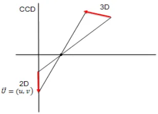
Since the model established in this paper is simplified as the motion direction detection of the two-dimensional plane, the method of extending it to three-dimensional motion is given, but it is not well studied.

In the optical flow method to increase the parameter z that the vertical direction of the vector component, when the camera moves to the left and right at the same time while moving to the left or right at the same time, there will be three-dimensional movement of the situation. If you want to determine how an object or a camera is moving in three dimensions, you're going to introduce a three-dimensional motion and structure estimation model based on continuous light flow.

Three-dimensional motion estimation refers to estimating the three-dimensional motion parameters of the object from the two-dimensional image sequence and the three-dimensional mechanism [10]. Specifically, assume that the object has a point M relative to the camera coordinates from time

_t

_k to time

_t

_k₊₁ , the position from

( _k, , _k) k

y

x

z

to ₁ ₁

1

( _k , , _k )

k

y

x

+ +

z

+ . Its projection on the two-dimensional image plane

is

1 1

' '

( , )

k

y

k

x

+ ₊ . And then by analyzing the two-dimensional motion to restore the

three-dimensional movement of objects and objects on the depth of interest points. There are many algorithms for three-dimensional structure estimation, such as three-dimensional structure from stereo vision, dimensional structure from motion recovery, three-dimensional structure from light and dark, and so on.

The three-dimensional motion estimation optical flow method is based on the estimation of the optical flow field. The motion and structure of the three-dimensional object are estimated from the images of two steamed dumplings or the projection. The optical flow method requires a dense optical flow field, Match the obvious feature points.

The relative motion of the rigid body relative to the observer is represented in the three-dimensional space coordinate system, whose origin is at the vertex of the perspective projection, and the Z-axis direction follows the center of the field of view. In this coordinate system, the instantaneous motion of the rigid body is expressed by the average velocityV =(VX + +VY VZ) and the rotation speed Ω = Ω + Ω + Ω( X Y Z)to represent. The two-dimensional sequence image is obtained from the object perspective to the plane perpendicular to the Z axis, and the origin of the image coordinate system ( , )x y In the position of the three-dimensional space( , , )X Y Z =(0, 0,1), That is, the image is located at the unit focal length (set f =1in the motion analysis of the practice).

(9)

103 (position determined by vector_R→) is:

( )

X V R

→ → →

= − + Ω×

In the Cartesian coordinate system, the rigid body three-dimensional motion can be expressed as a three-dimensional rotation and three-dimensional translation and that:

_X→ ₌₍_{R X T}→₊→₎ (1) where: R is a 3 × 3 rotation matrix (can be expressed in different forms, such as Cartesian coordinates of the Euler angle, anti-symmetric matrix, quaternion, etc.);

[

1, 2, 3

]

t T T T T

→

= is a three-dimensional translation vector;

[

, ,

]

t

X X Y Z

→

= and '

[

' ' '

, , t

X X Y Z

→



= _ Respectively represent the coordinates of an entity point at the moment t and '

trelative to the center of the rotor.

Equation (1) provides an expression for two instantaneous three-dimensional displacements, since the two instantaneous intervals ∆t are close to zero, with

The infinitesimal Euler angles represent the rotation matrix, and for the (1) type to the limit, an expression of the three-dimensional instantaneous velocity can be obtained,

0 0

0

Y X

Z

Z X Y

X

Y Z

V

X X

Y Y V

Z Z V

Ω

−Ω   



   

  



 _{= Ω} _−Ω  ₊

  



   

  



  _−Ω _Ω  

      

(2)

At each moment, the point P is projected onto the coordinates of the image plane p（）（x y, = X Z Y Z/ , / ）, and

' '

' _X _{X Z}

u x

Z Z Z

= = −

' ' ' _Y _{Y Z}

v y

Z Z Z

= = −

By (2) finishing

2

[ (1 ) ] [ ]

[(1 ) ] [ ]

Z X

X Y Z

Z Y

X Y Z

V V

u xy x y x

Z Z V V

v y xy x y

Z Z

= Ω − + Ω + Ω + −

= + Ω − Ω − Ω + −

(3)

The equations (3) are the Longuet-Higgins and prazdny optical flow equations10. From the relationship between the translation velocity (V V V_X, _Y, _Z)and the fractional relationship of Z, we can see that the absolute scale of the depth Z is uncertain and if Z = 0, then Z cannot be determined. So translational motion is a necessary condition for discovering the structure.

(10)

104

the image center coordinate system. Assuming that the surface is continuous and differentiable, the Taylor series of the central local surface around the optical axis is expanded:

2 2

0 3

1 1

( , )

2 2

X Y XX XY YY

Z=Z +Z X +Z Y+ Z X +Z XY+ Z Y +O X Y (4)

0 0

Z > ,Z0 is the distance from the optical axis to the origin，ZX,ZY is the slope relative to the X, Y axis,ZXX,ZYY,ZXYare the curvatures, the last term is the high-order item that can be fused. Equation (4) is represented by image coordinates.

2 2 1

0 3

1 1

( , ) [1 ( , )]

2 2

X Y xx xy yy

Z x y =Z −Z x+Z y+ Z x +Z xy+ Z y +O x y − (5) Substituting (5) into (3)

2 2

3 0 0

2

1 1

( , ) [ ][1 ( , )]

2 2

[ (1 ) ]

Z X

X Y xx xy yy

X Y Z

V V

u x y x Z x Z y Z x Z xy Z y O x y Z Z

xy x y

= − − − − − − − +

Ω − + Ω + Ω

(6)

2 2

3 0 0

2

1 1

( , ) [ ][1 ( , )]

2 2

[(1 ) ]

Z Y

X Y xx xy yy

X Y Z

V V

v x y y Z x Z y Z x Z xy Z y O x y Z Z

y xy x

= − − − − − − − +

+ Ω − Ω − Ω

(7)

Considering the optical flow field analytic structure as well as the surface assumption is smooth (such as continuous and differentiable), the image point velocity in the image origin of a small neighborhood can be developed into Taylor series:

2 2

0 3

1 1

( , ) ( , )

2 2

x y xy xy xy

u x y = +u u x u y+ + u x +u xy+ u y +o x y (8)

2 2

0 3

1 1

( , ) ( , )

2 2

x y xy xy xy

v x y = +v v x v y+ + v x +v xy+ v y +o x y (9)

among them: u u v v u_x, _y, _x, _y, _xx,u_xy,u_yy,v_xx,v_xy,v_yy are the optical flow field partial derivative,O x y3( , ) is the higher order items that can be ignored，considering (6),(7)

(11)

105

0 0

2 2

x Y

y X

x z x X

v z y Y

y Z Z Y

x Z y X

xx x X x xx Y

xy z Y x xy X

yy x yy

xx y xx

xy z X y xy Y

yy z Y y yy X

u V

v V

u V V Z v V V Z

u V Z

v V Z

u V Z V Z u V Z V Z u V Z

v V Z

v V Z V Z v V Z V Z

= − − Ω = − + Ω

= + = + = Ω + = −Ω +

= − + − Ω

= − + + Ω

= =

= − + − Ω

= − + + Ω

(10)

This formula was originally proposed by Longuet-Higgins and Prazdny [1980], which also leads to a higher partial derivative of the optical flow, but in general it takes the second order. There are only 11 unknowns in the 12 equations of equation (10). These 12 equations are collectively referred to as the elephant equation. Of the 12 nonlinear equations of the image flow equation, 11 unknowns consist of 5 structural parameters(Slope Z_X,Z_Y and the relative curvature Z_xx,Z_xy,Z_yy ） and 6 motion parameters（Rotate parameters Ω Ω Ω_X, _Y, _Zand 3 ratio translation speed V V V_x, _y, _z）。

Although the equations are in general terms, in general, solutions are unique, but because of the non-linearity of equations, in some cases, multiple solutions will inevitably arise.

The sequence of motion analysis based on optical flow is: (1) Calculate the optical flow first

(12)

106 REFERENCES

[1] Frank R. Giorano, William P.Fox, Steven B. Horton. Mathematical Modeling (Original Edition 5), Beijing: Mechanical Industry Press, 2015.

[2] Zhang Yicheng, Study on Moving Object Recognition Algorithm in Low Resolution Traffic Video, Beijing: University of Science and Technology, 2014

[3] Zhu Jun, Ren Mingwu, Zhang Yang Jing, Zhao Wei, Fast matching algorithm based on corner detection, Nanjing University, 6 (2011) 755-758.

[4] Jiang Zhijun, Yi Huarong, A feature tracking method based on image pyramid optical flow, Journal of Wuhan University, 8 (2007) 680-683.

[5] B.Lucas and T.Kanade, An iterative image registration technique with an application to stereo vision, Proc. of 7th International Joint Conference on Artificial Intelligence (IJCAI), pp. 674-679, 1981.

[6] Pan Shi-zhu, Shu Wei-qun, Wang Xing, Intelligent detection of real-time moving objects based on adaptation background, Journal of Computer Applications, 10 (2004) :95-96.

[7] Wu Jiaojiao, Based on the global movement of video segmentation and motion recognition algorithm, China Ocean University, 2013.

[8] Mei Jiangyuan, Si Yulin, Gao Huijun, Detection and recognition of moving object across the camera, Automation Technology & Applications, 11 (2011) 43-46.

[9] Wang Wei, Tang Yiping, Renjuan Li, Bing Chuan, Li Peilin, Han Huating, An improved Harris corner extraction algorithm, Precision Optical Engineering, 10 (2008)1995-2001.