https://doi.org/10.5194/gmd-11-4195-2018 © Author(s) 2018. This work is distributed under the Creative Commons Attribution 4.0 License.
(GO)
2
-SIM: a GCM-oriented ground-observation
forward-simulator framework for objective evaluation
of cloud and precipitation phase
Katia Lamer1, Ann M. Fridlind2, Andrew S. Ackerman2, Pavlos Kollias3,4,5, Eugene E. Clothiaux1, and Maxwell Kelley2
1Department of Meteorology and Atmospheric Science, Pennsylvania State University, University Park, PA 16802, USA 2NASA Goddard Institute for Space Studies, New York, New York 10025, USA
3Environmental & Climate Sciences Department, Brookhaven National Laboratory, Upton, New York 11973, USA 4School of Marine and Atmospheric Sciences, Stony Brook University, Stony Brook, New York 11794, USA 5University of Cologne, 50937 Cologne, Germany
Correspondence:Katia Lamer ([email protected]) Received: 7 April 2018 – Discussion started: 30 May 2018
Revised: 14 September 2018 – Accepted: 17 September 2018 – Published: 16 October 2018
Abstract. General circulation model (GCM) evaluation us-ing ground-based observations is complicated by inconsis-tencies in hydrometeor and phase definitions. Here we de-scribe (GO)2-SIM, a forward simulator designed for ob-jective hydrometeor-phase evaluation, and assess its perfor-mance over the North Slope of Alaska using a 1-year GCM simulation. For uncertainty assessment, 18 empirical rela-tionships are used to convert model grid-average hydrome-teor (liquid and ice, cloud, and precipitation) water contents to zenith polarimetric micropulse lidar and Ka-band Doppler radar measurements, producing an ensemble of 576 forward-simulation realizations. Sensor limitations are represented in forward space to objectively remove from consideration model grid cells with undetectable hydrometeor mixing ra-tios, some of which may correspond to numerical noise.
Phase classification in forward space is complicated by the inability of sensors to measure ice and liquid signals dis-tinctly. However, signatures exist in lidar–radar space such that thresholds on observables can be objectively estimated and related to hydrometeor phase. The proposed phase-classification technique leads to misphase-classification in fewer than 8 % of hydrometeor-containing grid cells. Such mis-classifications arise because, while the radar is capable of detecting mixed-phase conditions, it can mistake water- for ice-dominated layers. However, applying the same classifi-cation algorithm to forward-simulated and observed fields
should generate hydrometeor-phase statistics with similar uncertainty. Alternatively, choosing to disregard how sensors define hydrometeor phase leads to frequency of occurrence discrepancies of up to 40 %. So, while hydrometeor-phase maps determined in forward space are very different from model “reality” they capture the information sensors can pro-vide and thereby enable objective model evaluation.
1 Introduction
Active remote sensing observations remain an indirect ap-proach to evaluate models because they measure hydrome-teor properties different from those produced by microphys-ical schemes. For each hydrometeor species within a grid cell models prognose geophysical quantities such as mass and number concentration, whereas active remote sensors measure power backscattered from all hydrometeor species present within their observation volumes. Defining which hy-drometeors have an impact is a fundamental question that needs to be addressed by the modeling, as well as observa-tional, communities. In numerical models it is not uncom-mon to find very small hydrometeor mixing ratio amounts as demonstrated below. They may possibly be unphysical, ef-fectively numerical noise, and the decision of which hydrom-eteor amounts are physically meaningful is somewhat arbi-trary. Considering sensor capabilities is one path to objec-tively assessing hydrometeor populations within models. On such a path it is possible to evaluate those simulated hydrom-eteor populations that lead to signals detectable by sensors, leaving unassessed those not detected. Sensor detection ca-pabilities are both platform and sensor specific. Space-borne lidars can adequately detect liquid clouds globally but their signals cannot penetrate thick liquid layers, limiting their use to a subset of single-layer systems or upper-level cloud decks (Hogan et al., 2004). Space-borne radar observations, while able to penetrate multilayer cloud systems, are of coarser ver-tical resolution and of limited value near the surface owing to ground interference and low sensitivity (e.g., Huang et al., 2012b; Battaglia and Delanoë, 2013; Huang et al., 2012a). A perspective from the surface can therefore be more appropri-ate for the study of low-level cloud systems (e.g., de Boer et al., 2009; Dong and Mace, 2003; Klein et al., 2009; Intrieri et al., 2002).
Fortunately, both sensor sampling and hydrometeor scat-tering properties can be emulated through the use of for-ward simulators. Forfor-ward simulators convert model output to quantities observed by sensors and enable a fairer com-parison between model output and observations; discrepan-cies can then be more readily attributed to dynamical and mi-crophysical differences rather than methodological bias. For example, the CFMIP (Cloud Feedback Model Intercompari-son Project) Observation Simulator Package (COSP) is com-posed of a number of satellite-oriented forward simulators (Bodas-Salcedo et al., 2011), including a lidar-backscattering forward simulator that has been used to evaluate the repre-sentation of upper-level supercooled water layers in GCMs (e.g., Cesana and Chepfer, 2008; Kay et al., 2016). Also, Zhang et al. (2018) present a first attempt at a ground-based radar reflectivity simulator tailored for GCM evaluation.
Here we propose to exploit the complementarity of ground-based vertically pointing polarimetric lidar and Doppler radar measurements, which have been shown uniquely capable of documenting the water phase of shallow and multilayered clouds that form near the surface and fre-quently contain supercooled water layers. More specifically,
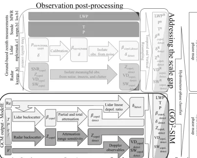
we present a GCM-oriented ground-observation forward-simulator ((GO)2-SIM) framework designed for objective hydrometeor-phase evaluation (Fig. 1). GCM output vari-ables (Sect. 2) are converted to observvari-ables in three steps: (1) hydrometeor-backscattered power estimation (Sect. 3), (2) consideration for sensor capabilities (Sect. 4), and (3) es-timation of specialized observables (Sect. 5). These forward-simulated fields, similar to observed fields, are used as inputs to a multi-sensor water-phase classifier (Sect. 6). The perfor-mance of (GO)2-SIM is evaluated over the North Slope of Alaska using output from a 1-year simulation of the current development version of GCM ModelE. Limitations and un-certainty are discussed in Sects. 6.3 and 7, respectively.
2 GCM outputs required as inputs to the forward simulator
To demonstrate how atmospheric model variables are con-verted to observables we performed a 1-year global simu-lation using the current development version of the ModelE GCM. Outputs from a column over the North Slope of Alaska (column centered at latitude 71.00◦and longitude−156.25◦) are input to (GO)2-SIM. The most relevant changes from a recent version of ModelE (Schmidt et al., 2014) are the im-plementation of the Bretherton and Park (2009) moist turbu-lence scheme and the Gettelman and Morrison (2015) mi-crophysics scheme for stratiform cloud. The implementa-tion of a two-moment microphysics scheme with prognos-tic precipitation species makes this ModelE version more suitable for the forward simulations presented here than pre-vious versions. Here ModelE is configured with a 2.0◦ by
2.5◦latitude–longitude grid with 62 vertical layers. The
ver-tical grid varies with height from 10 hPa layer thickness over the bottom 100 hPa of the atmosphere, coarsening to about 50 hPa thickness in the mid-troposphere, and refining again to about 10 hPa thickness near the tropopause. For the current study, the model top is at 0.1 hPa, though we limit our analy-sis to pressures greater than 150 hPa. Dynamics (large-scale advection) are computed on a 225 s time step and column physics on a 30 min time step. High-time-resolution outputs (every column physics time step) are used as input to (GO)2 -SIM. ModelE relies on two separate schemes to prognose the occurrence of stratiform and convective clouds. The current study focuses on stratiform clouds because their properties are more thoroughly diagnosed in this model version; when performing future model evaluation, the contribution from convective clouds will also be considered.
T P q f V GC M ou tp ut -Mode lE Lidar backscatter Radar backscatter
Partial and total attenuation Attenuation range sensitivity Doppler observables !copol "copol Re !copol detect SNRcopol Zcopol VDcopol SWcopol Ra da r ka zr ge .b 1 Lida r mp lc ma sk .c 1 Ground -ba se d ze nith m ea sure m ents #$%&$'%((, $%'' * H yd ro m ete or -p ha se c la ss ifi er LWP. PR TR ! copol, detect .
δdetect.
Z copol, detect . VD copol, detect . SW copol, detect . H yd ro m et eo r-ph as e ma p T P LWP Zcopol, detect VDcopol, detect SWcopol, detect !$%&$'%(( * !copol,detect *detect So nd e wnpn. b1 MW R los. b1 Da ta q ua lit y c on tro l Calibration Isolate
obs. from noise
LWP T P !copol, detect *detect Zcopol, detect VDcopol, detect SWcopol, detect H yd ro m et eo r-ph as e ma p VDcopol detect SWcopol detect δdetect Zcopol detect Te m po ra l a nd V er tic al Res ampl ing Lidar linear depol. ratio
Observation post-processing
Ad
dr
es
sin
g t
he
sc
ale
g
ap
(G
O
)
2-SIM
Sect. 2. Sect. 3. Sect. 4. Sect. 5.
Isolate meaningful obs. from noise, insects, and clutter
Sect. 6.
Figure 1.(GO)2-SIM framework. (GO)2-SIM emulates two types of remote sensors: Ka-band Doppler radars (dark gray shading) and 532 nm polarimetric lidars (light gray shading). It then tunes and applies a common phase-classification algorithm (white boxes) to both observed (upper section) and forward-simulated (bottom section) fields. Follow-on work will describe how observation can be post-processed and resampled to reduce the scale gap before model evaluation can be performed.
37.8 % pure ice, and 59.8 % mixed in phase (Table 1a). How-ever, these statistics are impacted by a number of simulated small hydrometeor mixing ratio amounts that may or may not result from numerical noise (e.g., Fig. 2a; blueish green colors). The forward-simulator framework will be used to create phase statistics of only those hydrometeors present in amounts that can create a signal detectable by sensors, hence removing the need for arbitrary filtering.
(GO)2-SIM forward-simulator inputs are, at model native resolution, mean grid box temperature and pressure as well as hydrometeor mixing ratios, area fractions (used to esti-mate in-cloud mixing ratios), mass-weighted fall speeds, and effective radii for four hydrometeor species: cloud liquid wa-ter, cloud ice, precipitating liquid wawa-ter, and precipitating ice. In its current setup, (GO)2-SIM can accommodate any model that produces these output variables
3 Hydrometeor-backscattered power simulator
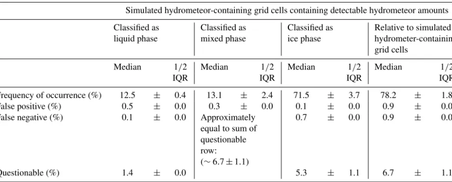
Table 1. (a)Hydrometeor-phase frequency of occurrence obtained(a)from ModelE mixing ratios outside of the forward-simulator frame-work and(b–c)from the forward-simulation ensemble created using different backscattered power assumptions. The median and interquartile range (IQR) capture the statistical behavior of the ensemble. Results using thresholds(b)objectively determined for each forward-ensemble member and(c)modified from those in Shupe (2007). Percentage values are relative either to the total number of simulated hydrometeor-containing grid cells (426 603) or those grid cells with detectable hydrometeor amounts (333 927). Note that the total number of simulated grid cells analyzed is 981 120.
(a)Determined using ModelE output hydrometeor mixing ratios
Simulated hydrometeor-containing grid cells Containing
only liquid phase
Containing mixed phase
Containing only ice phase
Relative to total number of simulated grid cells
Frequency of occurrence (%) 2.4 59.8 37.8 43.5
(b)Determined using flexible objective thresholds estimated using model output mixing ratios
Simulated hydrometeor-containing grid cells containing detectable hydrometeor amounts Classified as
liquid phase
Classified as mixed phase
Classified as ice phase
Relative to simulated hydrometer-containing grid cells
Median 1/2 Median 1/2 Median 1/2 Median 1/2
IQR IQR IQR IQR
Frequency of occurrence (%) 11.3 ± 0.6 19.2 ± 1.8 68.8 ± 3.1 78.3 ± 1.8
False positive (%) 0.5 ± 0.0 1.1 ± 0.3 0.0 ± 0.0 1.7 ± 0.3
False negative (%) 0.2 ± 0.0 Approximately
equal to sum of questionable row: (∼5.2±0.9)
1.5 ± 0.2 1.7 ± 0.3
Questionable (%) 1.4 ± 0.0 3.8 ± 0.9 5.2 ± 0.9
Total error (%) 6.9 ± 1.1
(c)Determined using fixed empirical thresholds modified from Shupe (2007)
Simulated hydrometeor-containing grid cells containing detectable hydrometeor amounts Classified as
liquid phase
Classified as mixed phase
Classified as ice phase
Relative to simulated hydrometer-containing grid cells
Median 1/2 Median 1/2 Median 1/2 Median 1/2
IQR IQR IQR IQR
Frequency of occurrence (%) 12.5 ± 0.4 13.1 ± 2.4 71.5 ± 3.7 78.2 ± 1.8
False positive (%) 0.5 ± 0.0 0.3 ± 0.0 0.1 ± 0.0 0.9 ± 0.0
False negative (%) 0.1 ± 0.0 Approximately
equal to sum of questionable row: (∼6.7±1.1)
0.7 ± 0.0 0.9 ± 0.0
Questionable (%) 1.4 ± 0.0 5.3 ± 1.1 6.7 ± 1.1
Hydrometeor mixing ratios (kg kg-1) Hydrometeor fall velocity (m s-1) Hydrometeor effective radius (mm) C lo ud liq . C lo ud ic e P re cip . li q.. P re cip . ic e Date (mm/dd/yy) a1)
a2)
a3)
a4)
b1)
b2)
b3)
b4)
c1)
c2)
c3)
c4)
-40℃
0℃
08/08/12 08/12/12 08/16/12 08/08/12 08/12/12 08/16/12 08/08/12 08/12/12 08/16/12
Date (mm/dd/yy) Date (mm/dd/yy)
Hei gh t ( km ) Hei gh t ( km )Hei gh t ( km ) Hei gh t ( km
) 10 0.0 0.5 1.0 1.5 2.0 0.001 0.01 0.1 1
-15 10-10 10-5
0 4 8 12 0 4 8 12 0 4 8 12 0 4 8
12 ) ) )
) ) )
) ) )
) ) )
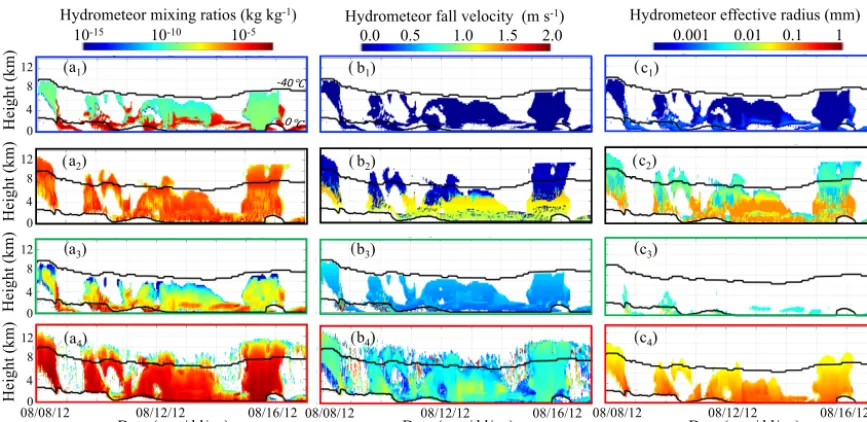
Figure 2.Sample time series of ModelE outputs:(a1–4)mixing ratios,(b1–4)mass-weighted fall speed (positive values indicate downward
motion) and(c1–4)effective radii for cloud droplets (1; blue boxes), cloud ice particles (2; black boxes), precipitating liquid drops (3; green boxes), and precipitating ice particles (4; red boxes). Also indicated are the locations of the 0 and−40◦C isotherms (horizontal black lines).
output hydrometeor effective radius. Their approach, based on Mie theory, relies on the assumption that cloud particles (both liquid and ice) are spherical and requires additional as-sumptions about hydrometeor size distributions and scatter-ing efficiencies. Similarly, the COSP (Bodas-Salcedo et al., 2011) and ARM Cloud Radar Simulator for GCMs (Zhang et al., 2018) packages both use QuickBeam for the estimation of radar-backscattered power (i.e., radar reflectivity; Haynes et al., 2007). QuickBeam computes radar reflectivity using Mie theory, again under the assumption that all hydrometeor species are spherical and by making additional assumptions about the shape of hydrometeor size distributions as well as mass–size and diameter–density relationships. While some of these assumptions may be consistent with the assump-tions in model cloud microphysical parameterizaassump-tions, some are not adequately realistic (e.g., spherical ice) or complete for accurate backscattering estimation and it is typically very difficult to establish the sensitivity of results to all such as-sumptions.
To avoid having to make ad hoc assumptions about hy-drometeor shapes, orientations, and compositions, which are properties that also remain poorly documented in na-ture, (GO)2-SIM employs empirical relationships to convert model output to observables. These empirical relationships are based on observations, direct or retrieved, with their own sets of underlying assumptions and are expected to capture at least part of the natural variability in hydrometeor proper-ties. Additionally, empirical relationships are computation-ally less expensive to implement than direct radiative scatter-ing calculations, thus enablscatter-ing the estimation of an ensem-ble of backscattering calculations using a range of
assump-tions in an effort to quantify part of the backscattering uncer-tainty (see Sect. 7). The empirical relationships proposed re-quire few model inputs, potentially enhancing consistency in applying (GO)2-SIM to models with differing microphysics scheme assumptions and complexity. Section 6 will show that, while the empirical relationships employed in (GO)2 -SIM may not be as exact as direct radiative scattering cal-culations, they produce backscattering estimates of sufficient accuracy for hydrometeor-phase classification, which is the main purpose of (GO)2-SIM at this time.
3.1 Lidar-backscattered power simulator
At a lidar wavelength of 532 nm, backscattered power is pro-portional to total particle cross section per unit volume. Ow-ing to their high number concentrations, despite their small size, cloud particles backscatter radiation of this wavelength the most.
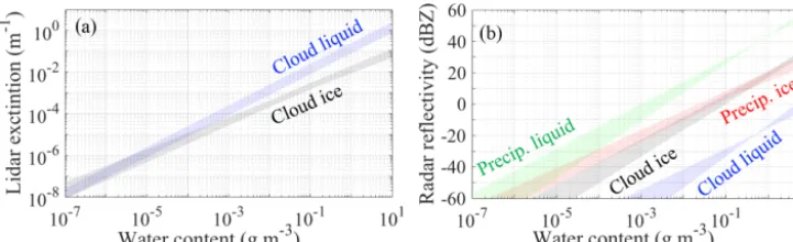
atmo-Figure 3.Relationship between water content in the form of cloud liquid (blue), precipitating liquid (green), cloud ice (black) and precipitat-ing ice (red) and(a)lidar extinction, and(b)radar copolar reflectivity. Spread emerges from using multiple differing empirical relationships (listed in Table 2) and from variability in the 1-year ModelE output (including the effects of varying temperature and effective radii).
spheric temperature and hydrometeor effective radius vari-ability). Figure 3a also illustrates the fundamental idea that lidar extinction increases with increasing water content and that for a given water content cloud droplets generally lead to higher lidar extinction than cloud ice particles.
Lidar copolar-backscattered power (βcopol,species; m−1sr−1) generated by each hydrometeor species is related to lidar extinction (σcopol,species; m−1) through the lidar ratio (Sspecies; sr):
βcopol,cl=(1
Scl) σcopol,cl, (6)
βcopol,ci=(1Sci) σcopol,ci. (7) While constant values are used for the lidar ratios of liq-uid and ice clouds in this version of the forward simulator, we acknowledge that in reality they depend on particle size. O’Connor et al. (2004) suggest that a liquid cloud lidar ratio (Scl) of 18.6 sr is valid for cloud liquid droplets smaller than 25 µm, which encompasses the median diameter expected in the stratiform clouds simulated here. Kuehn et al. (2016) ob-served layer-averaged lidar ratios in ice clouds (Sci) ranging from 15.1 to 36.3 sr. Sensitivity tests indicate that adjusting the ice cloud lidar ratio to either of these extreme values in the forward simulator increases the number of detectable hy-drometeors by no more than 0.6 %, changes the hydrometeor-phase frequency of occurrence statistics by less than 0.4 %, and causes less than a 0.1 % change in water-phase classifi-cation errors (not shown). Given these results, the ice cloud lidar ratio is set to the constant value of 25.7 sr, which corre-sponds to the mean value observed by Kuehn et al. (2016).
It is important to consider the fact that lidars do not mea-sure cloud droplet backscattering independently of cloud ice particle backscattering. Rather, they measure total copolar-backscattered power (βcopol,total), which is the sum of the contribution from both cloud phases.
3.2 Radar-backscattered power simulator
At the cloud-radar wavelength of 8.56 mm (Ka band), backscattered power is approximately related to the sixth
power of the particle diameter and inversely proportional to the forth power of the wavelength. Hereafter radar-backscattered power will be referred to as “radar reflectivity” as commonly done in the literature.
(GO)2-SIM relies on water-content-based empirical rela-tionships to estimate cloud liquid water (cl), cloud ice (ci), precipitating liquid water (pl), and precipitating ice (pi) radar reflectivity. Different relationships are used for each species to account for the fact that hydrometeor mass and size both affect radar reflectivity. A number of empirical relationships link hydrometeor water content to copolar radar reflectiv-ity; 13 of these empirical relationships are implemented in (GO)2-SIM (Table 2, Eqs. 8–20, and references therein) and used to generate an ensemble of forward simulations. Fig-ure 3b illustrates the fact that for all these empirical relation-ships increasing water content leads to increasing radar re-flectivity. As already mentioned, radar reflectivity is approx-imately related to the sixth power of the particle size, which explains why, for the same water content, precipitating hy-drometeors are associated with greater reflectivity than cloud hydrometeors.
In reality, radars cannot isolate energy backscattered by individual hydrometeor species. Rather, they measure total copolar reflectivity (Zcopol,total; mm6m−3), which is the sum of the contributions from all of the hydrometeor species.
4 Sensor capability simulator
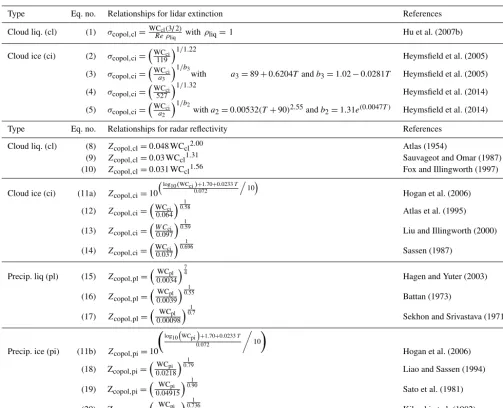
Table 2.Empirical relationships used to convert hydrometeor in-cloud hydrometeor water content (WC; g m−3) to lidar extinction (σ; m−1) and radar reflectivity (Z; mm6m−3).
Type Eq. no. Relationships for lidar extinction References
Cloud liq. (cl) (1) σcopol,cl=WCRe ρcl(3liq/2)withρliq=1 Hu et al. (2007b)
Cloud ice (ci) (2) σcopol,ci=
WCci
119
1/1.22
Heymsfield et al. (2005)
(3) σcopol,ci=
WCci
a3
1/b3
with a3=89+0.6204Tandb3=1.02−0.0281T Heymsfield et al. (2005)
(4) σcopol,ci=
WC
ci 527
1/1.32
Heymsfield et al. (2014)
(5) σcopol,ci=
WC
ci
a2
1/b2
witha2=0.00532(T+90)2.55andb2=1.31e(0.0047T ) Heymsfield et al. (2014)
Type Eq. no. Relationships for radar reflectivity References
Cloud liq. (cl) (8) Zcopol,cl=0.048 WCcl2.00 Atlas (1954)
(9) Zcopol,cl=0.03 WCcl1.31 Sauvageot and Omar (1987)
(10) Zcopol,cl=0.031 WCcl1.56 Fox and Illingworth (1997)
Cloud ice (ci) (11a) Zcopol,ci=10
log10(WCci)+1.70+0.0233T
0.072
.
10
Hogan et al. (2006)
(12) Zcopol,ci=
WCci
0.064
0.158
Atlas et al. (1995)
(13) Zcopol,ci=
W C
ci 0.097
0.159
Liu and Illingworth (2000)
(14) Zcopol,ci=
WCci
0.037
0.6961
Sassen (1987)
Precip. liq (pl) (15) Zcopol,pl=
WC
pl 0.0034
74
Hagen and Yuter (2003)
(16) Zcopol,pl=
WC
pl 0.0039
0.155
Battan (1973)
(17) Zcopol,pl=
WC
pl
0.00098
01.7
Sekhon and Srivastava (1971)
Precip. ice (pi) (11b) Zcopol,pi=10
log10WCpi+1.70+0.0233T
0.072
,
10
!
Hogan et al. (2006)
(18) Zcopol,pi=
WC
pi 0.0218
0.179
Liao and Sassen (1994)
(19) Zcopol,pi=
WC
pi
0.04915
0.190
Sato et al. (1981)
(20) Zcopol,pi=
WC
pi
0.05751
0.7361
Kikuchi et al. (1982)
4.1 Lidar detection capability
Following the work of Chepfer et al. (2008), the (GO)2-SIM lidar forward simulator takes into consideration the fact that lidar power is attenuated by clouds. Attenuation is related to cloud optical depth (τ), which is a function of total cloud extinction (σcopol,total; m−1) that includes the effect of cloud liquid water and cloud ice via
τ (h)=Xh
i=0σcopol,total(i)1i, (21)
Lidar attenuation is exponential and two-way as it affects the lidar power on its way out and back:
βcopol,total,att=βcopol,totale−2ητ. (22) Note that in some instances multiple scattering occurs be-fore the lidar signal returns to the sensor, thus amplifying the
returned signal. In theory, the multiple scattering coefficient (η) varies from 0 to 1. Sensors with large fields of view, such as satellite-based lidars, are more likely to be impacted by multiple scattering than others (Winker, 2003). In the cur-rent study, for which a ground-based lidar is simulated, a multiple scattering coefficient of unity is used. A sensitiv-ity test in which this coefficient was varied from 0.7, such as that implemented in the CALIPSO satellite lidar simula-tor of Chepfer et al. (2008), to 0.3, representing an extreme case, indicated that multiple scattering had a negligible im-pact (less than 1 %) on the number of hydrometeors detected, the hydrometeor-phase frequency of occurrence statistics, and hydrometeor-phase classification error (not shown).
2013) such that total copolar-backscattered power detected (βcopol,total,detect) is
βcopol,total,detect=βcopol,total,att whereτ ≤3;
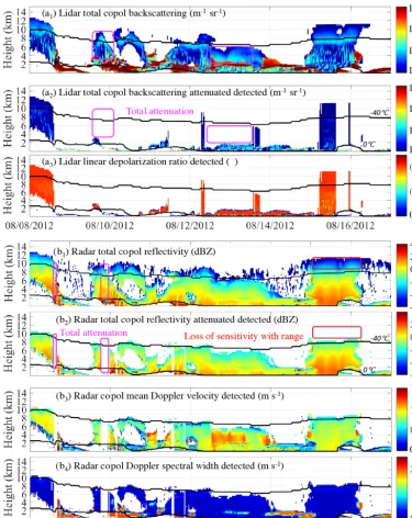
βcopol,total,detect=undetected whereτ >3. (23) For the sample ModelE output shown in Fig. 2, Fig. 4a illustrates results from the lidar forward simulator for one forward-ensemble member (i.e., using a single set of lidar-backscattered power empirical relationships, specifi-cally Eqs. 1 and 4). Figure 4a1 shows lidar total copolar-backscattered power without consideration of sensor limita-tions, such as attenuation, which are included in Fig. 4a2. Lidar attenuation prevents the tops of deep systems contain-ing supercooled water layers from becontain-ing observed (e.g., ma-genta boxes on 10 and 13 August). For the 1-year sample the forward-simulated lidar system detects only 35.5 % of sim-ulated hydrometeor-containing grid cells. In Sect. 6 we will determine which hydrometeors (liquid water or ice) are re-sponsible for the detected signals.
4.2 Radar detection capability
Millimeter-wavelength radars are also affected by signal at-tenuation. Radar signal attenuation depends on both the transmitted wavelength and on the mass and phase of the hy-drometeors. Liquid-phase hydrometeors attenuate radar sig-nals at all millimeter radar wavelengths, even leading to total signal loss in heavy rain conditions. In contrast, water vapor attenuation is less important at relatively longer wavelengths (e.g., 8.56 mm; the wavelength simulated here) but can be important near wavelengths of 3.19 mm (the CloudSat oper-ating wavelength; Bodas-Salcedo et al., 2011).
At 8.56 mm (Ka band), total copolar attenuated reflectivity (Zcopol,total,att; dBZ) is given by
Zcopol,total,att(h)= Zcopol,total(h) −2Xh
i=0
a WCpl(i)+WCcl(i)
1i, (24)
where attenuation is controlled by the wavelength-dependent attenuation coefficient a (dB km−1 (g m−3)−1), which we take to be 0.6 at Ka band (Ellis and Vivekanandan, 2011), by the water contents of cloud liquid (WCcl; g m−3) and pre-cipitating liquid (WCcl; g m−3), and by the thickness of the liquid layer.
In addition to attenuation, radars suffer from having a fi-nite sensitivity that decreases with distance. Given this, the total copolar reflectivity detectable (Zcopol,total,detect; dBZ) is
Zcopol,total,detect=Zcopol,total,attwhereZcopol,total,att≥Zmin
Zcopol,total,detect =Undetected whereZcopol,total,att< Zmin, (25a)
where the radar minimum detectable signal (Zmin; dBZ) is a function of height (h; km) and can be expressed as
Zmin(h)=Zsensitivity at 1 km+20log10(h) . (25b) A value ofZsensitivity at 1 km= −41 dBZ is selected to reflect the sensitivity of the Ka-band ARM Zenith Radar (KAZR) currently installed at the Atmospheric Radiation Measure-ment (ARM) North Slope of Alaska observatory. This value has been determined by monitoring 2 years of observations and it reflects the minimum signal observed at a height of 1 km. The minimum detectable signal used in the simulator should reflect the sensitivity of the sensor used to produce the observational benchmark to be compared to the forward-simulator output.
For the sample ModelE output shown in Fig. 2, Fig. 4b illustrates results from the radar forward simulator for one forward-ensemble member (i.e., using a single set of radar reflectivity empirical relationships, specifically Eqs. 9, 11a, b, and 15). Figure 4b1shows radar total copolar reflectivity without consideration of sensor limitations, while Fig. 4b2 includes the effects of attenuation and the range-dependent minimum detectable signal. Sensor limitations make it such that heavy-rain-producing systems cannot be penetrated (e.g., magenta box on 8 and 10 August) and the tops of deep systems cannot be observed (e.g., red box on 15 August). For the 1-year sample the forward-simulated radar system could detect only 69.9 % of the simulated hydrometeor-containing grid cells. In Sect. 6 we will determine the phase of the hy-drometeors responsible for the detected signals.
4.3 Lidar–radar complementarity
Figure 4.Example outputs from the (GO)2-SIM backscattered power modules (1), sensor capability modules (2), and specialized-observables modules (3–4) for(a)lidars and(b)radars obtained using one set of empirical backscattered power relationships. This figure highlights sensor limitations ranging from attenuation (magenta boxes) to sensitivity loss with range (red boxes). Also indicated are the locations of the 0 and
−40◦C isotherms (black lines). Note that positive velocities indicate downward motion.
5 Forward simulation of specialized observables
In the previous section total copolar-backscattered powers are used to determine which simulated hydrometeors are present in sufficient amounts to be detectable by sensors, hence removing numerical noise from consideration. How-ever, determining the phase of the detectable hydrometeor
populations can be achieved with much greater accuracy by using additional observables.
available from lidar depolarization ratios and radar Doppler spectral widths.
5.1 Lidar depolarization ratio simulator
So far we have described how hydrometeors of all types and phases affect copolar radiation. It is important to note that radiation also has a cross-polar component, which is only af-fected by nonspherical particles. Ice particles, which tend to be nonspherical, are expected to affect this component, while we assume that cloud droplets, which tend to be spherical, do not. Taking the ratio of cross-polar to copolar backscattering thus provides information about the dominance of ice parti-cles in a hydrometeor population. This ratio is referred to as the linear depolarization ratio(δdetect)and it can be estimated where hydrometeors are detected by the lidar.
δdetect=
βcrosspol,ci,detect+βcrosspol,cl,detect βcopol,total,detect
(26a)
According to an analysis of CALIPSO observations by Cesana and Chepfer (2013), cloud ice particle cross-polar backscattering (βcrosspol,ci,detect; m−1sr−1) and cloud liquid droplet cross-polar backscattering (βcrosspol,cl,detect; m−1sr−1) can be approximated using the following relation-ships:
βcrosspol,ci,detect=0.29(βcopol,ci,detect+βcrosspol,ci,detect), (26b)
βcrosspol,cl,detect=1.39(βcopol,cl,detect+βcrosspol,cl,detect)2
+1.76 10−2(βcopol,cl,detect+βcrosspol,cl,detect)≈0. (26c) For reasons mentioned in Sect. 4.1, multiple scattering is considered negligible in the current study such that cloud-liquid droplet cross-polar backscattering is assumed to be zero under all conditions.
5.2 Radar Doppler moment simulator
Specialty Doppler radars have the capability to provide in-formation about the movement of hydrometeors in the radar observation volume. This information comes in the form of the radar Doppler spectrum, which describes how backscat-tered power is distributed as a function of hydrometeor veloc-ity (Kollias et al., 2011). The zeroth moment of the Doppler spectral distribution (the spectral integral) is radar reflectiv-ity, the first moment (the spectral mean) is mean Doppler ve-locity (VD), and the second moment (the spectral spread) is Doppler spectral width (SW). Rich information is provided by the velocity spread (i.e., SW) of the hydrometeor pop-ulation, including information regarding the number of co-existing species, turbulence intensity, and spread of the hy-drometeor particle size distributions. Typically, the effects of turbulence and hydrometeor size variations on the velocity spread for a single species are much smaller than the effect of mixed-phase conditions. As such, Doppler spectral width is a useful parameter for hydrometeor-phase identification.
Forward simulations of Doppler quantities have been performed for cloud models using bin microphysics (e.g., Tatarevic and Kollias, 2015) but not, to our knowledge, for GCMs using two-moment microphysics schemes.
Copolar mean Doppler velocity and copolar Doppler spec-tral width are subject to the same detection limitations as radar reflectivity. In fact, just like radar reflectivity, these observables are strongly influenced by large hydromete-ors; that is, they are reflectivity-weighted velocity aver-ages. Our approach begins by quantifying the contribution of each species present (Pspecies), which is determined by the species detected copolar reflectivity (Zcopol,species,detect; mm6m−3) relative to the total detected copolar reflectivity (Zcopol,total,detect; mm6m−3):
Pspecies=
Zcopol,species,detect Zcopol,total,detect
, (27a)
together with
Zcopol,species,detect(h)=Zcopol,species(h) −2Xh
i=0
a WCpl(i)+WCcl(i)1i
whereZcopol,total,att(h)≥ Zmin(h). (27b) In Eqs. (27a)–(27b) the subscript “species” represents cl, ci, pl, or pi. The attenuation coefficient (a), minimum de-tectable signal (Zmin), and water contents (WCs) are as in Eqs. (24) and (25b). Total mean Doppler velocity detected (VDcopol,detect; m s−1) is the reflectivity-weighted sum of the mass-weighted fall velocity of each hydrometeor species (Vspecies; m s−1):
VDcopol,detect=
X
species=cl,pl,ci,pi
PspeciesVspecies, (28)
where the mass-weighted fall velocity of each hydrometeor species (Vspecies; m s−1) is a model output. Total Doppler spectral width (SWcopol,detect; m s−1) is more complex and can be estimated following a statistical method similar to that described by Everitt and Hand (1981). It takes into consider-ation the properties of each individual hydrometeor species through their respective fall speed (Vspecies; m s−1) and spec-tral width (SWspecies; m s−1) in relation to the properties of the hydrometeor population as a whole through the total mean Doppler velocity detected (VDcopol,detect) estimated in Eq. (28):
SWcopol,detect= (29)
s X
species=cl,pl,ci,pi
Pspecies
SWspecies2+ Vspecies−VDcopol,detect2
,
For the sample ModelE output shown in Fig. 2, Fig. 4b3 and b4 respectively show examples of forward-simulated mean Doppler velocity and Doppler spectral width estimate using one set of empirical radar reflectivity relationship.
6 Water-phase classifier algorithm
From a purely numerical modeling perspective the simplest approach to defining the phase of a hydrometeor population contained in grid cells is to consider any nonzero hydrome-teor mixing ratio species as contributing to the phase of the population. Using this approach, in the 1-year sample, we find that the detectable hydrometeor-containing grid cells are 2.4 % pure liquid, 19.4 % pure ice, and 78.2 % mixed phase (note how these water-phase statistics differ by up to 18.4 % from Sect. 2 in which all grid cells potentially including nu-merical noise were considered). But determining hydrome-teor phase in observational space is not as straightforward. It is complicated by the fact that sensors do not record ice- and liquid-hydrometeor returns separately but rather record total backscattering from all hydrometeors. Retrieval algorithms are typically applied to the observed total backscattering to determine the phase of hydrometeor populations. However, phase-classification algorithms have limitations that require each hydrometeor species to be present not only in nonzero amounts but in amounts sufficient to produce a phase signal. Thus, hydrometeor-phase statistics obtained from a numeri-cal model in the absence of a forward simulator are not nec-essarily comparable with equivalent statistics retrieved from observables, especially in instances in which one hydrom-eteor species dominates the grid cell and other species are present in trace amounts. A common hydrometeor-phase def-inition must be established to objectively evaluate the phase of simulated hydrometeor populations using observations, which requires the development of a phase-classification al-gorithm that can be applied to observables both forward sim-ulated and real.
The scientific literature contains a number of phase-classification algorithms with different levels of complexity. Hogan et al. (2003) used regions of high lidar-backscattered power as an indicator for the presence of liquid droplets. Lidar-backscattered power combined with the lidar lin-ear depolarization ratio has been used to avoid some of the misclassifications encountered when using backscattered power alone (e.g., Yoshida et al., 2010; Hu et al., 2007a, 2009, 2010; Sassen, 1991) Hogan and O’Connor (2004) proposed using lidar-backscattered power in combination with radar reflectivity. While the combination of radar- and lidar-backscattered powers is useful for the identification of mixed-phase conditions, their combined extent remains lim-ited to single-layer clouds or to lower cloud decks because of lidar signal attenuation. Shupe (2007) proposed a tech-nique in which radar Doppler velocity information is used as an alternative to lidar backscattering information (for ranges
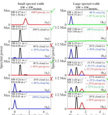
beyond that of lidar total attenuation) to infer the presence of supercooled water in multilayer systems. Figure 5 displays cartoons of Doppler spectra that have the same total copo-lar radar reflectivity but different total mean Doppler veloci-ties (VDs) and Doppler spectral widths (SWs) resulting from different hydrometeor species and combinations, thus high-lighting the added value of Doppler information. The contri-bution of each species to the total copolar reflectivity is indi-cated as a percentage in the top right of each subpanel. These scenarios show that VD tends to be relatively small for pure liquid cloud (Fig. 5a6), pure ice cloud (Fig. 5a2), and even mixed-phase non-precipitating cloud (Fig. 5a3, a5, b3) and only tends to increase when precipitation is present in cloud (Fig. 5a4, b3, b4, b5) or below cloud (Fig. 5a1, b2), making VD a seemingly robust indicator for precipitation occurrence but not for phase identification. These scenarios also show that SW tends to be relatively small in single-phase clouds without precipitation (Fig. 5a2, a6), pure precipitating ice (Fig. 5a1), and multispecies clouds with a dominant hydrom-eteor species (Fig. 5a3, a5). On the other hand, SW tends to be large when liquid precipitation is present (Fig. 5b1, b2, b5) and in mixed-phase clouds without a dominant species (Fig. 5b3, b4, b5). These scenarios suggest that large spectral widths are useful indicators for the presence of supercooled rain and mixed-phase conditions. Scenarios in which this in-terpretation of spectrum width is incorrect will be discussed in Sect. 6.3.
Regardless of which observation they are based on, the aforementioned phase-classification schemes all rely on the assumption that hydrometeor phases when projected on ob-servational space (e.g., lidar-backscattered power against the lidar depolarization ratio) create well-defined patterns that can be separated using thresholds.
6.1 Observational thresholds for hydrometeor-phase identification
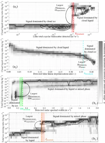
While the thresholds used for the radar reflectivity, lidar-backscattered power, and lidar depolarization ratio are gen-erally accepted by the remote sensing community, the same cannot be said about the radar Doppler velocity and Doppler spectral width thresholds suggested by Shupe (2007). Be-cause simulated mixing ratios of liquid and ice hydrome-teors are known in the (GO)2-SIM framework, the use and choice of all such thresholds for phase classification can be evaluated using joint frequency of occurrence histograms of hydrometeor mixing ratios for a single species and forward-simulated observable values (resulting from all hydrometeor types; Fig. 6). This exercise is repeated for each forward sim-ulation of the ensemble in order to provide a measure of un-certainty and ensure that the choice of empirical relationship does not affect our conclusions.
Figure 5.Cartoon examples of radar Doppler spectra from different hydrometeor combinations: precipitating ice (red), cloud ice (black), precipitating water (green), and cloud water (blue). The contribution of each hydrometeor species to the total copolar reflectivity is indicated in the top right of each subpanel. Each radar Doppler spectrum has been normalized to have the same total copolar radar reflectivity, which highlights the fact that different hydrometeor combinations generate unique mean Doppler velocity (VD) and Doppler spectral width (SW) signatures. As discussed in Sect. 6, low spectral width signatures are assumed to be associated with ice conditions (columna), while high spectral width signatures are assumed to be associated with liquid–mixed-phase conditions (column b). Hydrometeor combinations that respect these assumptions are marked with√marks. Exceptions to these rules (Xmarks) are responsible for (GO)2-SIM phase misclassifi-cations above the level of lidar extinction. This list is not exhaustive.
with the objective of isolating cloud ice particles from cloud water droplets (Fig. 6a1, black contour lines). Two distinct clusters are evident in the joint histogram in Fig. 6a1: (1) βcopol,total,detect between 10−6.7 and 10−5.1m−1sr−1 for cloud liquid water mixing ratios between 10−10.6 and 10−8.8kg kg−1, which we conclude result primarily from cloud ice particle contributions, and (2) βcopol,total,detect between 10−4.6and 10−3.8m−1sr−1for cloud liquid water mixing ratios between 10−6.4 and 10−4.3kg kg−1, which we conclude result primarily from cloud liquid droplet contributions. Therefore, a threshold for best distinguishing these two distinct populations should lie somewhere between 10−5.1and 10−4.6m−1sr−1.
To objectively determine an appropriate threshold to sep-arate different hydrometeor populations, we start by normal-izing the joint histogram of mixing ratio values for fixed ranges of observable values of interest. This normalization is done by assigning a value of 1 to the frequency of occur-rence of the most frequently occurring mixing ratio value per observable range. It is then possible to evaluate the change in this most frequently occurring mixing ratio as a function of observable value. The observable value that intersects the largest change in most frequently occurring mixing ratio is then set as the threshold value.
Figure 6.Example of joint frequency of occurrence histograms (contours) and normalized subsets from the joint histograms (gray shading) for one (GO)2-SIM forward realization:(a1)βcopol,total,detect,(a2)δdetect,(b1)SWcopol,detect, and(b2)Zcopol,total,detect. These are used
for the determination of objective water-phase classifier thresholds (vertical colored dashed lines) that are set at the observational value with the largest change (see curved arrows) in most frequently occurring mixing ratio. These thresholds are not fixed but rather reestimated for each forward-ensemble member. The widths of the color-shaded vertical columns represent the interquartile range spreads generated from 576 different forward realizations.
The dotted black line in Fig. 6a1 connects these most fre-quently occurring mixing ratio values. A curved arrow points to the largest change in most frequently occurring mixing ratio as a function of βcopol,total,detect. A red dashed line at 10−4.9m−1sr−1indicates the lidar backscatter value that
real-Icefinal
βcopol,total,detect[m-1sr-1]
2dete
ct
[
]
Icefinal
Zcopol,total,detect[dBZ]
VD
co
po
l,d
et
ect
[m
s
-1]
< 0.24-0.31 m s-1
<0.30 m s-1 Where SWcopol,detect
> 0.24-0.31 m s-1
> 0.30 m s-1
Liquidfinal
Mixed-phasefinal
Zcopol,total,detect[dBZ]
VD
co
po
l,d
et
ect
[m
s
-1]
Where SWcopol,detect
Liquidfinal
Mixed-phasefinal
Zcopol,total,detect[dBZ]
VD
co
po
l,d
et
ect
[m
s
-1]
Li
q
u
id
in
itia
l
2) Use radar where Liquidinitial and within 750m from cloud top if liquid was detected
1) Use lidar everywhere it detects
Inconclusiveinitial
3) Use radar where lidar does not detect or lidar initial classification is inconclusive
4) Use radar where lidar does not detect or lidar initial classification is inconclusive )
)
)
)
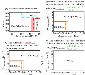
Figure 7.Collective illustration of hydrometeor-phase classification thresholds and phase-classification sequence. Fixed empirical thresholds modified from Shupe (2007) are displayed as gray lines. The objectively determined flexible thresholds are displayed using dashed colored lines and colored shading as in Fig. 6. Note that positive velocities indicate downward motion.
izations of this version of ModelE outputs, the interquartile range of βcopol,total,detect threshold values ranged from 10−5 to 10−4.85m−1sr−1(red shaded vertical column).
The different panels in Fig. 6 show that similar observa-tional patterns occur in the water mixing ratio versus lidar or radar observable histograms such that objective thresh-olds for hydrometeor-phase classification can be determined for all of them. The second threshold determined is for the detected lidar linear depolarization (δdetect), once again with the goal of separating returns dominated by cloud droplets versus cloud ice particles (Fig. 6a2). If we first identify the model grid cells with backscattered power above the lidar detectability threshold of 10−6m−1sr−1, the threshold to distinguish between ice particles and liquid droplets is 0.36 (cyan dashed line). In the 576 forward realizations from this version of ModelE this threshold is stable at 0.36. Note that this threshold is not allowed to fall below 0.05 m s−1.
The third threshold determined is the radar detected copo-lar spectral width (SWcopol,detect) value that separates ice-dominated from liquid- or mixed-phase-ice-dominated returns (Fig. 6b1). We isolate the model grid cells with subzero tem-peratures and look for the most appropriate SWcopol,detect threshold between 0.2 and 0.5 m s−1to isolate the ice
popula-tion. For the example forward simulation we find a threshold of 0.31 m s−1(green dashed line), and over all forward real-izations this threshold ranges from 0.24 to 0.31 m s−1(green shaded vertical column).
The last threshold determined is the radar total copolar reflectivity detected (Zcopol,total,detect) value that separates liquid- from mixed-phase-dominated returns (Fig. 6b2). If we isolate the model grid cells with subzero temperatures, spec-tral widths within the liquid- to mixed-phase range, and with mean Doppler velocities smaller than 1 m s−1, the threshold to distinguish between the liquid and mixed phase is objec-tively set to−23 dBZ (orange dashed line). This threshold ranges from−23.5 to−21.0 dBZ over the 576 forward re-alizations obtained from this version of ModelE outputs (or-ange shaded vertical column).
6.2 Hydrometeor-phase map generation
Hydrometeor-phase maps are produced for each forward realization by applying the objectively determined flexi-ble thresholds or fixed empirical thresholds modified from Shupe (2007) as illustrated in Fig. 7.
Thresholds are applied in sequence. Where the lidar signal is detected it is used for the initial classification of liquid-dominated grid cells (Fig. 7.1, red box) and the final clas-sification of ice-dominated grid cells (Fig. 7.1, cyan box). Grid cells initially classified as containing liquid drops by the lidar are subsequently reclassified as either liquid domi-nated (Fig. 7.2, orange box) or mixed phase (Fig. 7.2, out-side of orange box) by the radar, which is more sensitive to the larger ice particles. Because studies suggest that su-percooled water layers extend to the tops of shallow clouds, if liquid-containing grid cells were identified within 750 m of the cloud top, the radar is used to determine if there are other liquid- or mixed-phase hydrometeor populations from the range of lidar attenuation to the cloud top (Fig. 7.2; and just as in Shupe, 2007). Hydrometeor-containing grid cells either not detected by the lidar or whose initial phase clas-sification is inconclusive (Fig. 7.1, inconclusive region) are subsequently classified using their radar moments. If radar spectral width is above the threshold grid cells are finally classified as liquid (Fig. 7.3, orange box) or mixed phase (Fig. 7.3, outside the orange box) depending on their other radar moments. If radar spectral width is below the threshold grid cells are finally classified as ice phase (Fig. 7.4). As a final step detected hydrometeors in grid cells at temperatures above 0◦C are reclassified to the liquid phase, while those at temperatures below−40◦C are reclassified to the ice phase.
Figure 8 shows an example of (GO)2-SIM water-phase classification for one forward-ensemble member using ob-jectively determined thresholds. During the first day of this example simulation, ModelE produced what appears to be a thick cirrus. The simulator classified this cirrus as mostly ice phase (blue). The following day of 9 August, ModelE gen-erated enough hydrometeors to attenuate both the forward-simulated lidar and radar signals. The algorithm identified these hydrometeors as liquid phase (yellow). For the follow-ing few days (11–14 August) deep hydrometeor systems ex-tending from the surface to about 8 km were produced. Ac-cording to (GO)2-SIM they were mostly made up of ice-phase particles (blue) with two to three shallow mixed-ice-phase layers at 2, 4, and 7 km. Finally, on 14 August hydrome-teor systems appear to become shallower (2 km altitudes) and liquid topped (yellow). For the entire 1-year simulation, of the 333 927 detectable hydrometeor-containing grid cells, the phase classifier applied to our example forward-simulation ensemble member identified 12.2 % pure liquid, 68.7 % pure ice, and 19.1 % mixed-phase conditions. Hydrometeor-phase statistics estimated using this objective definition of hydrom-eteor phase differ by up to 60 % from those discussed at the beginning of this section that were simply based on
model output nonzero mixing ratios. This indicates that a large number of grid cells containing detectable hydrome-teor populations were dominated by one species and that the amounts of the other species were too small to create a phase-classification signal. This highlights the need to create a framework that both objectively identifies grid cells contain-ing detectable hydrometeor populations and determines the phase of the hydrometeors dominating them using a phase-classification technique consistent with observations.
6.3 Phase-classification algorithm limitations
Hydrometeor-phase classification evaluation is facilitated in the context of forward simulators because inputs (i.e., model-defined hydrometeor phase) are known. Model mixing ratios are used to check for incorrect hydrometeor-phase classifica-tions over the entire forward-realization ensemble (Table 1b). Without any ambiguity, it is possible to identify false-positive phase classifications (Table 1b). A false-false-positive phase classification occurs when a grid cell containing 0 kg kg−1 of ice particles (liquid drops) is wrongly classi-fied as ice or mixed phase (liquid or mixed phase). In this study a negligible number (0.5 %) of hydrometeor-containing model grid cells are wrongly classified as containing liquid. Similarly, a negligible number (∼0.0 %) of hydrometeor-containing model grid cells are wrongly classified as con-taining ice particles, whereas 1.1 % of pure liquid- or ice-containing model grid cells are wrongly classified as mixed phase. Using model mixing ratios, it is possible to determine the appropriate phase of these false-positive classifications (“False negative” row in Table 1b). An additional 1.5 % of all hydrometeor-containing model grid cells should be classi-fied as ice phase, while a negligible number (0.2 %) of liquid water is missed.
Quantifying the number of mixed-phase false negatives (i.e., the number of grid cells that should have been, but were not, classified as mixed phase) is not as straightforward because it requires us to define mixed-phase conditions in model space. For a rough estimate of mixed-phase false neg-atives we check if model grid cells classified as containing a single phase contained large amounts of hydrometeors of other phase types, with a large amount being defined here as a mixing ratio greater than 10−5kg kg−1. This mixing ratio amount was chosen because it is associated with noticeable changes in observables, as seen in Fig. 6. Using this mixed-phase definition, we find that 1.4 % of liquid-only classified grid cells contained large amounts of ice particles and 3.8 % of ice-only classified grid cells contained large amounts of liquid (“Questionable” row in Table 1b). Everything con-sidered, only 6.9 % of model grid cells with detectable hy-drometeor populations were misclassified according to their phase.
li-Figure 8.Example output from (GO)2-SIM phase-classification algorithms (using objectively determined thresholds and one set of empirical relationships in the forward simulator). The locations of ice-phase hydrometeors (blue), liquid-phase hydrometeors (yellow), and phase hydrometeors (green) are illustrated. After evaluation against the original ModelE output mixing ratios, we found that some mixed-phase hydrometeors were misclassified as ice mixed-phase (red) and some ice-mixed-phase hydrometeors were misclassified as mixed mixed-phase (magenta). Also indicated are the locations of the 0 and−40◦C isotherms (black lines).
dar beam was completely attenuated, with only radar spectral widths used to separate liquid- or mixed-phase hydrometeors from ice-phase hydrometeors.
The first set of phase-classifier errors was a scarcity of pure ice particles (1.5 % false-negative ice phase). In the cur-rent (GO)2-SIM implementation, ice particle populations are sometimes incorrectly classified as liquid–mixed-phase pop-ulations when cloud ice and precipitating ice hydrometeors coexist. This happens because mixtures of cloud and precip-itating ice particles sometimes generate large Doppler spec-tral widths similar to those of mixed-phase clouds (Fig. 5b6). In this example simulation ModelE produced such mixtures close to the−40◦C isotherm near the tops of deep cloud
sys-tems (e.g., Fig. 8, 15 August around 8 km; magenta). In contrast, mixed-phase conditions were sometimes mis-classified as pure ice (3.8 %; “Questionable” row in Ta-ble 1b). This occurred when large amounts of liquid drops coexisted with small amounts of ice particles that generated small spectral widths incorrectly associated with pure ice particles (Fig. 5a5). In this example simulation, ModelE pro-duced such conditions just above the altitude of lidar beam extinction in cloud layers with ice falling into supercooled water layers (e.g., Fig. 8, 13 August around 3 km; red).
Other possible misclassification scenarios associated with spectral width retrievals are presented in Fig. 5 and identified with the redXmarks. These other misclassification scenarios are not responsible for large misclassification errors here but could be in other simulations. As such, (GO)2-SIM errors should be quantified every time it is applied to a new region or numerical model.
6.4 Sensitivity on the choice of threshold
The performance of the objectively determined flexible phase-classification thresholds (illustrated using colored
dashed lines and shading in Fig. 7) is examined against those empirically derived by Shupe (2007) with one exception (il-lustrated using gray lines in Fig. 7). The modification to Shupe (2007) is that radar reflectivity larger than 5 dBZ is not associated with the snow category since introducing this assumption was found to increase hydrometeor-phase mis-classification (not shown). From Fig. 7 it is apparent that both sets of thresholds are very similar. We estimate that the hydrometeor-phase frequency of occurrence produced by both threshold sets is within 6.1 % of the other and that the fixed empirical thresholds modified from Shupe (2007) only produce phase misclassification in an additional 0.7 % of hydrometeor-containing grid cells (compare Table 1b to c). These results suggest that the use of lidar–radar threshold-based techniques for hydrometeor-phase classification de-pends little on the choice of thresholds.
7 An ensemble approach for uncertainty assessment
hydrometeor-phase statistics estimated using the proposed lidar–radar al-gorithm are rather independent of backscattered power as-sumptions in the forward simulator. Nevertheless, we suggest using the full range of frequency of occurrences presented in Table 1b and c for future model evaluation using obser-vations and acknowledge that additional uncertainty is most likely present.
8 Summary and conclusions
Ground-based active remote sensors offer a favorable per-spective for the study of shallow and multilayer mixed-phase clouds because ground-based sensors are able to collect high-resolution observations close to the surface where super-cooled water layers are expected to be found. In addition, ground-based sensors have the unique capability to collect Doppler velocity information that has the potential to help identify mixed-phase conditions even in multilayer cloud systems.
Because of differences in hydrometeor and phase defini-tions, among other things, observations remain incomplete benchmarks for general circulation model (GCM) evaluation. Here, a GCM-oriented ground-based observation forward-simulator ((GO)2-SIM) framework for hydrometeor-phase evaluation is presented. This framework bridges the gap be-tween observations and GCMs by mimicking observations and their limitations and producing hydrometeor-phase maps with comparable hydrometeor definitions and uncertainties.
Here, results over the North Slope of Alaska extracted from a 1-year global ModelE (current development version) simulation are used as an example. (GO)2-SIM uses as in-put native-resolution GCM grid-average hydrometeor (cloud and precipitation, liquid, and ice) area fractions, mixing ra-tios, mass-weighted fall speeds, and effective radii. These variables offer a balance between those most essential for forward simulation of observed hydrometeor backscattering and those likely to be available from a range of GCMs, mak-ing (GO)2-SIM a portable tool for model evaluation. (GO)2 -SIM outputs statistics from 576 forward-simulation ensble members all based on a different combination of 18 em-pirical relationships that relate simulated in-cloud water con-tent to hydrometeor-backscattered power as would be ob-served by vertically pointing micropulse lidar and Ka-band radar; the interquartile range of these statistics is used as an uncertainty measure.
(GO)2-SIM objectively determines which hydrometeor-containing model grid cells can be assessed based on sen-sor capabilities, bypassing the need to arbitrarily filter trace amounts of simulated hydrometeor mixing ratios that may be unphysical or just numerical noise. Limitations that af-fect sensor capabilities represented in (GO)2-SIM include at-tenuation and range-dependent sensitivity. In this approach 78.3 % of simulated grid cells containing nonzero hydrome-teor mixing ratios were detectable and can be evaluated using
real observations, with the rest falling below the detection capability of the forward-simulated lidar and radar, leaving them unevaluated. This shows that comparing all hydrom-eteors produced by models with those detected by sensors would lead to inconsistencies in the evaluation of quantities as simple as cloud and precipitation locations and fraction.
While information can be gained from comparing the forward-simulated and observed fields, hydrometeor-phase evaluation remains challenging owing to inconsistencies in hydrometeor-phase definitions. Models evolve ice and liquid water species separately such that their frequency of occur-rence can easily be estimated. However, sensors record in-formation from all hydrometeor species within a grid cell without distinction between signals originating from ice par-ticles or liquid drops. The additional observables of lidar lin-ear depolarization ratio and radar mean Doppler velocity and spectral width are forward simulated to retrieve hydrome-teor phase. The results presented here strengthen the idea that hydrometeor-phase characteristics lead to distinct signatures in lidar and radar observables, including the radar Doppler moments that have not been evaluated previously. Our anal-ysis confirms that distinct patterns in observational space are related to hydrometeor phase and an objective technique to isolate liquid, mixed-phase, and ice conditions using simu-lated hydrometeor mixing ratios was presented. The thresh-olds produced by this technique are close to those previously estimated using real observations, further highlighting the ro-bustness of thresholds for hydrometeor-phase classification.
The algorithm led to hydrometeor-phase misclassification in no more than 6.9 % of the hydrometeor-containing grid cells. Its main limitations were confined above the altitude of lidar total attenuation where it sometimes failed to iden-tify additional mixed-phase layers dominated by liquid wa-ter drops and containing few ice particles. Using the same hydrometeor-phase definition for forward-simulated observ-ables and real observations should produce hydrometeor-phase statistics with comparable uncertainties. Alternatively, disregarding how hydrometeor phase is observationally re-trieved would lead to discrepancies in hydrometeor-phase frequency of occurrence of up to 40 %, a difference at-tributable to methodological bias and not to model error. So, while not equivalent to model “reality” a forward-simulator framework offers the opportunity to compare simulated and observed hydrometeor-phase maps with similar limitations and uncertainties for a fair model evaluation.
issues. Several approaches, from the subsampling of GCMs to the creation of reflectivity contoured frequency by al-titude diagrams (CFADs), have been proposed to address the scale difference. A follow-up study will describe an ap-proach by which vertical and temporal resampling of obser-vations can help reduce the scale gap. Furthermore, it will be shown that, using simplified model evaluation targets based on three atmospheric regions separated by constant pres-sure levels, ground-based observations can be used for GCM hydrometeor-phase evaluation.
(GO)2-SIM is a step towards creating a fair hydrometeor-phase comparison between GCM output and ground-based observations. Owing to its simplicity and robustness, (GO)2 -SIM is expected to help assist in model evaluation and devel-opment for models such as ModelE, specifically with respect to hydrometeor phase in shallow cloud systems.
Code availability. The results here are based on ModelE tag modelE3_2017-06-14, which is not a publicly released version of ModelE but is available on the ModelE developer (password-protected) repository at https://simplex.giss.nasa.gov/cgi-bin/ gitweb.cgi?p=modelE.git;a=tag;h=refs/tags/modelE3_2017-06-14 (last access: 21 June 2018). The (GO)2-SIM modules described in the current paper can be fully reproduced using the information provided. Interested parties are encouraged to contact the corre-sponding author for additional information on how to interface their numerical model with (GO)2-SIM.
Author contributions. KL developed and implemented the (GO)2-SIM forwardsimulator framework on NASA GISS’s ModelE3. AMF, ASA and MK participated in developing the current version of ModelE3. AMF extracted the model simulation used in the cur-rent study. EEC and PK along with AMF and ASA actively partic-ipated in brainstorming and in revising this work and manuscript lead by KL.
Competing interests. The authors declare that they have no conflict of interest.
Acknowledgements. Katia Lamer and Eugene E. Clothiaux’s contributions to this research were funded by subcontract 300324 of the Pennsylvania State University with the Brookhaven National Laboratory in support of the ARM-ASR Radar Science group. The contributions of Ann M. Fridlind, Andrew S. Ackerman, and Maxwell Kelley were partially supported by the Office of Science (BER), U.S. Department of Energy, under agreement DE-SC0016237, the NASA Radiation Sciences Program, and the NASA Modeling, Analysis and Prediction Program. Resources supporting this work were provided by the NASA High-End Computing (HEC) Program through the NASA Center for Climate Simulation (NCCS) at Goddard Space Flight Center. Finally, the authors would like to thank the two anonymous reviewers and the editor of this paper for their comments.
Edited by: Klaus Gierens
Reviewed by: two anonymous referees
References
Atlas, D.: The estimation of cloud parameters by radar, J. Meteorol., 11, 309–317, 1954.
Atlas, D., Matrosov, S. Y., Heymsfield, A. J., Chou, M.-D., and Wolff, D. B.: Radar and radiation properties of ice clouds, J. Appl. Meteorol., 34, 2329–2345, 1995.
Battaglia, A. and Delanoë, J.: Synergies and complementarities of CloudSat-CALIPSO snow observations, J. Geophys. Res.-Atmos., 118, 721–731, 2013.
Battan, L. J.: Radar observation of the atmosphere, University of Chicago, Chicago, Illinois, 1973.
Bodas-Salcedo, A., Webb, M., Bony, S., Chepfer, H., Dufresne, J.-L., Klein, S., Zhang, Y., Marchand, R., Haynes, J., and Pincus, R.: COSP: Satellite simulation software for model assessment, B. Am. Meteorol. Soc., 92, 1023–1043, 2011.
Bretherton, C. S. and Park, S.: A new moist turbulence parame-terization in the Community Atmosphere Model, J. Climate, 22, 3422–3448, 2009.
Cesana, G. and Chepfer, H.: Evaluation of the cloud thermodynamic phase in a climate model using CALIPSO-GOCCP, J. Geophys. Res.-Atmos., 118, 7922–7937, 2013.
Chepfer, H., Bony, S., Winker, D., Chiriaco, M., Dufresne, J. L., and Sèze, G.: Use of CALIPSO lidar observations to evaluate the cloudiness simulated by a climate model, Geophys. Res. Lett., 35, L15704, https://doi.org/10.1029/2008GL034207, 2008. de Boer, G., Eloranta, E. W., and Shupe, M. D.: Arctic mixed-phase
stratiform cloud properties from multiple years of surface-based measurements at two high-latitude locations, J. Atmos. Sci., 66, 2874–2887, 2009.
Dong, X. and Mace, G. G.: Arctic stratus cloud properties and radia-tive forcing derived from ground-based data collected at Barrow, Alaska, J. Climate, 16, 445–461, 2003.
Ellis, S. M. and Vivekanandan, J.: Liquid water content estimates using simultaneous S and Ka band radar measurements, Radio Sci., 46, RS2021, https://doi.org/10.1029/2010RS004361, 2011. English, J. M., Kay, J. E., Gettelman, A., Liu, X., Wang, Y., Zhang, Y., and Chepfer, H.: Contributions of clouds, surface albedos, and mixed-phase ice nucleation schemes to Arctic radiation biases in CAM5, J. Climate, 27, 5174–5197, 2014.
Everitt, B. and Hand, D.: Mixtures of normal distributions, in: Finite Mixture Distributions, Springer, 25–57, 1981.
Fox, N. I. and Illingworth, A. J.: The retrieval of stratocumulus cloud properties by ground-based cloud radar, J. Appl. Meteo-rol., 36, 485–492, 1997.
Frey, W., Maroon, E., Pendergrass, A., and Kay, J.: Do Southern Ocean Cloud Feedbacks Matter for 21st Cen-tury Warming?, Geophys. Res. Lett., 44, 12447–12456, https://doi.org/10.1002/2017GL076339, 2017.
Gettelman, A. and Morrison, H.: Advanced two-moment bulk mi-crophysics for global models. Part I: Off-line tests and compari-son with other schemes, J. Climate, 28, 1268–1287, 2015. Gettelman, A., Morrison, H., Santos, S., Bogenschutz, P., and