__________
* Corresponding author
E-mail addresses:[email protected](S.Niazmardi)
A spatio-temporal feature extraction algorithm for crop mapping using
satellite image time-series data
Saeid Niazmardi*
Department of remote sensing engineering, Graduate University of advanced technology, Kerman, Iran
Article history:
Received: 20 February 2017, Received in revised form: 15 September 2017, Accepted: 11 October 2017
ABSTRACT
Crop type identification is a prerequisite for several agricultural analyses. Thus, various methods have been used to accurately identify different crop types. Classification of satellite image time-series (SITS) data is probably the most efficient one, among these methods. Recently, the SITS data with high spatial and temporal resolution have become widely available. This category of SITS data, in addition to information about the temporal phenology of crops, provides valuable information about the spatial patterns of the croplands. This information, if extracted properly, can increase the accuracy of crop classification. In this paper, we proposed a novel feature extraction algorithm in order to extract this information. The proposed feature extraction algorithm is a two-step algorithm. In the first step, an image segmentation method is used to partition the time-series data into several homogenous segments. The pixels of each segment share similar spatial and temporal characteristics. In the second step, the algorithm fits a polynomial function to the average value of pixels of each segment. Finally, the coefficients of the fitted polynomial function are considered as the spatial-temporal (temporal) features. The effectiveness of the proposed spatio-temporal features was evaluated based on their obtained crop classification accuracies. In this paper, the SITS data were constructed by extracting normalized difference vegetation index (NDVI) and soil-adjusted vegetation index (SAVI) from 10 RapidEye images of an agricultural area. Support vector machines (SVM) was considered as the classification algorithm. The obtained results of the experiments showed that the proposed spatio-temporal features by proving the classification accuracy of 87.93% and 75.96% respectively for NDVI and SAVI time-series can be very efficient features for crop mapping. These features also sharply improved the crops classification accuracy in comparison with other spatial and temporal features.
S
KEYWORDS
Crop mapping
Feature extraction
Satellite image time-series
Spatio-temporal features
Time-series classification
Trend analysis
1. Introduction
Crop production plays a key role in human food security, and it also contributes to the economic growth of the country. Thus, several agricultural analyses and studies have been conducted in order to sustain and improve the level of crop production. In most of these analyses, such as crop acreage estimation, yield forecasting, detecting crop disease, and pest infestations, there is a need to know crop types as basic input information (Jackson, 1986; Mirik et al., 2012; Prasad et al.,
2006).
Remote sensing (RS) can be used for crop type identification as one of the most informative and efficient information sources (Li et al., 2014). Crop maps, which show the spatial distribution of different crop types, can be obtained through classification of RS images. Nonetheless, because of the dynamic spectral behavior of crops during their growing season, the information content of a
sufficient for not
is
time image accurate crop mapping
(Gerstmann et al., 2016). Thus, crop maps are usually obtained through classification of satellite image time-series (SITS) data (Löw et al., 2015).
SITS data consist of satellite images acquired from the same geographical area over a period of time (Jonsson & Eklundh, 2004). For conducting many of agricultural analyses such as crop mapping, it is a common practice to construct the SITS data from different vegetation indices extracted from the images acquired at different times (Gerstmann et al., 2016). This category of SITS data is referred to as VI-SITS, in this paper.
VI-SITS data analyses are very well-studied in RS literature. Vegetation indices obtained from sensors with coarse spatial resolution, such as moderate resolution imaging spectroradiometer (MODIS), advanced very-high-resolution radiometer (AVHRR), and satellite pourl’observation de la terre-vegetation (SPOT-Vegetation), due to their short revisit times, have been used to construct very long and consistent VI-SITS data. Because of the strong correlation between the value of the vegetation index through time and the growing stages of plants, such time-series data can be used to study the changes in the timing of plants’ seasonal events (i.e., phenology of plant) at local and global scales (Jamaliet al., 2014; Meroni, Verstraeteet al., 2014; Spruce et al., 2011; Zhou et al., 2013). These seasonal events can be considered as an important indicator of climate changes as well as an indicator of plant health status (Pan et al., 2015).
The time-series profiles obtained from different vegetation indices are usually analyzed to extract some metrics that characterize the phenology of the plants (DeFries et al., 1995; Hill & Donald, 2003). Area under the profile, minimum and maximum values of the index and the respective times of their occurrence, and the amplitude of the profile are some examples of these metrics (Jonsson & Eklundh, 2004).
Although the phenological metrics obtained from VI-SITS data with coarse spatial resolution are applicable in several agricultural applications, but they could not be suitable for crop mapping. This is because the field sizes of most crops are much smaller than the spatial resolution of these data.
The advent of new generation of sensors such as RapidEye and Sentinel-2 has made the SITS data with high spatial and temporal resolutions widely available. The SITS data extracted from these sensors, in addition to being useful for several agricultural applications such as plant health and growth status monitoring (Ali et al., 2015; Bach et al., 2012; Kross et al., 2015), can also be exploited for accurate crop mapping (Niazmardi et al., 2018).
The VI-SITS data obtained from this category of sensors,
Furthermore, the high spatial resolution of these data provides valuable information about the spatial patterns of the scene. These two types of information, if extracted and modeled properly, can dramatically increase the performance of crop mapping. In spite of the importance of these information types, only a few feature extraction methods have been already proposed for simultaneous extraction of both spatial and temporal (spatio-temporal) features form time-series data. As an example, the grouped frequent sequential pattern extraction method was used to extract spatio-temporal features from normalized difference vegetation index (NDVI) time-series of SPOT sensor (Julea et al., 2012). These patterns reveal useful information in support of agricultural monitoring, but they cannot be used for classification purposes. Wagenseil and Samimi proposed another spatio-temporal feature extraction method for the VI-SITS data obtained from SPOT-vegetation sensor. They used the VI-SITS data from two successive growing seasons and assumed that the SITS data are periodic. Then, the Fourier analysis was used to obtain the spatio-temporal features (Wagenseil & Samimi, 2006).
The spatio-temporal feature extraction algorithm that have been already proposed in the RS literature are not suitable for crop mapping or they make some assumptions about the data which confine their application. Thus, in this paper, we proposed a two-step spatio-temporal feature extraction algorithm for VI-SITS data. The first step of the algorithm is aimed to model and extract the spatial patterns of croplands. To this end, it uses an image segmentation algorithm to partition the time-series data into several homogeneous segments. The purpose of the second step is to extract the phenological metrics from each segment as the temporal features. However, extracting the common phonological metric is time-consuming and requires tuning several parameters (Jonsson & Eklundh, 2004). To address this issue, we proposed to fit a polynomial function to the time-series profile and use its coefficient as the temporal features. These features, once extracted can be used with the value of the time-series index to enhance the crop classification performance.
The main novelty of this paper is proposing a spatio-temporal feature extraction algorithm for crop mapping using VI-SITS data. Therefore, the proposed algorithm is the only spatio-temporal feature extraction algorithm which makes no assumption about the data. In addition, we proposed using polynomial functions instead of common phonological metrics as the temporal features.
as organized paper are
of this remaining parts
The
111 2. Proposed feature extraction algorithm
Assume that there are n co-registered images with the dimension of m1m2, acquired atndifferent times
, 1, 2,..., .
i
T i n Extracting a vegetation index from these images generates a VI-SITS data with dimension of
1 2
m m n. In the proposed algorithm, the following two steps are considered for extracting the spatio-temporal features from such a time-series data.
2.1 Step 1: data segmentation
Including the spatial information in the classification process can increase its performance (Daya Sagar & Serra, 2010). The performance of crop mapping can also be improved by inclusion of the spatial information about the croplands in the classification. Accordingly, the first step of the proposed algorithm is to extract the spatial information for crop classification. There have been several methods proposed for extracting spatial features that model the spatial information of data. However, the proposed feature extraction algorithm takes advantage of image segmentation methods to extract spatial patterns from the time-series data. The purpose of image segmentation algorithms is to partition the time-series data into several homogeneous segments. Each segment contains a group of pixels which are spatially close to each other and share similar temporal characteristics. Several image segmentation methods have been proposed, which can be used in this step. However, in this paper, the multiresolution segmentation, implemented in eCognition developer software due to its good performance, was adapted as image segmentation algorithm (Definiens, 2009).
Once the image segmentation is conducted, different characteristics of each segment can be calculated using various measures. In this study, only the average value of the pixels of each segment is considered.
2.2 Step 2: polynomial fitting
The second step of the proposed algorithm aims to extract the temporal features from each segment. As mentioned earlier, phenological metrics are usually extracted from time-series data as temporal features. Extracting these metrics requires a pre-processing step to smooth the time-series profiles, which can be very time-consuming. In addition, a parameter tuning step is required to estimate some of the phenological metrics, such as start and end of the growing season (DeFries et al., 1995; Jonsson & Eklundh, 2004).
To address these issues, we proposed considering the coefficients of polynomial functions, fitted to the time-series profiles, as the temporal features. Accordingly, at its second step the proposed feature extraction algorithm fits a
polynomial function to the average value of each segment. The coefficient of such a polynomial can be considered as spatio-temporal features, since they can capture both spatial and temporal patterns of the time-series data. Figure 1 shows the block diagram of the proposed feature extraction algorithm.
The proposed feature extraction algorithm has several advantages over both spatial and temporal feature extraction algorithms. Most of the spatial features extraction algorithms use a fixed-size neighborhood for extracting the spatial features. The effectiveness of these features is affected by the neighborhood size. However, the proposed spatio-temporal feature extraction algorithm addresses this issue by use of image segmentation.
As mentioned, before estimating the phenological metrics, all the time-series profiles should be smoothed in order to decrease the effect of noise. This procedure can be very time-consuming. However, since the proposed algorithm does not consider this step, it is computationally more efficient than the methods which use phenological metrics as temporal features.
However, for extracting the proposed spatio-temporal features the polynomial degree should be set by the user. This parameter controls how well the polynomial functions are fitted to the time-series profiles.
3. Data set and experimental setup 3.1 Data set
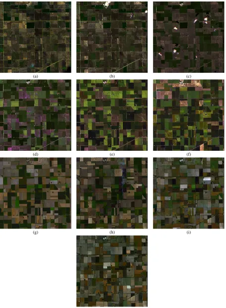
Experimental analyses were conducted using SITS data composed of atmospherically corrected and ortho-rectified RapidEye images. These images were acquired with the spatial resolution of 6.5 m at 10 different dates, during 2012 growing season from southwest of Winnipeg, Manitoba, Canada (see Table 1 for dates of acquisition). These images were collected to support the calibration/validation campaign of NASA’s soil moisture mission (Soil Moisture Active-Passive satellite: SMAP) (McNairn et al., 2015). In this study, the images were resampled to the spatial resolution of 10 m. After resampling, each image has the dimension of 1500×1500 pixels.
Figure 1. Block diagram of the proposed spatio-temporal feature extraction algorithm
In the experiments, we selected 70 fields of 6 different dominating crops in this region. For each crop, one of the fields was randomly selected as the training field, from which the training samples were again randomly selected. In addition, 3000 samples were randomly selected from all the fields of each crop as the testing samples. The crop types used for the crop mapping, their respective number of available fields, as well as the number of their training and testing samples are tabulated in Table 2. Figure 2 shows the true color composites of different images used in the experiments.
3.2 Experimental setup
Two different experiments were conducted to evaluate the effectiveness of the proposed spatio-temporal features for crop mapping. The goal of the first experiment is to analyze how the polynomial degree affects the classification accuracy of the proposed spatio-temporal features. In this experiment, the spatio-temporal features, extracted by considering different values for the polynomial degrees, were classified and compared based on their classification accuracies. We selected the polynomial degrees from the range of 2 to 6 with an increment step size of 1.
aimed
The second experiment to compare the
proposed spatio
classification results of the -temporal
features with those obtained using the other spatial and temporal features. The following features were considered for comparison in this experiment:
Raw values of vegetation index time-series. These values can be considered as temporal features.
Mean and homogeneity features estimated from gray level co-occurrence matrix (GLCM) were extracted from VI-SITS data, as spatial features. These features, represented as GLCM-mean and GLCM-Homogeneity, were calculated by varying the spatial window size in a range [5-21] an increment step size of 2.
As another spatio-temporal feature, an image segmentation algorithm was used to obtain the segments and then the phenological metrics were extracted from each segment. Area under profiles,
occurrence of
time
their respective , and the
amplitude of index are considered as the phenological metrics. These features are denoted as spatio-temporal phenology features.
In order to obtain image segments in both experiments, we used the multiresolution image segmentation algorithm which has three open parameters, namely scale, shape, and compactness (Benz et al., 2004). In the experiments, we set the values of these parameters to 5, 0.05 and 0.5 respectively. These values were obtained through trying different sets of values for these parameters and selecting the best one based on the visual comparison of the results.
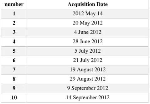
Table 1. Acquisition dates of different RapidEye images
number Acquisition Date
1 2012May14
2 20 May 2012
3 4 June 2012
4 28 June 2012
5 5 July 2012
6 21 July 2012
7 19 August 2012
8 29 August 2012
9 9 September 2012
10 14 September 2012
Table 2. Number of fields and samples per crop used for training and testing
Class Number
No Name Fields Training Testing
1 Corn 6 312 3000
2 Canola 15 673 3000
3 Wheat 15 597 3000
4 Soy 15 635 3000
5 Oat 15 290 3000
6 Sunflower 4 320 3000
111
(a) (b) (c)
(d) (e) (f)
(g) (h) (i)
(j)
Although all classification algorithms can be used for classifying the proposed features, in this paper we used support vector machines (SVM) as classification algorithm. The SVM algorithm was selected due to its theoretical properties and its proven empirical effectiveness ( Camps-Valls & Bruzzone, 2005; Mountrakis et al., 2011). To implement the SVM algorithm, the radial basis function (RBF) was considered as the kernel function. The RBF kernel parameter was tuned in the range [0.01-10] with a step size of 0.5 by using a 5-fold cross-validation. Furthermore, the trade-off parameter of the SVM algorithm was also selected from the range [0.1-2000] with an increment step size of 100 by using a 5-fold cross-validation.
4. Experimental Result
4.1 Effects of polynomial degree on the accuracy of crop mapping
In this experiment, the performances of the proposed spatio-temporal features were evaluated by considering polynomial functions with different degrees. To this end, we initially estimated the root mean square error (RMSE) of the fitted polynomials with different degrees to both time-series. The obtained RMSE values are shown in Figure 3.
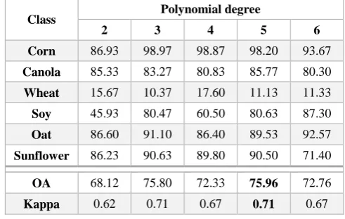
The obtained classification accuracies in term of overall accuracy, kappa coefficient and class accuracies are shown in Table 3 and Table 4 for NDVI and SAVI time-series respectively. Based on these tables, the obtained results were unsatisfactory in the case of considering a polynomial of small degree (e.g., 2, 3). As an example, classification of the spatio-temporal features extracted from SAVI and NDVI time-series considering a second-degree polynomial yielded the accuracy of 68.12% and 72.63%, respectively. By increasing the degree of polynomial, the classification performances of the features increases, until it reached its maximum at 87.93% and 75.96% for NDVI and SAVI time-series respectively using the fifth-degree polynomial. By further increasing the polynomial degree, a sharp decrease was observed in the classification actuaries. This is due to the fact that by increasing the polynomial degree, the possibility of overfitting increases. Thus, in spite of having a very small RMSE, the fitted polynomial cannot correctly model the time-series profiles.
Since the time-series profiles are usually very complex, finding the best polynomial degree to correctly fit the data is not a straightforward task. Furthermore, the presence of noise in the data makes this issue even more challenging. However, the polynomial functions with small degrees are always preferred over those with higher degrees, because of their lower probability of overfitting.
For a comparison, we showed the average values of NDVI time-series profiles of different crops and their fitted
average values at certain times during their growing season. Regarding the obtained accuracy of different crops, it is observable that wheat was the most challenging crop to classify, and in comparison to other crops, its accuracy was more affected by the polynomial degree. The results also showed that the NDVI time-series always yielded higher classification accuracy than the SVAI time-series.
Figure 3. Obtained RMSE of fitted polynomial functions with different degrees to both time-series
Table 3. Overall accuracy (OA), class accuracy and the kappa coefficient obtained from NDVI SITS using the proposed spatio-temporal features by considering different degrees for polynomials
Class Polynomial degree
2 3 4 5 6
Corn 69.70 80.07 87.00 84.73 82.20
Canola 99.70 92.40 95.67 99.87 95.67
Wheat 28.57 48.37 43.73 84.30 53.33
Soy 52.23 82.13 77.77 79.47 82.50
Oat 89.43 86.50 80.07 81.30 94.23
Sunflower 96.17 97.83 96.77 97.93 97.67
OA 72.63 81.22 80.17 87.93 84.27
Kappa 0.67 0.77 0.76 0.85 0.81
Table 4. Overall accuracy (OA), class accuracy and the kappa coefficient obtained from SAVI SITS using the proposed spatio-temporal features by considering different degrees for polynomials
Class Polynomial degree
2 3 4 5 6
Corn 86.93 98.97 98.87 98.20 93.67
Canola 85.33 83.27 80.83 85.77 80.30
Wheat 15.67 10.37 17.60 11.13 11.33
Soy 45.93 80.47 60.50 80.63 87.30
Oat 86.60 91.10 86.40 89.53 92.57
111 4.2 Comparison between different features
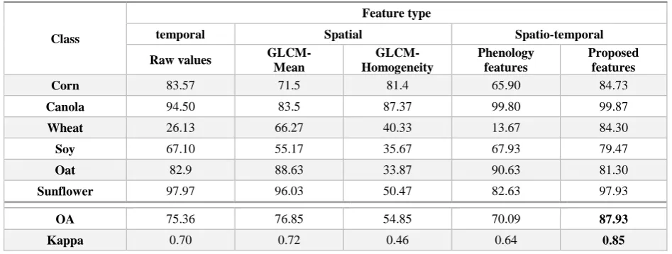
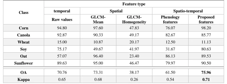
This experiment tries to compare the obtained accuracy of the proposed spatio-temporal features for crop mapping with those of the other features. Table 5 and Table 6 show the obtained results of crop mapping by considering various features. These tables also show the best-obtained accuracy from the classification of the proposed spatio-temporal features from the previous experiment.
As shown in these tables, the proposed spatio-temporal features due to proper modeling of both spatial and temporal patterns of the time-series data yielded much higher accuracies in comparison with the other features.
Here, the raw values of the time-series were considered as the temporal features. It can be seen that these features yielded the accuracy of 75.36% and 70.76% for NDVI and SAVI time-series respectively. By including the spatial features of GLCM-mean, the performance of the
classification showed a marginal improvement. However, the GLCM-Homogeneity by providing 54.85% and 38.17% for classification accuracy showed very weak performances. The weak results obtained from the GLCM-homogeneity features is due to the fact that the crop fields in this area are very homogenous, so they cannot be discriminated considering their homogeneity levels which are estimated by GLCM-homogeneity feature.
The spatio-temporal phenology features showed weaker results in comparison with the temporal features. This may happen due to the strong correlation between the phonological features extracted from image segments by the time-series values of the segments.
In this experiment, the NDVI time-series always provided higher classification accuracies than the SAVI time-series regardless of the used features.
Figure 4. Average value of NDVI for different crops and the fitted polynomial functions
Table 5. Overall accuracy (OA), class accuracy and the kappa coefficient obtained from crop mapping by considering different features extracted from NDVI SITS
Class
Feature type
temporal Spatial Spatio-temporal
Raw values GLCM- Mean
GLCM-Homogeneity
Phenology features
Proposed features
Corn 83.57 71.5 81.4 65.90 84.73
Canola 94.50 83.5 87.37 99.80 99.87
Wheat 26.13 66.27 40.33 13.67 84.30
Soy 67.10 55.17 35.67 67.93 79.47
Oat 82.9 88.63 33.87 90.63 81.30
Sunflower 97.97 96.03 50.47 82.63 97.93
OA 75.36 76.85 54.85 70.09 87.93
Table 6. Overall accuracy (OA), class accuracy and the kappa coefficient obtained from crop mapping by considering different features extracted from SAVI SITS
Class
Feature type
temporal Spatial Spatio-temporal
Raw values GLCM- Mean
GLCM-Homogeneity
Phenology features
Proposed features
Corn 94.80 97.60 47.83 76.07 98.20
Canola 92.87 90.33 49.17 82.67 85.77
Wheat 15.00 10.87 20.17 12.50 11.13
Soy 75.17 49.67 41.97 31.67 80.63
Oat 57.07 96.40 23.40 86.13 89.53
Sunflower 89.63 95.00 46.47 79.97 90.50
OA 70.76 73.31 38.17 61.50 75.96
Kappa 0.65 0.68 0.26 0.54 0.71
Based on the results wheat and soy showed the lowest class accuracies by use of different features. The highest class accuracy of these two crops was obtained by the proposed spatio-temporal features from the NDVI time series, which was 84.30% for wheat and 79.47% for soy. For a qualitative analysis, Figure 5 shows the obtained crop maps by considering raw NDVI values and the proposed spatio-temporal features. As shown in Figure 5, the obtained crop maps of the proposed spatio-temporal feature are not only more accurate but also, due to use of the spatial information, are smoother than the crop map obtained from raw time-series values.
5. Conclusion
Time-series data constructed from the images of sensors with high spatial resolution and short revisit times can provide very valuable information regarding spatial and temporal patterns of crops during their growing cycles. This information, if properly extracted, can be used for producing accurate crop maps. In this paper, we proposed a new algorithm for extracting spatio-temporal features from time-series of vegetation indices. The proposed algorithm consists of two steps. In the first step, the spatial patterns of the time-series data are modeled using an image segmentation method. In the second step, a polynomial function is fitted to the average value of the pixels belong to each segment and its coefficients are used as the spatio-temporal features.
The obtained results of our experiments showed that the
proposed spatio-temporal features, due to their ability to extract and model both the spatial and the temporal patterns of the time-series data, can provide higher classification accuracy for crop mapping in comparison to common temporal, spatial and spatio-temporal features.
In addition, based on the results, it can be concluded that polynomial functions can properly be exploited as the temporal features. However, the polynomial degree highly affects the classification performance of these features. Using a low degree polynomial may fail to correctly model time-series profiles. However, increasing the degree may increase the chance of overfitting.
Despite the promising results of the proposed spatio-temporal features in this study, there are some issues that need to be studied further. Evaluating the performance of other functions such as splines for modeling the time-series profiles and the use of meta-heuristic optimization methods for optimizing the polynomial degree are amongst these issues.
Acknowledgment
121
(a) (b) (c)
Corn canola wheat soy oat sunflower
Figure5.Crop maps obtained through theclassification of different features of NDVI time-series (a) Raw values; (b) proposed spatio-temporal feature; and (c) testing fields
References
Ali, M., Montzka, C., Stadler, A., Menz, G., Thonfeld, F., & Vereecken, H. (2015). Estimation and validation of RapidEye-based time-series of leaf area index for winter wheat in the Rur catchment (Germany). Remote sensing, 7(3), 2808-2831. Bach, H., Friese, M., Spannraft, K., Migdall, S., Dotzler, S., Hank,
T., . . . Mauser, W. (2012). Integrative use of multitemporal RapidEye and Terrasar-X data for agricultural monitoring. Paper presented at the 2012 IEEE International Geoscience and Remote Sensing Symposium, Munich, Germany
Benz, U. C., Hofmann, P., Willhauck, G., Lingenfelder, I., & Heynen, M. (2004). Multi-resolution, object-oriented fuzzy analysis of remote sensing data for GIS-ready information.
ISPRS Journal of Photogrammetry and Remote Sensing, 58(3), 239-258.
Camps-Valls, G., & Bruzzone, L. (2005). Kernel-based methods for hyperspectral image classification. IEEE Transactions on Geoscience and Remote Sensing, 43(6), 1351-1362.
Daya Sagar, B. S., & Serra, J. (2010). Spatial information retrieval, analysis, reasoning and modelling. International Journal of Remote Sensing, 31(22), 5747-5750. doi: 10.1080/01431161.2010.512315
Definiens, A. (2009). Definiens eCognition developer 8 user guide.
Definens AG, Munchen, Germany.
DeFries, R., Hansen, M., & Townshend, J. (1995). Global discrimination of land cover types from metrics derived from AVHRR pathfinder data. Remote sensing of environment, 54(3), 209-222.
Geerken, R., Zaitchik, B., & Evans, J. (2005). Classifying rangeland vegetation type and coverage from NDVI time series using Fourier Filtered Cycle Similarity. International Journal of Remote Sensing, 26(24), 5535-5554.
Gerstmann, H., Möller, M., & Gläßer, C. (2016). Optimization of spectral indices and long-term separability analysis for classification of cereal crops using multi-spectral RapidEye imagery. International Journal of Applied Earth Observation and Geoinformation, 52, 115-125.
Hill, M. J., & Donald, G. E. (2003). Estimating spatio-temporal patterns of agricultural productivity in fragmented landscapes using AVHRR NDVI time series. Remote sensing of environment, 84(3), 367-384.
Huete, A. R. (1988). A soil-adjusted vegetation index (SAVI).
Remote sensing of environment, 25(3), 295-309. doi:
http://dx.doi.org/10.1016/0034-4257(88)90106-X
Jackson, R. D. (1986). Remote sensing of biotic and abiotic plant stress. Annual review of phytopathology, 24(1), 265-287.
Jamali, S., Seaquist, J., Eklundh, L., & Ardö, J. (2014). Automated mapping of vegetation trends with polynomials using NDVI imagery over the Sahel. Remote sensing of environment, 141, 79-89.
Jonsson, P., & Eklundh, L. (2004). TIMESAT - a program for analyzing time-series of satellite sensor data. Computers & Geosciences, 30, 833-845.
Julea, A., Méger, N., Rigotti, C., Trouvé, E., Jolivet, R., & Bolon, P. (2012). Efficient Spatio-temporal Mining of Satellite Image Time Series for Agricultural Monitoring. Trans. MLDM, 5(1), 23-44.
Kross, A., McNairn, H., Lapen, D., Sunohara, M., & Champagne, C. (2015). Assessment of RapidEye vegetation indices for estimation of leaf area index and biomass in corn and soybean crops. International Journal of Applied Earth Observation and Geoinformation, 34, 235-248.
Li, Q., Cao, X., Jia, K., Zhang, M., & Dong, Q. (2014). Crop type high
integration of by
identification -spatial resolution from coarse extracted
multispectral data with features -resolution time-series vegetation index data. International Journal of Remote Sensing, 35(16), 6076-6088.
Löw, F., Conrad, C., & Michel, U. (2015). Decision fusion and non-parametric classifiers for land use mapping using multi-temporal RapidEye data. ISPRS Journal of Photogrammetry and Remote Sensing, 108, 191-204.
McNairn, H., Jackson, T. J., Wiseman, G., Bélair, S., Berg, A., Bullock, P., . . . Hosseini, M. (2015). The Soil Moisture Active Passive Validation Experiment 2012 (SMAPVEX12): Pre-Launch Calibration and Validation of the SMAP Soil Moisture Algorithms. IEEE Trans. Geosci. Remote Sens, 53(5). Meroni, M., Verstraete, M. M., Rembold, F., Urbano, F., &
Kayitakire, F. (2014). A phenology-based method to derive biomass production anomalies for food security monitoring in the Horn of Africa. International Journal of Remote Sensing, 35(7), 2472-2492.
Mirik, M., Ansley, R., Michels Jr, G., & Elliott, N. (2012). Spectral vegetation indices selected for quantifying Russian wheat aphid (Diuraphis noxia) feeding damage in wheat (Triticum aestivum L.). Precision Agriculture, 13(4), 501-516.
Mountrakis, G., Im, J., & Ogole, C. (2011). Support vector machines in remote sensing: A review. ISPRS Journal of Photogrammetry and Remote Sensing, 66(3), 247-259. Niazmardi, S., Homayouni, S., Safari, A., Shang, J., & McNairn, H.
(2018). Multiple kernel representation and classification of multivariate satellite-image time-series for crop mapping.
International Journal of Remote Sensing, 39(1), 149-168. Pan, Z., Huang, J., Zhou, Q., Wang, L., Cheng, Y., Zhang, H., . . .
time-series derived from HJ-1 A/B data. International Journal of Applied Earth Observation and Geoinformation, 34(Supplement C), 188-197. doi:
https://doi.org/10.1016/j.jag.2014.08.011
Prasad, A. K., Chai, L., Singh, R. P., & Kafatos, M. (2006). Crop yield estimation model for Iowa using remote sensing and surface parameters. International Journal of Applied Earth Observation and Geoinformation, 8(1), 26-33.
Rouse Jr, J. W., Haas, R., Schell, J., & Deering, D. (1974). Monitoring vegetation systems in the Great Plains with ERTS.
NASA special publication, 351, 309.
Simonneaux, V., Duchemin, B., Helson, D., Er‐Raki, S., Olioso, A., & Chehbouni, A. G. (2008). The use of high‐resolution image time series for crop classification and evapotranspiration estimate over an irrigated area in central Morocco. International Journal of Remote Sensing, 29(1), 95-116. doi: 10.1080/01431160701250390
Spruce, J. P., Sader, S., Ryan, R. E., Smoot, J., Kuper, P., Ross, K., . . . McKellip, R. (2011). Assessment of MODIS NDVI time series data products for detecting forest defoliation by gypsy moth outbreaks. Remote sensing of environment, 115(2), 427-437.
Verhegghen, A., Bontemps, S., & Defourny, P. (2014). A global NDVI and EVI reference data set for land-surface phenology using 13 years of daily SPOT-VEGETATION observations.
International Journal of Remote Sensing, 35(7), 2440-2471. Wagenseil, H., & Samimi, C. (2006). Assessing spatio‐temporal
variations in plant phenology using Fourier analysis on NDVI time series: results from a dry savannah environment in Namibia. International Journal of Remote Sensing, 27(16), 3455-3471.