https://doi.org/10.5194/gmd-12-2523-2019 © Author(s) 2019. This work is distributed under the Creative Commons Attribution 4.0 License.
Vertically nested LES for high-resolution simulation of
the surface layer in PALM (version 5.0)
Sadiq Huq1, Frederik De Roo1,4, Siegfried Raasch3, and Matthias Mauder1,2
1Institute of Meteorology and Climate Research, Atmospheric Environmental Research (IMK-IFU), Karlsruhe Institute of Technology (KIT), Kreuzeckbahnstrasse 19, 82467 Garmisch-Partenkirchen, Germany
2Institute of Geography and Geoecology (IfGG), Karlsruhe Institute of Technology, Kaiserstrasse 12, 76131 Karlsruhe, Germany
3Institute of Meteorology and Climatology, Leibniz Universität Hannover, Hanover, Germany 4Norwegian Meteorological Institute, Oslo, Norway
Correspondence:Matthias Mauder ([email protected]) Received: 15 November 2018 – Discussion started: 3 December 2018 Revised: 16 April 2019 – Accepted: 4 June 2019 – Published: 28 June 2019
Abstract.Large-eddy simulation (LES) has become a well-established tool in the atmospheric boundary layer research community to study turbulence. It allows three-dimensional realizations of the turbulent fields, which large-scale mod-els and most experimental studies cannot yield. To resolve the largest eddies in the mixed layer, a moderate grid resolu-tion in the range of 10 to 100 m is often sufficient, and these simulations can be run on a computing cluster with a few hundred processors or even on a workstation for simple con-figurations. The desired resolution is usually limited by the computational resources. However, to compare with tower measurements of turbulence and exchange fluxes in the sur-face layer, a much higher resolution is required. In spite of the growth in computational power, a high-resolution LES of the surface layer is often not feasible: to fully resolve the energy-containing eddies near the surface, a grid spacing of O(1 m) is required. One way to tackle this problem is to em-ploy a vertical grid nesting technique, in which the surface is simulated at the necessary fine grid resolution, and it is cou-pled with a standard, coarse, LES that resolves the turbulence in the whole boundary layer. We modified the LES model PALM (Parallelized Large-eddy simulation Model) and im-plemented a two-way nesting technique, with coupling in both directions between the coarse and the fine grid. The cou-pling algorithm has to ensure correct boundary conditions for the fine grid. Our nesting algorithm is realized by mod-ifying the standard third-order Runge–Kutta time stepping to allow communication of data between the two grids. The
two grids are concurrently advanced in time while ensuring that the sum of resolved and sub-grid-scale kinetic energy is conserved. We design a validation test and show that the tem-porally averaged profiles from the fine grid agree well com-pared to the reference simulation with high resolution in the entire domain. The overall performance and scalability of the nesting algorithm is found to be satisfactory. Our nesting re-sults in more than 80 % savings in computational power for 5 times higher resolution in each direction in the surface layer.
1 Introduction
e.g., Deardorff (1974), Moeng and Wyngaard (1988) and Schmidt and Schumann (1989), where the presence of a sub-grid-scheme allows that only the most energetic eddies are resolved. One of the first large-eddy simulations (LESs) by Deardorff (1974) used 64 000 grid points to simulate a domain of 5 km×5 km×2km with a grid resolution of (125,125,50)m. The size of one such grid cell is just suf-ficient to resolve the dominant large eddies, and there are just enough grid points to represent the ABL. As computing power progressed, higher resolution and larger domains be-came possible. By the time of Schmidt and Schumann (1989) the number of grid cells had risen to 160×160×48, simu-lating an ABL of 8 km×8 km×2.4 km with a resolution of (50,50,50)m. Khanna and Brasseur (1998) used 1283grid points to simulate a domain of 3 km×3 km×1 km to study buoyancy and shear-induced local structures of the ABL. Pat-ton et al. (2016) used (2048,2048,1024) grid points with a grid resolution of(2.5,2.5,2)m to study the influence of atmospheric stability on canopy turbulence. More recently, Kröniger et al. (2018) used 13×109grid points to simulate a domain of 30.72 km×15.36 km×2.56 km to study the influ-ence of stability on the surface–atmosphere exchange and the role of secondary circulations in the energy exchange. The atmospheric boundary layer community has greatly bene-fited from the higher spatial resolution available in these LES to study turbulent processes that cannot be obtained in field measurements. Still, especially in heterogeneous terrain, near topographic elements and buildings or close to the surface, the required higher resolution is not always attainable due to computational constraints. In spite of the radical increase in the available computing power over the last decade, large-eddy simulation of high Reynolds number atmospheric flows with very high resolution in the surface layer remains a chal-lenge. Considering the size of the domain required to repro-duce boundary-layer-scale structures, it is computationally demanding to generate a single fixed grid that could resolve all relevant scales satisfactorily. Alternatively, local grid re-finement is possible in the finite volume codes that are not restricted to structured grids. Flores et al. (2013) developed a solver for the OpenFOAM modeling framework to sim-ulate atmospheric flows over complex geometries using an unstructured mesh approach. The potential of the adaptive mesh refinement technique in which the tree-based Cartesian grid is refined or coarsened dynamically, based on the flow structures, is demonstrated by van Hooft et al. (2018). In the finite difference models, a grid nesting technique can be em-ployed to achieve the required resolution. In the nested grid approach, a parent domain with a coarser resolution simu-lates the entire domain, while a nested grid with a higher res-olution extends only up to the region of interest. Horizontal nesting has been applied to several mesoscale models (Ska-marock et al., 2008; Debreu et al., 2012). Horizontally nested LES-within-LES or LES embedded within a mesoscale sim-ulation is available in the Weather Research and Forecast model (Moeng et al., 2007). Comparable grid nesting
tech-niques are also widely employed by the engineering turbu-lence research community but often use different terminol-ogy. Nesting in codes with Cartesian grids is referred to as local or zonal grid algorithm (Kravchenko et al., 1996; Boersma et al., 1997; Manhart, 2004) and as overset mesh (Nakahashi et al., 2000; Kato et al., 2003; Wang et al., 2014) in unstructured or moving grid codes.
For our purposes, we will focus on vertical nesting; i.e., we consider a fine grid nested domain (FG) near the lower boundary of the domain and a coarse grid parent domain (CG) in the entirety of the boundary layer. While the lat-ter’s resolution (<50 m) is sufficient to study processes in the outer region where the dominant eddies are large and in-ertial effects dominate, such coarse resolution is not suffi-cient where fine-scale turbulence in the surface layer region is concerned. The higher resolution achieved by the vertical nesting will then allow a more accurate representation of the turbulence in the surface layer region, by resolving its domi-nant eddies. For studies that require very high resolution near the surface (e.g., virtual tower measurements, wakes behind obstacles, dispersion within street canyons for large cities), a nesting approach is an attractive solution due to the reduced memory requirement. A challenge of the vertically nested simulation is that the FG upper boundary conditions need to be correctly prescribed by the CG. Though vertical nesting is less common than the horizontal nesting, it has been im-plemented in some LES models. A non-parallelized vertical nesting was explored by Sullivan et al. (1996), but the code is not in the public domain, and we could not find any record of further development or application of this code in publi-cations. A LES-within-LES vertical nesting is implemented by Zhou et al. (2018) in the Advanced Regional Prediction System (ARPS) model. We would like to point out that the vertical nesting available in the Weather Research and Fore-cast model (Daniels et al., 2016) is not a conventional ver-tical nesting because the parent and the child grid still have the same vertical extent; the child grid is only more refined in the vertical.
and Hall (1991) studied two different approaches for updat-ing the CG values, namely “post-insertion” and “pressure de-fect correction”. The two approaches were also investigated by Sullivan et al. (1996) in their vertical nesting implementa-tion. In the post-insertion technique, once the Poisson equa-tion for pressure is solved in the FG, the resolved fields are then anterpolated to the CG. In the pressure defect correc-tion approach, the pressure in the CG and FG are matched by adding a correction term to the CG momentum equations, and an anterpolation operation is not required. Though Sulli-van et al. (1996) note the pressure defect correction approach to be more elegant, no significant difference in the results was reported. In the following sections we describe the technical realization and numerical aspects of the two-way nesting al-gorithm. In the LES model PALM, a validation simulation is set up, and the results of the nested and stand-alone simula-tions are compared. A second simulation is set up to evaluate the computational performance of the algorithm. The practi-cal considerations and the limitations of the two-way nesting are then discussed.
2 Methods
2.1 Description of the standard PALM
The Parallelized Large-eddy simulation Model (PALM) is developed and maintained at the Leibniz University of Hanover (Raasch and Schröter, 2001; Maronga et al., 2015). We give a quick summary of the model here and highlight the aspects which will reappear when discussing our nest-ing modifications. PALM is a finite difference solver for the non-hydrostatic incompressible Navier–Stokes equations in the Boussinesq approximation. PALM solves for six prog-nostic equations: the three components of the velocity field (u, v, w), potential temperature (θ), humidity (q) and the sub-grid-scale kinetic energy (e). The sub-grid-scale (SGS) tur-bulence is modeled based on the method proposed by Dear-dorff (1980). The equations for the conservation of mass, energy and moisture (Eqs. 1, 2, 3 and 4) are filtered over a grid volume on a Cartesian grid. Adopting the convention of Maronga et al. (2015), the overbar denoting the filtered variables is omitted. However, the overbar is shown for SGS fluxes. The SGS variables are denoted by a double prime. The prognostic equations for the resolved variables are
∂ui ∂t = −
∂uiuj ∂xj
−εij kfjuk+εi3kf3ukg,j−
1 ρ0
∂π∗ ∂xi
+gθv− hθvi θv
δi3− ∂ ∂xj
u00iu00j−2 3eδij
, (1)
∂uj ∂xj
=0, (2)
∂θ ∂t = −
∂ujθ ∂xj
− ∂ ∂xk
u00jθ00− LV
cp5
9qv, (3)
∂qv ∂t = −
∂ujqv ∂xj
− ∂ ∂xk
u00jq00
v
+9qv. (4)
The symbols used in the above equations are listed in Table 1. The 1.5-order closure parameterization modified by Moeng and Wyngaard (1988) and Saiki et al. (2000) assumes a gradi-ent diffusion parameterization (Eqs. 6, 7, 8). The prognostic equation for the SGS turbulent kinetic energy (TKE) reads as ∂e
∂t = −uj ∂e ∂xj
−u00iu00j∂ui ∂xk
+ g θv,0
u003θ00
v−2Km ∂e ∂xj
− , (5) with the SGS fluxes modeled as
u00iu00j−2
3eδij= −Km ∂u
i ∂xj
+∂uj ∂xi
, (6)
u00iθ00= −K
h ∂θ ∂xi
(7) and
u00iq00
v = −Kh ∂θ ∂xi
. (8)
The eddy diffusivities are proportional toe3/2under convec-tive conditions (Maronga et al., 2015). For a thorough de-scription of the governing equations and parameterizations, see Maronga et al. (2015).
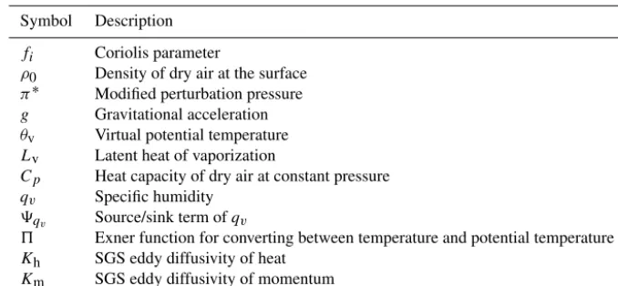
Table 1.List of symbols in the governing equations and parameterizations.
Symbol Description
fi Coriolis parameter
ρ0 Density of dry air at the surface π∗ Modified perturbation pressure g Gravitational acceleration θv Virtual potential temperature Lv Latent heat of vaporization
Cp Heat capacity of dry air at constant pressure qv Specific humidity
9qv Source/sink term ofqv
5 Exner function for converting between temperature and potential temperature Kh SGS eddy diffusivity of heat
Km SGS eddy diffusivity of momentum
zero at both top and bottom boundaries. PALM is a paral-lelized model, and the standard way of parallelization is by dividing the three-dimensional domain into vertical columns, each of which is assigned to one processing element (PE). Each vertical column possesses a number of ghost points needed for computation of derivatives at the boundary of the domains. Each PE can only access data for a single sub-domain. All PEs execute the same program on a different set of data. For optimum load balancing between the PEs, the decomposed sub-domains should have the same size. In PALM, this condition is always satisfied as only sub-domains of the same size are allowed. The data exchange between PEs needed by the Poisson solver and to update the ghost points is performed via the Message Passing Interface (MPI) com-munication routines.
2.2 Nested model structure
2.2.1 Fine grid and coarse grid configuration
We are interested in achieving an increased resolution only in the surface layer, the lowest 10 % of the boundary layer, where surface exchange processes occur and where eddies generated by surface heterogeneity and friction are smaller than the dominant eddies in the mixed layer. We set up the LES-within-LES case by maintaining the same horizontal extent for the FG and the CG to have the whole surface better resolved. We allow the vertical extent of the FG to be var-ied as needed, typically up to the surface layer height. This implementation of vertical grid nesting has two main chal-lenges. The first challenge, that is purely technical in nature, is to implement routines that handle the communication of data between the CG and the FG. The second and the most important challenge is to ensure that the nesting algorithm yields an accurate solution in both grids. Below we use up-per case symbols for fields and variables in the CG and lower case for the FG; e.g.,Eandedenote the sub-grid-scale turbu-lent kinetic energy (a prognostic variable in our LES) of CG
and FG respectively. The nesting ratio is defined as the ratio of the CG spacing to the FG spacing, andnx=1X/1x;
cor-responding symbols apply foryandzdirections. The nesting ratiosnx,nyandnzhave to be integers. It is possible to have
either an odd or even nesting ratio, and it can be different in each direction. As the domain that is simulated in the FG is completely inside of the CG domain, each FG cell belongs to a CG cell. The two grids are positioned in such a way that a FG cell belongs to only one CG cell, and one CG cell is made up by a number of FG cells given by the product of the nesting ratiosnx×ny×nz. This means that if the grid nesting
ratio is odd, there will be one FG cell whose center is exactly at the same position as the center of the coarse cell as shown in Fig. 1b. The collection of FG cells that correspond to one CG cell is denoted byC(I, J, K). The collection ofyzfaces of the FG that corresponds to ayzface of the CG is denoted byCx(Is, J, K), where it is understood that theIsindex is an index on the staggered grid in thex direction to denote the position of the face, and this is similar for the other types of faces. We have usedfx=1/nx to denote the inverse of the
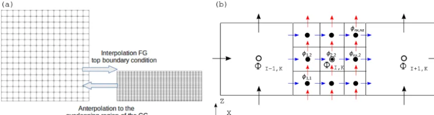
nesting ratio in thex dimension (corresponding symbols for y andz). A schematic diagram of the overlapping grids is shown in Fig. 1a.
2.2.2 Vertical nesting algorithm
Figure 1. (a)Schematic of the interpolation and anterpolation between grids. The FG top boundary condition is interpolated from the CG. The CG prognostic quantities in the overlapping region are anterpolated from the FG.(b)Schematic of Arakawa C grid for two grids with nesting ratio of 3. The black arrows and circles are CG velocity and pressure, respectively. The blue and red arrows are horizontal and vertical velocity, respectively, in the FG. The filled black circle is the FG pressure. The symbols8andφrepresent CG and FG scalar quantities.I andKare CG indices andnxandnzare the nesting ratio inxandz, respectively.
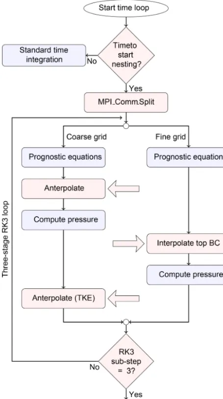
the prognostic equation except for the pressure is first com-puted concurrently in both grids. The values ofu, v, w, θand q are then anterpolated to the CG in the overlapping region. The CG solves a Poisson equation for pressure. The new u, v, w, θ andq fields in the CG are interpolated to set the FG Dirichlet top boundary conditions. The Poisson equation is then solved for pressure in the FG, and the vertical velocity in the FG is also updated by the pressure solver at this stage. Since all the velocity components follow a Dirichlet condi-tion at the FG top boundary, only a Neumann condicondi-tion is suitable for pressure (Manhart, 2004). PALM permits the use of a Neumann zero-gradient condition for pressure at both the top and bottom boundary. It is advisable to use a Neu-mann boundary condition at the top and the bottom for the CG too. The TKE is then anterpolated maintaining the Ger-mano identity, and it is followed by the computation of SGS eddy diffusivity for heat (kh) and momentum (km) in the CG. This procedure is repeated at every sub-step of the Runge– Kutta 3 time integration, and it ensures that the velocity field remains divergence free in both grids.
In the 1.5-order turbulence closure parameterization, all the sub-grid fluxes are derived from the turbulent kinetic en-ergy and the resolved gradients at each time step. Therefore, the sub-grid fluxes do not have to be interpolated from CG to FG at the top boundary. Furthermore, in our implementa-tion of the nesting method, we assume that most of the TKE is resolved well down to the inertial subrange, except for the lowest few grid layers. This allows us to use the zero-gradient Neumann boundary condition for TKE at the FG top bound-ary. We employ a simplified sponge layer by limiting the an-terpolation of all prognostic quantities to one CG cell fewer than the nested height. This segregation of the anterpolation region in the CG and top boundary condition level of the FG ensures that the flow structures in the CG propagate into the FG without distortion due to numerical artifacts.
2.3 Translation between grids 2.3.1 Interpolation
For the boundary conditions at the top of the FG, the fields from the CG are interpolated to the FG, according to Clark and Farley (1984). We define the top of the FG as the bound-ary level just above the prognostic level of each quantity. In Eq. (10),8andφ represent CG and FG quantities, respec-tively. For the scalar fields, the interpolation is quadratic in all three directions. For the velocity components, the inter-polation is linear in its own dimension and quadratic in the other two directions. The same interpolation formulation is also used to initialize all vertical levels of the fine grid do-main at the beginning of the nested simulation. The interpo-lation is reversible as it satisfies the conservation condition of Kurihara et al. (1979):
< φ >=< 8 > . (9)
For clarity, we illustrate the interpolation by focusing on one particular dimension, in this casex, but the same operation holds foryandz. The interpolation in thexdimension reads as
φm=ηm−8I−1+η0m8I+ηm+8I+1, (10) withmrunning from 1 tonx, thus producingnx equations
for each CG cellI. For the interpolation inyandzthere will be two additional indices, producingnx×ny×nzequations
Figure 2.A flowchart of the two-way interaction algorithm. The new routines needed for the vertical nesting are highlighted in red and the standard routines are highlighted in blue. An arrow pointing to the left indicates transfer of data from FG to CG, and vice versa.
ηm−=
1
2Hm(Hm−1)+α, ηm0 =(1−Hm2)−2α, ηm+=1
2Hm(Hm+1)+α ,
(11)
with the weights Hm expressed in function of the inverse
nesting ratio,
Hm=
1
2((2m−1)fx−1) , (12)
and the coefficientα is chosen such that the conservation condition of Kurihara et al. (1979) is satisfied:
α= 1 24
fx2−1. (13)
It can be observed that the sum of theηs equals 1. 2.3.2 Anterpolation
The anterpolation of the prognostic quantities is performed by an averaging procedure according to Clark and Hall (1991). The anterpolation equations for the velocities read as
UI,J,K=< u>j,k= X
j,k∈CIJ K
ui∗,j,kfyfz,
VI,J,K=< v>i,k= X
i,k∈CIJ K
vi,j∗,kfxfz,
WI,J,K=< w>i,j = X
i,j∈CIJ K
wi,j,k∗fxfy.
(14)
For the scalars it is 8I,J,K= [φ]i,j,k=
X
i,j,k∈CIJ K
φi,j,kfxfyfz. (15)
Here the lower case indices only count over the fine grid cells that belong to that particular coarse grid cell. For each (I, J, K)tuple of a parent CG cell, there exists a setCIJ K
containing the(i, j, k) tuples of its corresponding children FG cells. To ensure that the nested PALM knows at all times which fine grid cells and coarse grid cells correspond, we compute this mapping for the FG and CG indices before starting the simulation, and we store it in the memory of the parallel processing element. In the Arakawa C grid dis-cretization that PALM uses, the scalars are defined as the spatial average over the whole grid cell, and therefore it is re-quired that the CG scalar is the average of the corresponding FG scalars in (Eq. 15). However, the velocities are defined at the faces of the cells in the corresponding dimension. There-fore in (Eq. 14) the CG velocity components are computed as the average over the FG values at the FG cells that cor-respond to the face of the CG cell, expressed byi∗,j∗,k∗ respectively.
However, the TKE in the CG differs from the FG value, due to the different resolution of grids. In the FG the SGS motions are weaker because the turbulence is better resolved. Therefore, TKE is anterpolated such that the sum of resolved kinetic energy and TKE (SGS kinetic energy) is preserved, by maintaining the Germano identity (Germano et al., 1991):
E= [e] +1 2
3 X
n=1
([unun] − [un][un]) . (16)
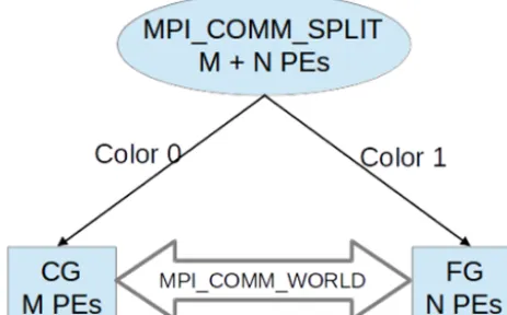
Figure 3.Schematic of the MPI processor grouping. The data ex-change between the two groups is performed via the global com-municator.MandN are the number of processors for CG and FG respectively.
over the three spatial dimensions. In other words, to obtain the CG TKE from the average FG TKE, we add the variance of the FG velocity components over the FG cells comprising the CG cell. Therefore CG TKE is always larger than FG TKE.
2.4 Parallel inter-grid communication
MPI is the most widely used large-scale parallelization library. The atmosphere–ocean coupling in PALM has been implemented following MPI-1 standards (Esau, 2014; Maronga et al., 2015). We follow a similar approach for the MPI communications and have adopted MPI-1 stan-dards for our nesting implementation. Concurrent execution of the two grids is achieved with the MPI_COMM_SPLIT procedure. The total available processors are split into two groups, denoted by color 0 or 1 for CG and FG respec-tively; see Fig. 3. The data between the processors of the same group are exchanged via the local communicator cre-ated during the splitting process, whereas the data between the two groups are exchanged via the global communicator MPI_COMM_WORLD.
Based on the nesting ratio and the processor topology of the FG and the CG group, a mapping list is created and stored. Given the local PE’s 2-D processor co-ordinate, the list will identify the PEs in the remote group to/from which data need to be sent/received; the actual communication then takes place via the global communicator. There are three types of communication in the nesting scheme:
i. Initialization of the FG. (Send data from coarse grid to fine grid.) This is performed only once.
ii. Boundary condition for the FG top face. (Send data
from coarse grid to fine grid.)
iii. Anterpolation. (Send data from fine grid to coarse grid.)
The exchange of arrays via MPI_SENDRECV routines is computationally expensive. Therefore, the size of the arrays communicated is minimized by performing the anterpolation operation in the FG PEs and storing the values in a tempo-rary 3-D array that is later sent via the global communica-tor to the appropriate CG PE. This approach is more effi-cient than performing the anterpolation operation on the CG which has fewer PEs and needs communication of larger ar-rays from the FG. Furthermore, the array data that need to be communicated during the anterpolation operation and for set-ting the FG boundary condition are not contiguous in mem-ory. The communication performance is enhanced by creat-ing an MPI-derived data type that ensures that the data are sent contiguously. Within the RK3 sub-steps, when one grid executes the pressure solver, the other grid has to wait, lead-ing to more computational time at every sub-step. However, the waiting time can be minimized by effective load balanc-ing; i.e., the number of grid points per PE in the CG should be kept lower than in the FG. The reduction in workload per CG PE is achieved with a few additional cores. The reduction in computational time per step in the CG means the waiting time on the FG PE is also reduced.
3 Results and discussion
temperature is initialized to a constant value of 300 K up to 800 m, and above 800 m a lapse rate of 1 K (100 m)−1is pre-scribed. The humidity profile is initialized to a constant value of 0.005 kg kg−1. The simulation is driven by prescribing a surface heat flux of 0.1 K m s−1and a surface humidity flux of 4×10⁻⁴kg kg−1m s−1. The domain is more than 4 times larger in the horizontal than the initial boundary layer height. 3.2 Analysis of the simulations
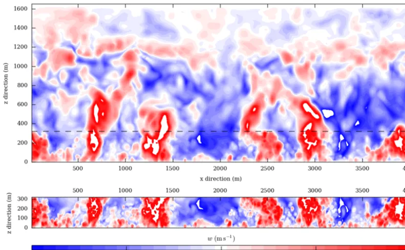
In a two-way nesting it is important that the flow structures are propagated from the FG to CG and vice versa, without any distortion. In Fig. 4, the contours in the CG region over-lapping the FG have similar structures as the FG. The higher resolution in the FG enables more detailed contours, whereas the anterpolated CG contours are smoother. Furthermore, in the CG region beyond the overlapping region, no distortion of the contours is observed, indicating that the anterpolation does not introduce sharp gradients in the CG.
Vertical profiles are used for quantitative comparison of the nested and the reference simulations. The turbulent fluc-tuations (e.g., θ00,w00) are defined as the spatial deviations from the instantaneous horizontal average. The turbulent fluxes (e.g., < w00θ00>, < u00u00>) are obtained using the
spatial covariance and are then horizontally averaged. All the horizontally averaged profiles (e.g., < θ >,< w00θ00>) are also averaged over time, but we omit the conventional over-line notation for readability. The convective velocity scale (w∗) and temperature scale (θ∗) obtained from SA-F are
used to normalize the profiles. The convective velocity is calculated asw∗=(g θ0−1Hs zi)1/3, wheregis the
gravita-tional acceleration,θ0is the surface temperature andziis the
boundary layer height in the simulation. The convective tem-perature scale is calculated asθ∗=Hs w∗−1. In Fig. 5a and c,
the vertical profiles of difference between the potential tem-perature (< θ >) and its surface value normalized by the con-vective temperature scale are plotted. Since the FG profiles are superior to the CG in the overlapping region, the anterpo-lated CG values are not plotted. In Fig. 5a, there is no visible difference between the stand-alone and the nested simula-tions. However, in the region closer to the surface, plotted in Fig. 5c, a better agreement between the SA-F and FG is ob-served. The potential temperature variance (< θ00θ00>) nor-malized by the square of the temperature scale (θ∗2) is shown
in Fig. 5b and d. Here too FG provides better accuracy close to the surface.
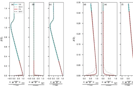
In the vertical heat flux (< w00θ00>) profiles in Fig. 6, the FG has good agreement with the SA-F in the surface layer for the resolved, SGS and the total flux profiles. In the CG regions above the nested grid height, a good agreement with the SA-C is found as well. The improvement due to the two-way nesting is seen in Fig. 6d and e, where the effects of low grid resolution of the SA-C in resolved and SGS fluxes are evident. However, no grid-dependent difference in the profile is observed in the total flux.
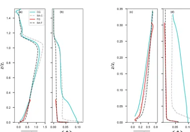
The resolved variances ofu,v andwnormalized by the square of the convective velocity (w2∗) are plotted in Fig. 7.
The FGvandwFG profiles have a better agreement with the SA-F than theuvariance. Theuandv variances in Fig. 7d and e lie between SA-C and SA-F, indicating that the re-solved variances are improved compared to the SA-C but not sufficiently resolved to match SA-F. At the nesting height the variances deviate more from the SA-F and approach the CG values. Due to conservation of total kinetic energy across the nest boundary, more CG TKE is contained in the sub-grid scale. Consequently, the resolved CG variances could have an undershoot as compared to SA-F, resulting in an under-shoot of the FG variances too at the nesting height. Above the nesting height, the variance ofu,vandwin CG is simi-lar to SA-C.
The resolved vertical velocity skewness in Fig. 8 shows good agreement between the FG and SA-F close to the sur-face. However, at the nesting height a small kink in the skew-ness is noticeable. Zhou et al. (2018) observe that the mag-nitude of the kink in the higher-order profiles can be mini-mized by increasing the depth of the sponge layer. Our sim-plified sponge layer approach appears to be unable to effec-tively minimize the kinks at the nesting height. The resolved skewness in CG is lower than SA-C, possibly due to larger SGS TKE in the CG, as seen in Fig. 8d. The SGS TKE in Fig. 8d shows an exact match between FG and SA-F close to the surface and only marginal difference at the nesting height. However, CG values are considerably different from the SA-C values close to the surface due to the anterpolation main-taining the Germano identity for conservation of kinetic en-ergy across the grids. In the coarse-resolution SA-C, near the surface, the SGS turbulence model appears to insufficiently model the SGS effects. Above the nesting height the CG is similar to SA-C.
The horizontal spectra of SGS turbulent kinetic energy and vertical velocity are plotted in Fig. 9 at two levels, one within the nested grid and one above the nested grid height. The FG TKE spectra in Fig. 9c perfectly overlap the SA-F spectra. The CG spectra have higher energy than the SA-C; this corre-sponds to the higher CG TKE values observed in Fig. 8c. As the limit of the grid resolution is reached at high wavenum-ber, the drop in the CG spectra is marginally shifted com-pared to SA-C. This improvement at high wavenumber is due to feedback from the FG. Similarly, the vertical veloc-ity spectra in Fig. 8d show marginal improvement at high wavenumber for the CG with respect to SA-C. While the FG agrees with SA-C at high wavenumber and at the spectra peak, at low wavenumber FG follows the CG spectra. At the level above the nested grid, the CG spectra agree with SA-C for both TKE and the vertical velocity.
3.3 Computational performance
Table 2.Simulation parameters for the nesting validation test.
Simulation parameters Value
Domain size: 4.0×4.0×1.65 km3 Fine grid vertical extent: 320 m
Kinematic surface heat flux: Hs=0.1 K m s−1
Kinematic surface humidity flux: λEs=4×10⁻⁴kg kg−1m s−1 Geostrophic wind: ug=1 m s−1,vg=0 m s−1 Roughness length: 0.1 m
Simulated time: 10 800 s
Spin-up time: 9000 s
Averaging interval: 1800 s
Table 3.Grid configuration of the nested and stand-alone reference domains.
Case No. of (dx,dy,dz) CPU Core Grid points Time
grid points m cores hours per core steps
Coarse grid (CG) 200×200×80=3.2×10⁶ 20, 20, 20 20 376 1.6×10⁵ 17 136 Fine grid (FG) 1000×1000×80=80×106 4, 4, 4 80 1503 1.0×10⁶ 17 136
Total 1879
Stand-alone coarse (SA-C) 200×200×80=3.2×10⁶ 20, 20, 20 20 8 1.6×10⁵ 3226 Stand-alone fine (SA-F) 1000×1000×400=400×106 4, 4, 4 400 8234 1.0×10⁶ 18 343
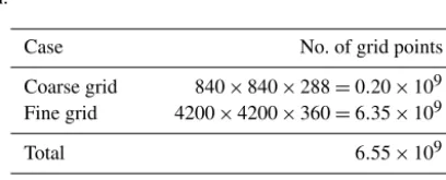
Table 4. Number of grid points in nested and non-nested FG do-main.
Case No. of grid points
Coarse grid 840×840×288=0.20×10⁹ Fine grid 4200×4200×360=6.35×10⁹
Total 6.55×10⁹
Non-nested FG 4200×4200×360=6.35×10⁹
by SA-C is only 8 core hours. While the nested simula-tions needed about 1879 core hours, the SA-F needed about 4 times more core hours than the nested simulation. As the resolution is increased from 20 m in SA-C to 4 m in SA-F, the number of time steps increased more than 5 times as higher resolution demands a smaller time step size. Though the number of time steps in FG is similar to SA-F, limiting the nested grid in the vertical direction has reduced the num-ber of CPU cores needed, and higher resolution in the surface layer is achieved at a reduced computational cost.
Several factors influence the computational performance of an LES code. Some factors depend on the hardware; e.g., the number of grid points per PE depends on the mem-ory available per node. On the other hand, the communi-cation time for data exchange between the PEs depends on the topology of the domain decomposition. The best perfor-mance in terms of communication time in a stand-alone run
Figure 4.Instantaneous contours of vertical velocity,(a)CG and(b)FG, at the verticalx−zcross section at the center of the domain after 10 800 s of the simulation. The dashed line in(a)marks the top of the overlapping region. Flow structures in the FG, which are similar but more detailed than the CG, qualitatively indicate the improvement to the surface layer resolution with the two-way nesting.
Figure 5. Vertical profile of horizontally averaged potential temperature normalized by the surface value(a, c)and variance of potential temperature normalized byθ∗2(b, d). The nested grid profiles agree well with the SA-F in the surface layer. The improvement of the two-way
Figure 6.Vertical profile of horizontally averaged heat flux normalized by the surface heat flux – resolved(a, d), sub-grid(b, e)and total flux(c, f). The two-way nesting significantly improves the resolved and SGS fluxes in the surface layer.
Table 5.Grid configuration of the nested and non-nested FG domain.
Nested Non-nested FG
Run Total CG FG Avg. time Efficiency Total Avg. time Efficiency PE PE PE per step (s) (%) PE per step (s) (%)
A 1664 64 1600 44.0 100 1600 14.9 100
B 3744 144 3600 19.9 98 3600 6.7 99
C 7488 288 7200 10.3 95 7200 3.6 92
D 8736 336 8400 9.3 90 8400 3.4 84
E 14 976 576 14 400 5.6 87 14 400 2.3 74
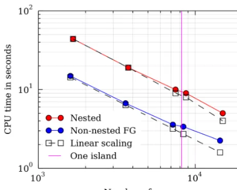
grid points, and such a large domain was computationally not feasible. The performance is measured in terms of the time taken to simulate one time step. To increase the accuracy of this performance measurement, the simulation is integrated for 10 time steps, and the average of the time per step is plotted. The results presented in Fig. 10 show close to linear scaling for up to 14 976 PEs in both nested and stand-alone runs. The difference in time per step between the nested and stand-alone runs can be interpreted as the additional compu-tational time needed by the nesting algorithm. A jump in the time taken to compute one step is observed when more than 8192 PEs are used. This is a hardware-dependent increase in communication time as the nodes are grouped as “islands” on SuperMUC system at the Leibniz Supercomputing Cen-tre. The communication within the nodes of the same island
is faster than the communication across multiple islands. The strong scaling efficiency in Table 4 is calculated, keeping the run with the lowest number of PEs as the reference. As the number of grid points per PE is reduced from run A to E as shown in Table 5, the nested runs show slightly better effi-ciency than the non-nested runs. The average time per step of the nested grid is 3 times higher than the non-nested setup for run A, but the factor decreases to about 2.5 for run E. This improvement is possibly due to reduction in waiting time be-tween the FG and CG as the number of grid points per PE decreases.
3.4 Practical considerations
Figure 7.Vertical profile of horizontally averaged resolved variance ofu(a, d),v(b, e), andw(c, f)normalized byw2∗. The variance ofv
andwshows better agreement with the stand-alone reference in the surface layer.
Figure 9.Spectra of SGS turbulent kinetic energy (e)(a, c)and vertical velocity (w)(b, d). Atz/zi=0.47(a, b)and atz/zi=0.11(c, d), kris the horizontal wavenumber.
select between Wicker–Skamarock (Wicker and Skamarock, 2002) and Piacsek–Williams (Piacsek and Williams, 1970) for the advection scheme. Similarly, for solving the Pois-son equation for the pressure, the user can choose between the FFT or multi-grid-based solver. During the develop-ment and the validation of the two-way nesting, only the Wicker–Skamarock advection scheme and FFT-based pres-sure solvers were tested. The two-way nesting supports only periodic boundary conditions in the horizontal for both CG and FG, and therefore an FFT-based pressure solver is an appropriate choice. However, to be able to use multi-grid solvers, e.g., in nonperiodic horizontal boundary con-ditions, modifications to the two-way nesting algorithm will be needed. The large-scale forcing feature in PALM is found to be compatible with the nesting algorithm without fur-ther modifications. Ofur-ther features like canopy parameteriza-tion, radiation models and land surface models have not been tested.
Our implementation of the vertical nesting allows only in-teger nesting ratios in all directions. The height of the nested
Figure 10. The nested simulations show close to linear scalabil-ity. A non-nested domain with same number of grid points as the FG is plotted to benchmark the scalability of the standard version of PALM on the same machine. The difference between the blue and the red line is approximately equal to the additional computa-tional time needed by the nesting routines. The simulations were performed on SuperMUC at the Leibniz Supercomputing Centre. Each node has 32 GB of main memory and two Sandy Bridge pro-cessors with 2.7 GHz; each processor has eight cores (Anastopoulos et al., 2013).
domain computationally feasible, care should be taken to en-sure the validity of such LES. In PALM, the height of the first grid point should be at the least twice greater than the local surface-roughness parameter. This technical restriction is common to all models that employ MOST and ensures the proper evaluation of the logarithm needed in the calculation ofu∗. Furthermore, Basu and Lacser (2017) recently recom-mended that MOST boundary conditions should be adapted for very high resolution LES, where the first grid point is smaller than 2–5 times the height of the roughness elements.
4 Summary
We presented a two-way grid nesting technique that enables high-resolution LES of the surface layer. In our concurrently parallel algorithm, the two grids with different resolution overlap in the region close to the surface. The grids are cou-pled, i.e the interpolation of the boundary conditions and the feedback to the parent grid are performed, at every sub-step of the Runge–Kutta time integration. The anterpolation of the TKE involves the Germano identity to ensure the conserva-tion of total kinetic energy. The exchange of data between the two grids is achieved by MPI communication routines, and the communication is optimized by derived data types. Re-sults of the convective boundary layer simulation show that grid nesting improves the vertical profiles of variance and the fluxes in the surface layer. In particular, the profiles of
the vertical temperature flux are improved. The current ver-tical nesting only works with periodic boundary conditions and with the same horizontal extent in both the domains. The nested simulation needs 4 times less computational time than a full high-resolution simulation for comparable accuracy in the surface layer. The scalability of the algorithm on up to 14 976 CPUs is demonstrated.
Code availability. The Parallelized Large-eddy simulation Model (PALM) is developed and maintained by the PALM group, Insti-tute of Meteorology and Climatology, Leibniz University Hannover (Raasch and Schröter, 2001; Maronga et al., 2015). The code is distributed under the GNU General Public License. The code (re-vision 2712) is available at https://palm.muk.uni-hannover.de/trac/ browser/palm?rev=2712 (last access: 24 June 2019).
Author contributions. SH was the main developer of the model code, with FDR as side developer, SR supporting the code devel-opment and MM, SR and FDR supervising the develdevel-opment. The experiment was designed by SH, FDR, SR and MM and carried out by SH, who also performed the validation. Visualization was done by SH and the original draft written by SH and FDR, with review and editing by SR and MM. MM was responsible for funding ac-quisition and administration.
Acknowledgements. This work was conducted within the Helmholtz Young Investigators Group “Capturing all relevant scales of biosphere-atmosphere exchange – the enigmatic energy balance closure problem”, which is funded by the Helmholtz Association through the President’s Initiative and Networking Fund and by KIT. Computer resources for this project have been provided by the Leibniz Supercomputing Centre under grant pr48la. We thank Gerald Steinfeld for sharing his original notes and code of a preliminary nesting method in PALM. We also thank Matthias Sühring and Farah Kanani-Sühring of the PALM group for their help in standardizing and porting the code, and we thank Michael Manhart for fruitful discussions.
Financial support. This research has been supported by the Helmholtz Association (grant no. VH-NG-843).
The article processing charges for this open-access publication were covered by a Research
Centre of the Helmholtz Association.
References
Anastopoulos, N., Nikunen, P., and Weinberg, V.: Best Practice Guide – SuperMUC v1.0. PRACE – Partnership for Advanced Computing in Europe 2013, available at: http://www.prace-ri.eu/ best-practice-guide-supermuc-html (last access: 24 June 2019), 2013.
Basu, S. and Lacser, A.: A Cautionary Note on the Use of Monin–Obukhov Similarity Theory in Very High-Resolution Large-Eddy Simulations, Bound.-Lay. Meteorol., 163, 351–355, https://doi.org/10.1007/s10546-016-0225-y, 2017.
Boersma, B. J., Kooper, M. N., Nieuwstadt, F. T. M., and Wessel-ing, P.: Local grid refinement in large-eddy simulations, J. Eng. Math., 32, 161–175, https://doi.org/10.1023/A:1004283921077, 1997.
Clark, T. L. and Farley, R. D.: Severe downslope windstorm cal-culations in two and three spatial dimensions using anelas-tic interactive grid nesting: A possible mechanism for gusti-ness, J. Atmos. Sci., 41, 329–350, https://doi.org/10.1175/1520-0469(1984)041<0329:SDWCIT>2.0.CO;2, 1984.
Clark, T. L. and Hall, W. D.: Multi-domain simulations of the time dependent Navier Stokes equation: Benchmark error anal-yses of nesting procedures, J. Comput. Phys., 92, 456–481, https://doi.org/10.1016/0021-9991(91)90218-A, 1991.
Daniels, M. H., Lundquist, K. A., Mirocha, J. D., Wiersema, D. J., and Chow, F. K.: A New Vertical Grid Nesting Capability in the Weather Research and Forecasting (WRF) Model, Mon. Weather Rev., 144, 3725–3747, https://doi.org/10.1175/mwr-d-16-0049.1, 2016.
Deardorff, J. W.: Three-dimensional numerical study of the height and the mean structure of a heated plane-tary boundary layer, Bound.-Lay. Meteorol., 7, 81–106, https://doi.org/10.1007/BF00224974, 1974.
Deardorff, J. W.: Stratocumulus-capped mixed layers derived from a three-dimensional model, Bound.-Lay. Meteorol., 18, 495–527, https://doi.org/10.1007/BF00119502, 1980.
Debreu, L., Marchesiello, P., Penven, P., and Cambon, L.: Two-way nesting in split-explicit ocean models: Algorithms, im-plementation and validation, Ocean Model., 49–50, 1–21, https://doi.org/10.1016/j.ocemod.2012.03.003, 2012.
Esau, I.: Indirect air–sea interactions simulated with a cou-pled turbulence-resolving model, Ocean Dynam., 64, 689–705, https://doi.org/10.1007/s10236-014-0712-y, 2014.
Flores, F., Garreaud, R., and Muñoz, R. C.: CFD simulations of turbulent buoyant atmospheric flows over complex geometry: Solver development in OpenFOAM, Comput. Fluids, 82, 1–13, https://doi.org/10.1016/j.compfluid.2013.04.029, 2013. Germano, M., Piomelli, U., Moin, P., and Cabot, W. H.: A dynamic
subgrid scale eddy viscosity model, Phys. Fluid A, 3, 1760–1765, https://doi.org/10.1063/1.857955, 1991.
Harris, L. M. and Durran, D. R.: An Idealized Comparison of One-Way and Two-One-Way Grid Nesting, Mon. Weather Rev., 138, 2174– 2187, https://doi.org/10.1175/2010mwr3080.1, 2010.
Kato, C., Kaiho, M., and Manabe, A.: An Overset Finite-Element Large-Eddy Simulation Method With Applications to Turbo-machinery and Aeroacoustics, J. Appl. Mech., 70, 32–43, https://doi.org/10.1115/1.1530637, 2003.
Khanna, S. and Brasseur, J. G.: Three-Dimensional Buoyancy- and Shear-Induced Local Structure of the Atmospheric Boundary Layer, J. Atmos.
Sci., 55, 710–743, https://doi.org/10.1175/1520-0469(1998)055<0710:tdbasi>2.0.co;2, 1998.
Kravchenko, A., Moin, P., and Moser, R.: Zonal Embed-ded Grids for Numerical Simulations of Wall-BounEmbed-ded Turbulent Flows, J. Comput. Phys., 127, 412–423, https://doi.org/10.1006/jcph.1996.0184, 1996.
Kröniger, K., De Roo, F., Brugger, P., Huq, S., Banerjee, T., Zinsser, J., Rotenberg, E., Yakir, D., Rohatyn, S., and Mauder, M.: Effect of Secondary Circulations on the Surface-Atmosphere Exchange of Energy at an Isolated Semi-arid Forest, Bound.-Lay. Meteo-rol., 169, 209–232, https://doi.org/10.1007/s10546-018-0370-6, 2018.
Kurihara, Y., Tripoli, G. J., and Bender, M. A.: Design of a Movable Nested-Mesh Primitive Equation Model, Mon. Weather Rev., 107, 239–249, https://doi.org/10.1175/1520-0493(1979)107<0239:doamnm>2.0.co;2, 1979.
Manhart, M.: A zonal grid algorithm for DNS of tur-bulent boundary layers, Comput. Fluids, 33, 435–461, https://doi.org/10.1016/S0045-7930(03)00061-6, 2004. Maronga, B., Gryschka, M., Heinze, R., Hoffmann, F.,
Kanani-Sühring, F., Keck, M., Ketelsen, K., Letzel, M. O., Kanani-Sühring, M., and Raasch, S.: The Parallelized Large-Eddy Simulation Model (PALM) version 4.0 for atmospheric and oceanic flows: model formulation, recent developments, and future perspectives, Geosci. Model Dev., 8, 2515–2551, https://doi.org/10.5194/gmd-8-2515-2015, 2015.
Moeng, C.-H. and Wyngaard, J. C.: Spectral analysis of large-eddy simulations of the convective boundary layer, J. Atmos. Sci., 45, 3573—3587, https://doi.org/10.1175/1520-0469(1988)045<3573:SAOLES>2.0.CO;2, 1988.
Moeng, C.-H., Dudhia, J., Klemp, J., and Sullivan, P.: Examining Two-Way Grid Nesting for Large Eddy Simulation of the PBL Using the WRF Model, Mon. Weather Rev., 135, 2295–2311, https://doi.org/10.1175/MWR3406.1, 2007.
Nakahashi, K., Togashi, F., and Sharov, D.: Intergrid-Boundary Def-inition Method for Overset Unstructured Grid Approach, AIAA J., 38, 2077–2084, https://doi.org/10.2514/2.869, 2000. Patton, E. G., Sullivan, P. P., Shaw, R. H., Finnigan, J. J., and Weil,
J. C.: Atmospheric Stability Influences on Coupled Boundary Layer and Canopy Turbulence, J. Atmos. Sci., 73, 1621–1647, https://doi.org/10.1175/jas-d-15-0068.1, 2016.
Piacsek, S. A. and Williams, G. P.: Conservation properties of con-vection difference schemes, J. Comput. Phys., 198, 500–616, https://doi.org/10.1016/0021-9991(70)90038-0, 1970.
Raasch, S. and Schröter, M.: PALM – A large-eddy simulation model performing on massively parallel computers, Meteorol. Z., 10, 363–372, https://doi.org/10.1127/0941-2948/2001/0010-0363, 2001.
Reynolds, W. C.: The potential and limitations of direct and large eddy simulations, in: Whither Turbulence? Turbulence at the Crossroads, edited by: Lumley, J. L., Springer Berlin Hei-delberg, Berlin, HeiHei-delberg, 313–343, https://doi.org/10.1007/3-540-52535-1_52, 1990.
Saiki, E. M., Moeng, C.-H., and Sullivan, P. P.: Large-eddy simula-tion of the stably stratified planetary boundary layer, Bound.-Lay. Meteorol., 95, 1–30, https://doi.org/10.1023/A:1002428223156, 2000.
large-eddy simulations, J. Fluid. Mech., 200, 511–562, https://doi.org/10.1017/S0022112089000753, 1989.
Skamarock, W., Klemp, J., Dudhia, J., Gill, D., Barker, D., Wang, W., Huang, X.-Y., and Duda, M.: A Description of the Advanced Research WRF Version 3, https://doi.org/10.5065/d68s4mvh, 2008.
Sullivan, P. P., McWilliams, J. C., and Moeng, C.-H.: A grid nesting method for large-eddy simulation of planetary boundary layer flows, Bound.-Lay. Meteorol., 80, 167–202, https://doi.org/10.1007/BF00119016, 1996.
van Hooft, J. A., Popinet, S., van Heerwaarden, C. C., van der Linden, S. J. A., de Roode, S. R., and van de Wiel, B. J. H.: Towards Adaptive Grids for Atmospheric Boundary-Layer Simulations, Bound.-Lay. Meteorol., 167, 421–443, https://doi.org/10.1007/s10546-018-0335-9, 2018.
Wang, G., Duchaine, F., Papadogiannis, D., Duran, I., Moreau, S., and Gicquel, L. Y.: An overset grid method for large eddy simu-lation of turbomachinery stages, J. Comput. Phys., 274, 333–355, https://doi.org/10.1016/j.jcp.2014.06.006, 2014.
Wicker, L. J. and Skamarock, W. C.: Time-splitting meth-ods for elastic models using forward time schemes, Mon. Weather Rev., 130, 2008–2097, https://doi.org/10.1175/1520-0493(2002)130<2088:TSMFEM>2.0.CO;2, 2002.
Williamson, J. H.: Low-storage Runge-Kutta schemes, J. Comput. Phys., 35, 48–56, https://doi.org/10.1016/0021-9991(80)90033-9, 1980.