https://doi.org/10.5194/gmd-12-69-2019
© Author(s) 2019. This work is distributed under the Creative Commons Attribution 4.0 License.
RandomFront 2.3: a physical parameterisation of fire spotting for
operational fire spread models – implementation in WRF-SFIRE
and response analysis with
LSFire+
Andrea Trucchia1,2, Vera Egorova1, Anton Butenko3,4, Inderpreet Kaur5, and Gianni Pagnini1,6
1BCAM–Basque Center for Applied Mathematics, Bilbao, Basque Country, Spain
2Department of Mathematics, University of the Basque Country UPV/EHU, Bilbao, Basque Country, Spain 3Space Research Institute of Russian Academy of Sciences, Moscow, Russia
4Institute of Geography, University of Bremen, Bremen, Germany
5Department of Atmospheric Chemistry, Max Planck Institute for Chemistry, Mainz, Germany 6Ikerbasque–Basque Foundation for Science, Bilbao, Basque Country, Spain
Correspondence:Gianni Pagnini ([email protected]) Received: 6 February 2018 – Discussion started: 19 March 2018
Revised: 17 October 2018 – Accepted: 28 November 2018 – Published: 3 January 2019
Abstract. Fire spotting is often responsible for dangerous flare-ups in wildfires and causes secondary ignitions isolated from the primary fire zone, which lead to perilous situations. The main aim of the present research is to provide a versa-tile probabilistic model for fire spotting that is suitable for implementation as a post-processing scheme at each time step in any of the existing operational large-scale wildfire propagation models, without calling for any major changes in the original framework. In particular, a complete physical parameterisation of fire spotting is presented and the corre-sponding updated model RandomFront 2.3 is implemented in a coupled fire–atmosphere model: WRF-SFIRE. A test case is simulated and discussed. Moreover, the results from dif-ferent simulations with a simple model based on the level set method, namelyLSFire+, highlight the response of the pa-rameterisation to varying fire intensities, wind conditions and different firebrand radii. The contribution of the firebrands to increasing the fire perimeter varies according to differ-ent concurrdiffer-ent conditions, and the simulations show results in agreement with the physical processes. Among the many rigorous approaches available in the literature to model fire-brand transport and distribution, the approach presented here proves to be simple yet versatile for application to opera-tional large-scale fire spread models.
1 Introduction
Fire spotting is an important phenomenon associated with wildfires (Fernandez-Pello, 2017). It is documented as a dominant aspect that has contributed to the rampant spread of fire in many devastating historical fires (Koo et al., 2010). Spot fires occur when fragments of the fuel tear off from the main fuel source and horizontal wind transports the burn-ing embers beyond the zone of direct ignition. The burnburn-ing embers/firebrands can develop new secondary ignition spots and lead to a perilous increase in the effective rate of spread (ROS) of the fire.
The main aim of the present research is to provide a versa-tile probabilistic model for fire spotting that is suitable for implementation as a post-processing scheme at each time step in any of the existing large-scale operational codes for simulating wildfire propagation, without calling for any ma-jor changes in the original framework.
(Manzello et al., 2008). The short temporal and spatial scales of the experiments limit a detailed description of the landing distributions and flight paths of the firebrands. Conversely, firebrand transport models provide an estimate of the maxi-mum landing distance and flight paths of firebrands through a simplified overview of the physical dynamics of fire be-haviour, plume characteristics and the atmospheric condi-tions around the fire. Tarifa et al. (1965, 1967) and Albini (1979, 1983) were the first to develop simplified plume mod-els for the estimation of firebrand lifetimes, flight paths and potential fire-spotting distance. Beginning with their stud-ies, there has been a paradigm shift in the development of firebrand transport models, with the latest models benefiting from advanced computational techniques and resources.
Woycheese et al. (1999) provide a model for the lofting of spherical and cylindrical firebrands using the plume model proposed by Baum and McCaffrey (1989). They suggest an-alytical functions for the maximum loftable diameter and the maximum loftable height in terms of the fire intensity, atmo-spheric wind and the fuel characteristics. Numerical experi-ments by Sardoy and co-workers (Sardoy et al., 2007, 2008) also analyse the effect of atmospheric conditions, fire prop-erties and fuel propprop-erties on firebrand behaviour and pro-vide a statistical estimate of the ground level distributions of disk shaped firebrands. Their results highlight that fire-brands landing at short distances (up to 1000 m) from the source follow a lognormal distribution. A study by Wang (2011) also provides a mathematical model to quantify the distribution and the mass of firebrands through a Rayleigh distribution function. In an another study, Koo et al. (2007) present a physics based multiphase transport model for wild-fires (FIRETEC) to study firebrand transport. In a recent study, Martin and Hillen (2016) also discuss the underlying physical processes for firebrands in detail and derive a land-ing distribution based on these physical processes. Besides these statistical approaches, a few numerical models based on large eddy simulation (LES) (Himoto and Tanaka, 2005; Pereira et al., 2015; Thurston et al., 2017; Tohidi and Kaye, 2017) or computational fluid dynamics (CFD) (Wadhwani et al., 2017), small world networks (Porterie et al., 2007) and cellular automata models (Perryman et al., 2013) also exist in the literature. Bhutia et al. (2010) present one such study based on a coupled fire–atmosphere LES for predicting short-range fire spotting. They simulate multiple firebrand trajecto-ries for analysing the sensitivity of the flight path to different particle sizes, release heights and wind conditions but also mention the limited applicability of such models to opera-tional use due to the computaopera-tional demands.
Despite the presence of multiple studies focusing on the detailed aspects of firebrand landing distributions, none of them are able to provide a comprehensive yet versatile ap-proach for an application to operational fire spread models. The continuing demand for operational management tools is to provide a quick and efficient output with simple in-puts but at the same time to take the most important
pa-rameters into consideration. A few operational fire spread models like FARSITE (Finney, 1998), BEHAVEPLUS (An-drews and Chase, 1989) and Prometheus (Tymstra et al., 2010) incorporate the phenomenon of fire spotting through the Albini’s model (Albini, 1979, 1983). However, the Al-bini’s model only provides an estimate of the maximum dis-tance for a spot fire and does not include any function for the ignition probability to model the spread of spot fires. The Australian wildfire simulator PHOENIX RapidFire (Tolhurst et al., 2008) is designed to model large fast moving fires and also includes a fire-spotting module; however, the formula-tions for fire spread in PHOENIX are calibrated for eucalyp-tus forests and a generic application to other types of fuels requires a recalibration (Pugnet et al., 2013). The new oper-ational models like WRF-SFIRE (Mandel et al., 2011) and FOREFIRE (Filippi et al., 2009) are fast and allow coupling with atmospheric models for a better representation of the initial and concurrent atmospheric conditions; but they lack any specific module to tackle fire-spotting behaviour.
In this article, the authors proceed with the RandomFront statistical formulation for including the effects of random processes in wildfire simulators, namely turbulence and fire-spotting phenomena. The chronology of this approach refers to the following papers: v1.0 includes only turbulence, with no parameterisation (Pagnini and Massidda, 2012a, b); v2.0 includes turbulence and fire spotting with literature param-eterisation for fire spotting (Pagnini and Mentrelli, 2014); v2.1 includes turbulence and fire spotting with parameteri-sation for turbulence (Kaur et al., 2016); and v2.2 includes turbulence and fire spotting with a first physical parameter-isation of fire spotting (Kaur and Pagnini, 2016). Finally, in the present version v2.3 the parameterisation of fire spotting has been modified and corrected (also in view of a remark by one of the referees) with respect to the previous version.
et al., 2014) and a paradigmatic test case has been simu-lated. Moreover, the proposed formulation for including ran-dom process and the corresponding physical parameterisa-tions are implemented into a much simpler fire spread sim-ulator, also based on the LSM, namely LSFire+(Pagnini and Massidda, 2012a, b; Pagnini and Mentrelli, 2014; Chu and Prodanovi´c, 2009; Bevins, 1996). Results from differ-ent test cases withLSFire+are presented to highlight the sensitivity of the simple parameterisation in simulating the generation of secondary fires by fire spotting under different wind conditions, fire intensities and firebrand radii.
The article is organised as follows. In Sect. 2 a very brief description of the mathematical model is presented, while the physical parameterisation of fire spotting within the frame-work of a lognormal distribution of the landing distance is described in Sect. 3. The implementation of RandomFront 2.3 in the computational environments WRF-SFIRE in addi-tion to a test case and the corresponding discussion are re-ported in Sect. 4, and the implementation inLSFire+and the corresponding response analysis are discussed in Sect. 5. Conclusions are drawn in Sect. 6.
2 Model formulation
A mathematical model to represent the random effects asso-ciated with the wildland fires has been developed by Pagnini and co-authors (Pagnini and Massidda, 2012b, a; Pagnini, 2013, 2014; Pagnini and Mentrelli, 2016, 2014; Kaur et al., 2015, 2016; Mentrelli and Pagnini, 2016). This formulation describes the motion of the fire line as a composition of the drifting part and the fluctuating part. The drifting part represents the fire perimeter obtained through the definition of the ROS based on fuel characteristics and the averaged fire properties. The output from most of the existing oper-ational fire spread models can be considered as the drifting part. Conversely, the fluctuating part is independent of the drifting part and represents the additional contribution to the fire perimeter as an effect of random processes like turbu-lence and fire spotting. This model can be implemented as a crucial addition to operational fire spread models through a post-processing application at each time step. The drifting component obtained from the output of any wildfire model can be updated with the fluctuating component at each time step to include the effects of turbulence and fire spotting. A brief overview of the mathematical details is provided in the following; for a detailed description readers are referred to Pagnini and Mentrelli (2014) and Kaur et al. (2016).
In a domainS, let⊆Srepresent the burnt area and let Xω=X+ηωrepresent the trajectory of each active fire point as the sum of a drifting part X and a fluctuating part ηω. The drifting partXis obtained from the output of a wildfire propagation model, while the fluctuations in the fire-line are included through a probability density function (PDF) cor-responding to the type of random process under
considera-tion. Let the area enclosed by the drifting part be described through an indicator functionI(x, t )=1 whenx is inside the domain, andI(x, t )=0 whenxis outside. Consider-ing the ensemble average of the active burnConsider-ing points, a new effective indicator function is defined as follows:
φe(x, t )=
Z
S
I(x, t )f (x;t|x)dx, (1)
wheref (x;t|x)represents the PDF which accounts for the fluctuations of the random effects. The effective indicator φe∈ [0,1], and an arbitrary threshold is fixed to mark points
as burned, i.e.e(x, t )= {x∈S|φe(x, t ) > φeth}. The
igni-tion of fuel by firebrands involves heat exchange over a suffi-cient period of time; therefore, a suffisuffi-cient delay is also incor-porated in the model through another function:ψ. The func-tionψsimulates the ignition of fuel by hot air and burning embers as an accumulative process over time (the heating-before-burning mechanism):
ψ (x, t )= t Z
0
φe(x, η)
dη
τ , (2)
whereτ is the ignition delay. At each timet, all pointsx that satisfy the conditionsψ (x, t ) >1 orφe(x, t ) > φthe are
labelled as burned.
The shape of the PDFf (x;t|x)is established by analysing the random processes under consideration. The diversity in the shapes of the PDF provides the model a multifaceted out-look. Assuming fire spotting to be a downwind phenomenon occurring in turbulent atmosphere, the shape of the PDF is defined as follows:
f (x;t|x)=
Z ∞
0
G(x−x−lnˆU;t )q(l)dl, downwind,
G(x−x;t ), upwind.
and Tanaka, 2005; Kortas et al., 2009). Among the differ-ent transport models proposed in the literature, both Sardoy et al. (2008) and Himoto and Tanaka (2005) describe the log-normal density function as an approximate fit to the landing distribution of firebrands. Wang (2011), in comparison, pro-poses a Rayleigh distribution for the same. In this article, the shape of q(l)is defined by a lognormal distribution to de-scribe the frequency profile of the fallen firebrands:
q(l)=√ 1 2π σ lexp
−(lnl/µ)2
2σ2 , (4)
whereµis the ratio between the square of the mean of the landing distancel and its standard deviation, whileσ is the standard deviation of lnl/µ.
3 Physical parameterisation of fire spotting
The firebrands generated from vegetation face strong buoy-ant forces and those with a size less than the maximum loftable size are vertically uplifted in the convective column. These firebrands rise to a maximum height until the buoy-ant and the gravitational forces counterbalance one another. Once the firebrands are expelled from the column, they are steered by atmospheric wind and fly at their terminal veloc-ity of fall. Simplified models for the landing distance assume that the ejection of firebrands from the vertical convective column is a random process affected by the turbulence in the environment around the fire. Among other factors, the strength of the convective column, the atmospheric condi-tions and the dimensions of firebrands play a vital role in governing the trajectory of the firebrands. In this section, the landing distribution of firebrands based on a lognormal prob-ability function is combined with the physical characterisa-tion of firebrand transport. The parameterisacharacterisa-tion presented here is simplified and only includes the vital ingredients nec-essary to describe firebrand transport. Each firebrand is as-sumed to be spherical and for a particular set of concurrent atmospheric conditions and fuel characteristics, and the size is assumed to be constant. Any modification in the flight of the firebrand due to rotation of the firebrand or collision with other firebrands is also neglected. Preliminary results were discussed in Kaur and Pagnini (2016).
Literature studies identify the maximum spotting distance as a numerical measure to assess the severity of the fire-spotting danger under different circumstances (Albini, 1979; Tarifa et al., 1965, 1967). Recognising the importance of maximum-spotting distance, we select to parameterise the mathematical model in terms of thepth percentile of a log-normal distribution as a measure of the maximum landing distance. The pth percentile for a lognormal distribution is described by its location and shape parametersµandσ, re-spectively:
L=µexp(zpσ ) , (5)
where the value ofzpcorresponding to thepth percentile can be estimated from theZ-table (see, for example, http://www. itl.nist.gov/div898/handbook/eda/section3/eda3671.htm, last access: 19 December 2018). We hypothesise that the pth percentile represents the maximum landing distance for fire-brands under different situations and that no ignition is pos-sible beyond this cut-off. To ascertain the value of the “cut-off” percentile, it is assumed that the effective contribution of the firebrands ceases to be meaningful when its probabil-ity reduces to 20 times its peak value. Thereafter, the abilprobabil-ity of the firebrands to cause an ignition is assumed to be neg-ligible. The cut-off criteria is chosen empirically, but a suf-ficiently large number (like 20) ensures that we do not miss any considerable fire-spotting behaviour that exists outside this range.
For this particular distribution, the cut-off for the 50th per-centile lies way beyond the point denoting 1/20th of the max-imum probability. In order to define a generalized value of the cut-off percentile for all of the simulation cases presented in this paper, the value ofzpis set to 0.45, which corresponds to the 67th percentile point.
The process of fire spotting can be roughly segregated into generation, lofting and transport of firebrands. The genera-tion of firebrands from a burning canopy is a random and dy-namic process, while the lofting and transport of firebrands is regulated by the firebrand geometry, fuel combustion rates, plume dynamics and ambient wind conditions. The different sub-processes involved in firebrand lofting and transport in-teract with each other and affect the maximum spotting dis-tances. An explicit modelling of the coupled processes is dif-ficult and different approximations and assumptions are of-ten used to simplify the physical processes. An example of important works on fire-spotting distributions and maximum spotting distances are those by Tarifa and co-workers (Tar-ifa et al., 1965, 1967). In their different publications they describe spotting distributions and maximum spotting dis-tances by combining a series of experimental and theoretical approaches. We follow these existing approaches and formu-late the physical parameterization for our model. Below we provide a brief discussion of the different processes which are considered in the physical parameterization:
1. Firebrand lofting
(a) Vertical gas flow: in a convective column, the up-draught introduced by the fire lifts the firebrands in the convective column. The strength of vertical gas flowUgas increases with the fire intensityI and is
empirically expressed as in Muraszew (1974):
Ugas=9.35
I
Hc
1/3
, (6)
whereHcis the heat of combustion of wildland
(b) Size of firebrands: the convective activity inside the plume regulates the maximum size of the firebrand that can be lofted. The terminal velocities of the loftable firebrands can not exceed the vertical gas flow rate. As the vertical gas-flow increases with increasing fire rate, heavier firebrands can be up-lifted into the plume. In the literature, the maximum loftable radius for spherical firebrands is expressed as follows (Tarifa et al., 1965; Albini, 1979; Wang, 2011):
rmax=
3 2Cd
ρa
ρf
Ugas2
g , (7)
whereρaandρfrepresent the density of the ambient
air and wild-land fuels, respectively,Cdis the drag
coefficient andgis the acceleration due to gravity. (c) Maximum loftable height: Wang (2011) and
Woy-cheese et al. (1999) parameterise the maximum loftable height for spherical firebrands in terms of the radius of firebrandr, constrained by the maxi-mum radius of the firebrandsrmax:
H=1.46 ρ
f
ρaCd
r5/2
max
r3/2. (8)
2. Horizontal transport:
(a) Maximum landing distance: assuming the shape of the firebrands to be spherical, the study by Tarifa et al. (1965) combines both experimental and the-oretical approaches to characterise the maximum landing distances of firebrands. Based on these re-sults, Wang (2011) provides an approximation of the maximum travel distance for spherical fire-brands from a vertical convective column in terms of the following: maximum loftable heightH; the meteorological mean windU = |Uh|, whereUhis
the horizontal wind vector field at fire height; and the radius of the firebrandsr. This results in the fol-lowing equation:
L=H U Ugas
rmax r
1/2
. (9)
3. Ignition probability: as described in the previous sec-tion, the probability that fuel is ignited by burning em-bers is modelled using the functionψ(Eq. 2). Here we assume that the fuel conditions are homogeneous and the ignition probability only depends on an ignition de-layτ. No other local variables are taken into account. 4. Secondary fire-lines: the secondary emissions
gener-ated during fire-spotting modelling are assumed as new sources of fire with a proper fire intensity. These new fires act as additional input along with the primary fire
towards the generation of other secondary fires; it is as-sumed that these new sources are capable of generating firebrands of the same size as the primary source. Small-scale processes, such as the mass loss of a firebrand due to combustion, affect the fire-spotting phenomenon by generating random fluctuations in the firebrand trajectory. These fluctuations are embodied by the use of a distribution for the landing distance.
Finally, the above large-scale sub-processes under lofting and transport mechanisms are linked through Eq. (5) to ob-tain the physical parameterisation ofµandσ of the lognor-mal distribution. Using Eqs. (9) and (8), we express the shape and location parameters as follows:
σ= 1 2zp ln U2 rg , (10)
µ=H 3
2 ρa
ρf
Cd
1/2
. (11)
We chose such a parameterization of µ and σ in order to delineate the governing parameters for lofting and trans-port mechanisms, respectively. We hypothesise that the def-inition ofµcovers the essential input parameters needed to describe the lofting mechanism of firebrands inside the con-vective column. The relative densityρa/ρfand atmospheric
drag quantify the buoyant forces experienced by the fire-brand; hence, it is appropriate to include these quantities in the definition of µ. Substituting maximum loftable height from Eq. (8) inµgives
µ=3.52×10⁵ ρ
a
ρf
Cd
2 I Hc
5/3
r−3/2g−5/2. (12) The radius of the firebrandrand the fuel density are impor-tant factors regarding the determination of the height of the lofted firebrands. Conversely,σis hypothesised to define the transport of firebrands under the effect of horizontal wind af-ter ejection from the convective column. The definition ofσ includes a dimensionless ratioF=U2/(rg) which is
anal-ogous to the Froude number, which quantifies the balance between inertial and gravitational forces experienced by fire-brands. All firebrands withr≤U2/gcan be transported by
horizontal wind.
Table 1.List of the symbols used to describe the model quantities and the parameters used in this study.
Model quantities Units
φe Effective indicator –
ψ Ignition function –
x=(x, y) Horizontal space variable m
t Time s
f Probability density function of the random processes m−2 G(x;t )) Isotropic bivariate Gaussian probability density m−2 q(l) Lognormal distribution of firebrand landing m−1
Parameters
Static parameters Value
µ Parameter ofq(l) –
σ Parameter ofq(l) –
D Turbulent diffusion coefficient ofG 0.15 m2s−1
ρa Density of air 1.2 kg m−3
ρf Density of wildland fuel (Pinus ponderosa) 542 kg m−3
Cd Drag coefficient 0.45
zp pth percentile 0.45
g Acceleration due to gravity 9.8 m s−1 Hc Heat of combustion of wildland fuels 18 620 kJ kg−1
ω0 Oven-dry mass of fuel 2.243 kg m−2
H Fuel low heat of combustion 22 000 kJ kg−1
Dynamic parameters Units
U=(U, V , W ) Wind vector at fire height m s−1 Uh=(U, V ) Horizontal wind vector field at fire height m s−1 τ Ignition delay of firebrands s
I Fire-line intensity MW m−1
Ugas Vertical gas flow m s−1
r Radius of spherical firebrand m rmax Maximum loftable radius for spherical firebrand m
H Maximum loftable height for spherical firebrands m
Vros Rate of spread m s−1
that the Nusselt number is related to the Rayleigh num-ber asNu'0.1Ra1/3(Niemela and Sreenivasan, 2006). The Rayleigh number is defined asRa=γ 1T gh3/(νχ ), where γ =3.4×10⁻³K−1is the thermal expansion coefficient,his
the dimension of the convective cell,ν=1.5×10⁻⁵m2s−1 is the kinematic viscosity and1T is the temperature gradi-ent between the top and bottom faces of the convective cell. Finally, we estimate the turbulent diffusion coefficient using the following formula:
D'0.1 γ g
ν 1/3
χ2/31T1/3h−χ , (13) and assuming 1T '1000 K andh'100 m, we have D∼ 10−1m2s−1. For all of the simulations presented in this ar-ticle, the value of the turbulent diffusion coefficientDis as-sumed to be 0.15 m2s−1.
The simple design of the physical parameterisation makes the model computationally less expensive, and the
require-Table 2.Values of the main parameters for numerical simulations performed withLSFire+.
Unit of First Second Quantity measurement test case test case
D m s−1 0.15 0.15 U m s−1 10 2/26 I MW m−1 5/100 50 r m 0.015 0.015/0.03
τ s 1 1
4 Numerical simulations
The detailed steps of the numerical procedure are as follows (Kaur et al., 2016):
1. Beginning with an initial fire line, an operational code, i.e. WRF-SFIRE in this section and LSFire+in the next section, is used to estimate the propagation of the front and to generate a new fire perimeter for the next time step. This output is modified to include the effects of turbulence and fire spotting using a “post-processing numerical procedure”. This post-processing step is in-dependent of the definition of the ROS.
2. The fire perimeter obtained from the chosen operational code is used to construct the indicator functionI(x, t ), i.e. the indicator functionI(x, t )has a value of 1 in-side the domain surrounded by the fire-line and 0 out-side of the domain. The spatial information contained in I(x, t )is necessary to modify the fire line with respect to turbulence and fire spotting and serves as an input to the post-processing step.
3. The effective indicator functionφe(x, t )(Eq. 1) is
gen-erated over a Cartesian grid to facilitate the computation of the functionψ (x, t )(Eq. 2) over the same grid. 4. The value of the effective indicatorφe(x, t )is computed
through the numerical integration of the product of the indicator functionI(x, t )and the PDF of fluctuations according to Eq. (1). The effect of turbulence or fire spotting is included by choosing the corresponding PDF (Eq. 3).
5. The functionψ (x, t )is updated for each grid point by integration in time with the current value ofφe(x, t ).
6. All points that satisfy the conditionψ (x, t )≥1 are la-belled as new ignition spots. The post-processing pro-cedure is completed at this step.
7. At the next time step, the new fire perimeter evolves ac-cording to the chosen operational code, and the updated perimeter is again subjected to the post-processing pro-cedure to enrich the fire front with the random fluctua-tions pertaining to turbulence and fire spotting. The se-quence is repeated until the final “event time” step or until the fire reaches the boundaries of the domain. 4.1 Implementation of RandomFront 2.3 in
WRF-SFIRE
In order to prove the viability of the proposed formulation within an operational code, we implemented RandomFront 2.3 in the framework of the WRF-SFIRE simulator (Coen et al., 2012; Mandel et al., 2014). WRF-SFIRE is a cou-pled fire–atmosphere model, which operates in the compu-tational environment of a well-known public domain numer-ical weather prediction model: WRF v3.4 (Weather Research
and Forecasting; Skamarock et al., 2008; https://www.mmm. ucar.edu/weather-research-and-forecasting-model, last ac-cess: 19 December 2018).
The fire module embedded into WRF simulates a sur-face fire and takes a two-way coupling with the atmospheric model into account. The near-surface winds from the atmo-spheric model are interpolated on the fire grid and are used along with fuel properties and local terrain gradients to com-pute both the ROS and the outward front-direction, which are further used as an input to the front propagation routines through a LSM scheme. Fuel consumption is responsible for the release of sensible and latent heat into the lowest lay-ers of the atmosphere, and this has a role in the computation of the boundary-layer meteorology. Recently, the model has been equipped with a fuel-moisture sub-model and a chem-istry sub-model (WRF Chem), which contribute to reproduc-ing and investigatreproduc-ing the effects of the fire–atmosphere cou-pling.
Coen et al. (2012) points out that fires generally start from a horizontal extent much smaller than the size of the fire mesh-cell. The same may be argued for the secondary ig-nitions related to fire-spotting phenomenon. In this respect, Coen et al. (2012) propose (and explain in detail) an al-gorithm for a punctual or line ignition that actually runs on WRF-SFIRE. The purpose of this algorithm is two-fold: (i) it guarantees from a physical point of view that the igni-tion starts at sub-grid scale without generating unrealistically large initial heat flux and an accelerated ignition; (ii) this pro-cedure is numerically robust because it is fully integrated into the representation in terms of a “signed distance function” of the LSM (Sethian and Smereka, 2003).
In the proposed formulation, a punctual ignition occurs whenever the conditionψ (x, t )≥1 holds true. This proce-dure is not computationally viable so we set a threshold dis-tanceRth=200 m for separating each pair of punctual
igni-tions. In particular, letPbe the set of point-wise fire-spotting ignitions, the actual algorithm performed at each time step within WRF-SFIRE model is reported in Algorithm 1.
4.2 Discussion of the test case with WRF-SFIRE
In this paper we consider a slight modification of thehill
test case (https://github.com/openwfm/wrf-fire/blob/master/ wrfv2_fire/test/em_fire/hill/namelist.input.hill, last access: 19 December 2018). In order to simplify the underlying dy-namics, but maintain the fire–atmosphere coupling, the hill is suppressed (fire_mountain_type = 0) and we have a square-grid simulation over a flat domain with a side length of 2.5 km. The horizontal atmospheric grid-spacing at terrain-height is 60 m, while the fire spread grid-spacing is 15 m. The simulation starts at t=0 min and ends at t=20 min. The fire line is initially located along the segment joining the points (1900 m, 1500 m) and (1900 m, 1800 m), and the initial wind field at the fire height is (U (x;t=0),V (x;t= 0))=(−6.4 m s−1,−3.6 m s−1) at all points in the simulation domain.
The fuel has been set equal to fire “Type 9”, i.e. “FM 9 hardwood litter” according to Anderson classification (An-derson, 1982). This fuel type may represent a terrain cov-ered byP. ponderosa trees. The radius of spherical embers was set equal tor=12.5 mm following a size considered by Manzello et al. (2006) with respect to the same vegetation.
Concerning the proposed formulation, the fire-line inten-sityIand the wind field are computed using the WRF-SFIRE model; this allows for a varying field of both parametersσ andµaccording to Eqs. (10) and (12), respectively. In partic-ular, following the latest advancements of the SFIRE model environment in Mandel et al. (2014), the spatial represen-tation of the potential-fire characteristics are available from which a field extension of the fire-line intensity I is avail-able in order to have a space and time varying field of µ for the fire-spotting routines. ParametersDandτ are set as
D=0.15 m2s−1andτ =8 s, without using estimations from WRF-SFIRE.
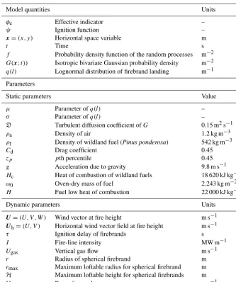
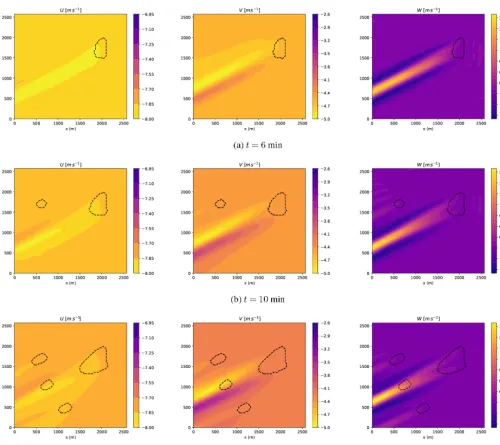
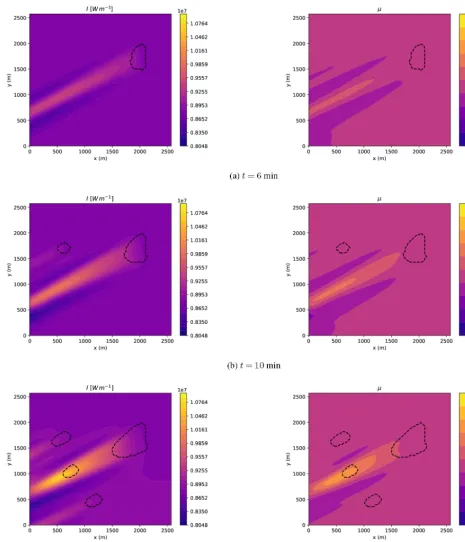
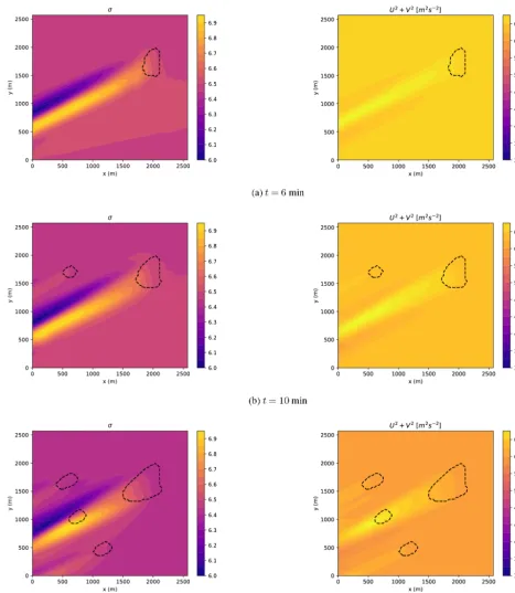
Figures 1–3 display the simulation results. In each figure the fire front is represented by a dashed line at the following instantst=6 min,t=10 min and t=20 min. The selected instants allow for the observation of the propagation of the main fire alone, the generation of a secondary fire and the multi-generation of secondary fires. In particular, in Fig. 1 the evolution of the fire line is shown in relation to the three components of the wind field; Fig. 2 shows the relationship with the parameterµand the fire intensity field; Fig. 3 shows the relationship with the parameterσ and the squared norm of the horizontal wind.
Overall, we observe that the fire-line propagation is “pulled” in the direction of the maximum value of the squared norm of the horizontal wind (see right column in Fig. 3); this direction is induced by the fire itself as a feed-back on the weather as is shown by the patterns of the at-mospheric observables when secondary fires are generated. The geometrical profile of the fire perimeter always plays an important role in determining fire-spotting behaviour. The asymmetry in the fire perimeter at 20 min along the
promi-nent direction of propagation, causes the first secondary fire to appear in the top-left part of the domain. With time, as the fire-activity increases, the differences between the max-imum value of the squared norm of the horizontal wind and its surroundings increase and the fire-line becomes symmet-rical with respect to the main direction of propagation. This has a direct influence on the fire-spotting action, and the new secondary fires appear increasingly aligned towards the main direction of propagation.
The secondary fires are equally as important as the pri-mary fire with respect to influencing the weather around the fire. The plots clearly show the influence of fire–atmosphere coupling, and feedback dynamics from secondary fires to pri-mary fire can be also observed. The secondary fires affect the wind (see Fig. 1) and the parameterσ (Fig. 3), which im-plies a refinement in fire-spotting characteristics for further ignitions. A point worth noting is that the first secondary fire occurs at a distance of almost 1500 m from the main fire. This observation supports the viability of the proposed for-mulation to simulate the fire-spotting mechanism in stud-ies of large-scale fires. However, if the implementation in WRF-SFIRE allows for a comprehensive picture including the physical features of a multi-scale and multi-physics pro-cess, the complexity of the model, the number of parameters and the numerical cost increases.
In the next section, we perform a response analysis of our parameterisation, by using the simple finite difference code
LSFire+, which allows for extensive simulations in terms of the spatial domain and simulation time. A sensitivity anal-ysis on the inputs and an uncertainty quantification on the outputs of RandomFront implemented inLSFire+will be considered in a separate paper.
5 Response analysis
5.1 Implementation of RandomFront 2.3 inLSFire+
A few idealised simulations are carried out to highlight the potential applicability of the formulation. For all the simu-lations, a flat domain with a homogeneous coverage of aP. ponderosaecosystem is selected, as seen in the WRF-SFIRE implementation. The simulations are run using a basic set-up of the wildfire modelLSFire+which involves a moving interface method based on the LSM (Pagnini and Massidda, 2012a, b; Pagnini and Mentrelli, 2014). The Byram formula (Byram, 1959; Alexander, 1982) is used to estimate the ROS of the fire line:
Vros(x, t )=
I (1+fw)
H αω0
, (14)
whereI is the fire intensity,H=22 000 kJ kg−1is the fuel low heat of combustion,ω0=2.243 kg m−2is the oven-dry
Figure 1.Wind vector components (U,V W) performed with WRF-SFIRE at timest=6, 10 and 20 min. The fire front is represented by a dashed line.
introduce a different ecosystem into the simulations by mod-ifying the parametersH andω0. The parameterαis chosen
to guarantee that the maximum ROS is always equal to the ROS prescribed by the Byram formulation.
The response of the formulation with respect to depict-ing the different firebrand landdepict-ing distributions is highlighted through two sets of test cases. In the first test case, the wind conditions and the size of the firebrands are assumed to be constant as the fire intensity changes. In the second test case, the fire intensity is assumed to be constant and the simula-tions for different wind condisimula-tions are carried out. The sec-ond test case is also repeated for different firebrand radii.
For speeding-up all simulations presented in this section, the domain has been scaled by a factor of 4 to reduce the computation time. In the scaled mode each grid cell repre-sents 4×4 times the area of each grid cell of the original domain. This scaling also affects the ROS and the turbulent diffusion coefficient: their value is reduced by a factor of 4. Fire intensity and the wind speed remain unaffected by the rescaling. It is noted that such scaling has no effect on the outputs of the simulations but helps to reduce the computa-tion time.
Figure 2.Fire intensityIand PDF shape parameterµperformed with WRF-SFIRE at timest=6, 10 and 20 min. The fire front is represented by a dashed line.
all shapes and sizes of firebrands are produced from the fuel. It is also emphasized that the selection of the domain and other parameters do not correspond to any real fire, but an effort is made to chose values of the different parameters that lie within a valid range (Table 2).
5.2 Discussion of the test cases withLSFire+
formu-Figure 3.The PDF shape parameterσ and horizontal wind squared magnitude (|Uh|2) performed with WRF-SFIRE at timest=6, 10 and 20 min. The fire front is represented by a dashed line.
lation is its ability to incorporate the generation of secondary fires. Figure 4a–b show the evolution of the fire perimeter under the effect of turbulence and fire spotting. Figure 4a shows the effect of fire spotting in the presence of a barrier. This barrier is a fuel free zone with zero probability of
Figure 4. (a)Line contours showing the fire perimeter at different time steps with the presence of a fire barrier. The wind velocity is 10 m s−1, the fire intensity is 25 MW m−1and the diffusion coefficient is 0.15 m2s−1. Thexandyaxes of the plot are scaled by a factor of 4. The same plot is proposed in(b), but withU=20 m s−1and no barrier.(c)A comparison of the total burned area at different time steps when only turbulence is considered (black) and when both turbulence and fire spotting are included (red). The total burned area is simply the number of burned grid points at any each instant. For both line plots, the wind velocity is 10 m s−1, the fire intensity is 25 MW m−1and the diffusion coefficient is 0.15 m2s−1.
in the head and cross wind directions, but the secondary fires increase quickly under the effect of wind. The wavy pattern of the fire perimeter results from the merging of multiple secondary fires in an idealised set-up of constant conditions. Figure 4b shows the scenario where secondary fires appear without the presence of a barrier. The effect of firebrands first appears around 130 min, and the new secondary fire behaves as a separate fire and evolves accordingly. InLSFire+the effects of fire spotting occur in conjunction with turbulence, and both processes contribute towards the fire propagation. It is difficult to separate the effects of both processes indi-vidually, but a comparison of the increase in burned area due to turbulence and turbulence + fire spotting is presented in Fig. 4c. The total number of burned points is plotted at dif-ferent times for two simulations: only turbulence, and tur-bulence+fire spotting. All of the simulation parameters
re-main the same in both of the simulations. As the fire starts evolving, the line plots for both of the simulations overlap signifying that fire spotting has no visible contribution, but after 50 min the fire-spotting effect picks up and the burned area rapidly increases. At 140 min the increase in the burned area under the combined effect of the two random processes is almost three times the effect of turbulence alone.
For the response analysis, a separate set of simulations are carried out, and the response is evaluated using the parameter βe, which describes the effective increase in the burned area
as follows:
βe=(xrandom−xno-random)/xno-random. (15)
βeis simply the increase in the number of burned grid points
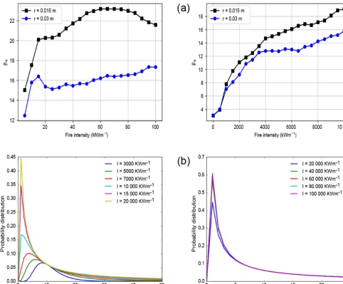
Figure 5. (a)Line plot showing the sensitivity of the formulation to different values of fire intensity over constant wind conditions (10 m s−1) and a constant firebrand radius (0.015 m). The sensitivity is measured in terms of the total increase in the burned area when both fire spotting and turbulence are included over the case when no random effects are considered. The parameterβeis defined asβe=(xrandom−
xno-random)/xno-random. The diffusion coefficientDis 0.15 m2s−1.(b)The line plots show the lognormal distribution for selected values of fire intensityIbut constant values of wind speedU=10 m s−1and firebrand radiusr=0.03 m. According to the physical parameterisation, the plots can also be interpreted as the behaviour of the lognormal distribution for varying values of the parameterµand a constant value of the parameterσ.
The simulated domain for the response analysis is cho-sen as a rectangle with the following dimensions (0 m, 6000 m )×(0 m, 6000 m). The simulations start at timet= 0 min and end at timet=140 min. The grid spacing is1x= 1y=20 m. At timet=0 min the initial fire line is a circle with a radius of 180 m centred atxc=(720 m, 3000 m). The horizontal wind is assumed as a constant field parallel to the vector j=(1,0)and with modulus|Uh| = |(U, V )| in this
simulation set-up.
Response analysis to fire intensity
An increase in the fire intensity causes an increase in the burned area (see Eq. 14 for the definition of the ROS); si-multaneously, the fire-spotting behaviour is also affected by any change inI. The parameterβeallows us to identify the
parameterisa-tion of the lognormal shape parametersµandσ, for this set of simulations (increase in fire intensityI), the parameterµ varies while the parameterσ remains constant. For both sets of radii, an increase in the fire intensity shows a sharp in-crease in the burnt area for low fire intensities. A zoom-in of this sharp rise is also shown in the top right of Fig. 5. For the smaller firebrand radius, the fire-spotting effect shows a slight saturation between 15 and 25 MW m−1, but with a further increase in the fire intensity, the contribution of fire spotting remains positive until 60 MW m−1and then it satu-rates again. Any further increase in the fire intensity causes a decrease in the importance of fire spotting. For the larger fire-brand radius, a similar behaviour is observed for fire inten-sities lower than 15 MW m−1, but with a further increase in I the contribution from fire spotting declines before it starts to increase again. A zoom-in of the response analysis is im-portant as the literature shows that for fire intensities around 8 MW m−1the vegetation typeP. ponderosais classified as
a high “severity class” (Chatto and Tolhurst, 2004). For fire intensities ranging up to 10 MW m−1we can observe a rapid increase in the fire-spotting behaviour up to 4 MW m−1. Any further increase in the fire intensity has a positive effect on the ROS and on the propagation of the main fire, such that less impact is observed on the fire line due to fire spotting. It is also interesting to note that for weak fires (less than 1 MW m−1), the fire-spotting mechanism is independent of the firebrand radius.
In order to explain these observations, we plot the lognor-mal distribution for selected values ofI(Fig. 5b). These log-normal distribution plots show a general trend in the distri-bution with varying µ but constantσ. With an increase in I (or µ), the maximum probability increases but the distri-bution becomes increasingly skewed. For this particular set-up of parametersµandσ the skewness is more pronounced for fire intensities greater than 20 MW m−1 (bottom right). For lower values ofI (less than 20 MW m−1), the lognormal distribution tapers off slowly and the probability of a “long-range” ignition increases. This explains the large initial in-crease in the contribution of the fire-spotting behaviour for a low range of fire intensities. As the magnitude of the corre-sponding peak value also decreases with an increase inµor I, this “long-range” ignition probability can only have a pos-itive influence up to a certain threshold. This threshold is the range where parameter βe decreases or shows a saturation.
Beyond this point, the effective contribution of the “long-range” probability diminishes, and the contribution of the “short-range” ignitions becomes increasingly important. The gradual increase in the effective burned area for both fire-brand sizes (at fire intensities greater than 30 MW m−1) can be attributed to this reason. For large values ofµthe lognor-mal distributions tend to be similar though they retain their behaviour of becoming increasingly skewed (Fig. 5b right panel). Ideally, with increasing skewness, the “short-range” probability will lie much closer to the main fire line and the effective contribution of fire spotting should decrease.
How-ever, we only observe such behaviour for the smaller fire-brands; this behaviour may exist for the large firebrand out-side of the current range of simulations used in this study.
The effect of the fire intensity on fire-spotting behaviour can also be explained by the physical parameterisation pro-vided in this paper. According to the physical parameter-isation proposed here, an increase in the fire intensity in-creases the maximum loftable height; hence, the firebrands are ejected from elevated heights. A higher release height contributes to an increase in the firebrand activity at longer distances, and the initial increase in the fire perimeter follows this observation. Simultaneously, the increase in the fire-brand ejection height over constant wind conditions causes the firebrands to travel further in the atmosphere before hit-ting the ground. Increased travel time for a firebrand pro-motes its combustion and the firebrand reaches the ground at a lower temperature (less “long-range” ignition probability) than its counterparts that are ejected at lower heights. The lower temperature of the firebrands leads to an inadequate heat exchange with the unburned fuel for a successful igni-tion; therefore, after reaching an area of maximum activity, the effective contribution of the “long-range” firebrands un-der same atmospheric conditions diminishes with increasing fire activity. This explains the initial decrease/saturation in firebrand activity. By the same token, the “short-range” fire-brands have larger energy and become the dominant cause of the fire spreading. This range can be considered as the transi-tion time when the “long-range” firebrands become less im-portant and the “short-range” activity picks up. For the heav-ier firebrands a similar behaviour is expected, although the maximum loftable height under identical wind and fire con-ditions is lower. A lower loftable height decreases the maxi-mum landing distance and the magnitude of the burned area is less, which is also evident from the lower magnitude ofβe
in the results.
Response analysis to wind speed
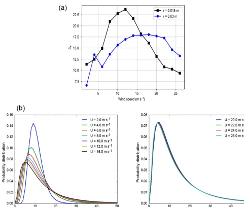
Figure 6b highlights the simulation results with an increas-ing value of the wind velocity over constant fire intensity (50 MW m−1). The results for the two different radii (0.015 and 0.030 m) are presented. The fire-spotting mechanism over varying wind speeds shows similar behaviour for the different sized firebrands. For both radii, the effective burnt area increases with increasing wind speeds, but after a cer-tain threshold an increase in the wind speed leads to a de-cline in the effective burnt area. The line plot forr=0.015 m shows that after a value of around 10 m s−1, the
Figure 6. (a)Line plot showing the sensitivity of the formulation to different wind conditions and radii when the fire intensity is constant (50 MW m−1). The measure of the effective increase in area (βe) and other simulation parameters are the same as defined in Fig. 5.(b)The line plots show the lognormal distribution for selected values of wind speedUbut constant values of fire intensityI=5000 kW m−1and firebrand radiusr=0.03 m. According to the physical parameterisation, the plots can also be interpreted as the behaviour of the lognormal distribution for varying values of the parameterσand a constant value of the parameterµ.
The lognormal distributions for selected wind speed val-ues (but fixedrandI) are plotted in Fig. 6b. These two plots show two different aspects of the response behaviour of the lognormal distribution when parameter σ is varied but pa-rameter µ is constant. Firstly, from Fig. 6b (left) it is evi-dent that with an increase in the wind speed (increasingσ, constantµ) the lognormal distribution shifts towards the left but the tails taper off slowly, making the distribution wider around the maximum. The increase in the width of the log-normal distribution leads to a larger area of “long-range” and “short-range” probability; hence, this explains the initial in-crease in the burned area in Fig. 6a. At the same time, the increasing wind speed also causes a decrease in the magni-tude of the probability; therefore, beyond a certain threshold,
the overall contribution from fire spotting starts to fall. The saturation in fire-spotting behaviour can be explained by the second aspect of the lognormal response. Figure 6b (right) shows that after a certain threshold of parameterσ or wind speed, the lognormal distributions become increasingly sim-ilar. This threshold depends upon the value of parameterµ, and for smaller values ofµ(smallerrorI) we have an early onset of this threshold. As the lognormal distributions tend to have similar probability distributions with increasing wind speed (Fig. 6b, right panel), the contribution from fire spot-ting also becomes similar and explains the saturation in the fire-spotting behaviour of the bigger firebrand radius.
σ. In terms of the physical quantities used in the parame-terisation, it can be argued that strong winds can carry the firebrands longer distances from the main source and result in a larger fire perimeter (increasing “long-range probabil-ity”). Historically it has been reported that strong winds cou-pled with extremely dry conditions formed the perfect recipe for long-range fire spotting. Strong wind speeds can loft the smaller firebrands longer distances, but with an increasing wind speed the combustion process quickens and the fire-brands reach the ground at a lower temperature. This fact ex-plains the reduced effect of fire spotting on the burned area at high wind conditions. Conversely, a larger firebrand size can sustain longer in the atmosphere which means that their “long-range” probability is relatively higher than for smaller firebrands. This explains the onset of maximum burned area at 15 m s−1instead of 12 m s−1for the 0.015 m radius. The heavier mass of bigger firebrands restricts their flight to shorter distances in comparison to the lighter firebrands and a lower magnitude of the burned area is therefore observed. The longer saturation in firebrand activity for the larger fire-brands is due to their ability to maintain longer in air without burning out.
6 Conclusions
A mathematical formulation complete with its physical pa-rameterisation RandomFront 2.3 to reproduce/mimic fire-spotting behaviour is presented in this article. In particu-lar, we provide a versatile probabilistic model for fire spot-ting that is suitable for implementation as a post-processing scheme at each time step in any of the existing operational large-scale wildfire propagation models, without calling for any major changes in the original framework. This simple physical parameterisation is also an added advantage for real-time application. In this respect, RandomFront 2.3 is implemented in the coupled fire–atmosphere model WRF-SFIRE, and a simple test case is discussed. Moreover, the proposed formulation and parameterisation can be extended to include further variables such as moisture, spatial distri-bution of combustible, orography in addition to atmospheric variables such as wind and pressure that are available by run-ning the simulation with WRF-SFIRE. This allows for an ex-amination of the interaction between the concurrent factors in wildfires.
Furthermore, simulations with a simple propagation model based on the level set method, namely LSFire+, are per-formed to highlight the different responses of the model to varying fire intensities and wind conditions, and constant cli-matic conditions are assumed throughout the entire set-up. Results using different firebrand radii are also shown.
In both implementations, i.e. WRF-SFIRE andLSFire+, the simulations are simplified to highlight the physical appli-cability of the model.
The parameterisation RandomFront 2.3 provides a simple yet versatile addition to operational fire spread models repro-ducing the different physical aspects of the firebrand landing behaviour and simulating the occurrence of secondary fires as a result. The new secondary fires are also capable of mod-ulating the weather around the primary fire and clear inter-actions between the two are observed. The wind conditions and fire-perimeter play an important role in determining the occurrence of the secondary fires.
The results highlight that the parameterisation is success-ful in reproducing the different physical aspects of firebrand landing behaviour. In this model, the complexities related to the shape and density of the firebrands are not considered and for brevity they are assumed to be spherical with a diam-eter in the order of the “collapse diamdiam-eter”. The model also does not include an explicit computation of the time taken to reach the charred oxidation state, although a heating-before-burning mechanism is introduced in the mathematical formu-lation to serve a similar purpose. The inferences made from the simulations clearly fit within the physical aspects of the fire-spotting process. The increase in the wind speed causes an initial flare-up in the fire perimeter, but in really high wind conditions the wind enhances the propagation of the main fire and this reduces the effective contribution of fire spotting. Similarly, with increasing fire intensities, the fire intensity enhances the ROS of the main fire such that new ignitions of the unburned fuel ahead of the main fire by fire spotting are reduced.
Whilst many other studies focus on the long range landing distributions of the firebrands, most of them include rigorous computational aspects like LES which limit their applicabil-ity to the operational models for wildfire propagation. The simple yet powerful probabilistic formulation presented in this paper obeys the physical aspects of the fire-spotting pro-cess and provides scope for its applicability to operational fire spread models.
Code availability. The codeLSFire+is developed in C and For-tran where the model RandomFront 2.3 acts as a post-processing routine at each time step in a LSM code for the front propa-gation implemented usingLSMLIB (Chu and Prodanovi´c, 2009); the ROS is computed using theFireLiblibrary (Bevins, 1996). The numerical libraryLSMLIBis written in Fortran2008/OpenMP and propagates the fire line through standard algorithms for the LSM, including the fast marching method algorithms. Further-more, the RandomFront 2.3 routine has also been implemented in the latest released version of WRF-SFIRE (https://github.com/ openwfm/wrf-fire/, last access: 19 December 2018) by introducing new ad hoc routines. Both implementations of RandomFront 2.3 in LSFire+and WRF-SFIRE are freely available at the official git repository of BCAM, Bilbao (https://gitlab.bcamath.org/atrucchia/ randomfront-wrfsfire-lsfire, last access: 19 December 2018).
Each simulation that spanned 20 min of physical time took about 100 min of computational time.
Simulations using LSFire+were performed over the HYPA-TIA cluster of BCAM, Bilbao, using OpenMP shared memory par-allelism, running over 24 cores inside an Intel(R) Xeon(R) CPU E5-2680 v3 2.50GHz node with 128GB RAM. The computational time for each simulation, which spanned 140 min of physical time, was about 45 min.
Eighty percent of the computational cost in both cases, i.e. WRF-SFIRE andLSFire+, was due to the post-processing routine Ran-domFront 2.3. Computational time can be reduced in the future through further code optimisation.
Author contributions. The research was planned and coordinated by GP in collaboration with IK. GP and IK formulated the physi-cal parameterisation. IK performed the simulations of the test cases usingLSFire+and was the main contributor with respect to writ-ing the text. AT implemented the RandomFront 2.3 routines into WRF-SFIRE and performed the corresponding simulations. AB contributed to running the LSFire+ simulations, and VE con-tributed to running the WRF-SFIRE simulations.
Competing interests. The authors declare that they have no conflict of interest.
Acknowledgements. This research was supported by the Basque Government through the BERC 2014–2017 and BERC 2018– 2021 programs. It was also funded by the Spanish Ministry of Economy and Competitiveness MINECO via the BCAM Severo Ochoa SEV-2013-0323 and SEV-2017-0718 accreditations, the MTM2013-40824-P “ASGAL” and MTM2016-76016-R “MIP” projects, and the PhD grant “La Caixa 2014”. The research began and was primarily developed at BCAM, Bilbao, during the postdoc fellowship of Inderpreet Kaur and the internship period of Anton Butenko.
Edited by: Tomomichi Kato
Reviewed by: two anonymous referees
References
Albini, F. A.: Spot fire distance from burning trees: a predictive model, Technical Report INT-56, U.S. Department of Agricul-ture Forest Service Intermountain Forest and Range Experiment Station, 1979.
Albini, F. A.: Potential Spotting Distance from Wind-Driven Sur-face Fires, Research Paper INT-309, U.S. Department of Agricul-ture Forest Service Intermountain Forest and Range Experiment Station, 1983.
Alexander, M. E.: Calculating and interpreting forest fire intensities, Can. J. Bot., 60, 349–357, 1982.
Anderson, H. E.: Aids to determining fuel models for estimating fire behavior. General Technical Report INT-122, Tech. rep., In-termountain Forest and Range Experiment Station, Ogden, UT, 1982.
Andrews, P. and Chase, C.: BEHAVE: Fire behavior prediction and fuel modeling system: BURN subsystem, part 2, Research Paper INT-260, USDA Forest Service, Intermountain Forest and Range Experiment Station, Ogden, Utah 84401, 1989.
Baum, H. and McCaffrey, B.: Fire induced flow field – theory and experiment, in: The Second International Symposium on Fire Safety Science, 13–17 June 1988, Tokyo, Japan, edited by Waka-matsa, T., International Association for Fire Safety Science, Lon-don, UK, 129–148, 1989.
Bevins, C. D.: FireLib: User Manual and Technical Reference, US Forest Service, Missoula Fire Sciences Laboratory, Fire Behavior Research Work Unit Systems for Environmental Management, last access: https://www.frames.gov/catalog/935 (last access: 16 August 2018), 1996.
Bhutia, S., Jenkins, M. A., and Sun, R.: Comparison of Fire-brand Propagation Prediction by a Plume Model and a Coupled– Fire/Atmosphere Large?Eddy Simulator, J. Adv. Model. Earth Syst., 2, 4, https://doi.org/10.3894/JAMES.2010.2.4, 2010. Byram, G. M.: Combustion of Forest Fuels, in: Forest Fire: Control
and Use, edited by: Davis, K. P., McGraw Hill, New York, 61–89, 1959.
Chatto, K. and Tolhurst, K. G.: A review of the relationship be-tween fireline intensity and the ecological and economic effects of fire, and methods currently used to collect fire data, Tech. Rep. 67, Fire Management Department of Sustainability and En-vironment, Victoria, 2004.
Chu, K. T. and Prodanovi´c, M.: Level set method library (LSM-LIB), available at: http://ktchu.serendipityresearch.org/software/ lsmlib/ (last access: 16 August 2018), 2009.
Coen, J. L., Cameron, M., Michalakes, J., Patton, E. G., Riggan, P. J., and Yedinak, K. M.: WRF-Fire: coupled weather-wildland fire modeling with the weather research and forecasting model, J. Appl. Meteor. Climat., 52, 16–38, https://doi.org/10.1175/JAMCD-12-023.1, 2012.
El Houssami, M., Mueller, E., Thomas, J. C., Simeoni, A., Filkov, A., Skowronski, N., Gallagher, M. R., Clark, K., and Kremens, R.: Experimental procedures characterising firebrand generation in wildfires, Fire Technol., 52, 731–751, 2016.
Fernandez-Pello, A. C.: Wildland fire spot ignition by sparks and firebrands, Fire Safety J., 91, 2–10, 2017.
Filippi, J. B., Morandini, F., Balbi, J. H., and Hill, D.: Discrete event front tracking simulator of a physical fire spread model, Simula-tion, 86, 629–646, 2009.
Finney, M.: FARSITE: fire area simulator – model development and evaluation, Research Paper RMRS-RP-4, USDA Forest Service, Rocky Mountain Research Station, Ogden, Utah, 1998. Hage, K. D.: On the dispersion of large particles from a 15-m source
in the atmosphere, J. Appl. Meteor., 18, 534–539, 1961. Himoto, K. and Tanaka, T.: Transport of disk-shaped firebrands in
a turbulent boundary layer, in: The Eighth International Sym-posium on Fire Safety Science, 18–23 September 2005, Bei-jing, China, edited by: Gottuk, D. and Lattimer, B., International Association for Fire Safety Science: Baltimore, MD, 433–444, 2005.
Sauvage, S., Sánchez-Pérez, J. M., and Rizzoli, A. E., 384– 391,2016.
Kaur, I., Mentrelli, A., Bosseur, F., Filippi, J. B., and Pagnini, G.: Wildland fire propagation modelling: A novel approach reconcil-ing models based on movreconcil-ing interface methods and on reaction-diffusion equations, in: Proceedings of the International Confer-ence on Applications of Mathematics 2015, Prague, Czech Re-public, 18–21 November 2015, edited by: Brandts, J., Korotov, S., Kˇrížek, M., Segeth, K., Šístek, J., and Vejchodský, T., Insti-tute of Mathematics – Academy of Sciences, Czech Academy of Sciences, Prague, Czech Republic, 85–99, 2015.
Kaur, I., Mentrelli, A., Bosseur, F., Filippi, J.-B., and Pagnini, G.: Turbulence and fire-spotting effects into wild-land fire simu-lators, Commun. Nonlinear Sci. Numer. Simul., 39, 300–320, 2016.
Koo, E., Pagni, P., and Linn, R.: Using FIRETEC to describe fire-brand behavior in wildfires, in: The Tenth International Sympo-sium of Fire and Materials, San Francisco, CA, 29–31 January 2007, Interscience Communications, London, UK, 2007. Koo, E., Pagni, P. J., Weise, D. R., and Woycheese, J. P.: Firebrands
and spotting ignition in large-scale fires, Int. J. Wildland Fire, 19, 818–843, 2010.
Kortas, S., Mindykowski, P., Consalvi, J. L., Mhiri, H., and Por-terie, B.: Experimental validation of a numerical model for the transport of firebrands, Fire Safety J., 44, 1095–1102, 2009. Mandel, J., Beezley, J. D., and Kochanski, A. K.:
Cou-pled atmosphere-wildland fire modeling with WRF 3.3 and SFIRE 2011, Geosci. Model Dev., 4, 591–610, https://doi.org/10.5194/gmd-4-591-2011, 2011.
Mandel, J., Amram, S., Beezley, J. D., Kelman, G., Kochan-ski, A. K., Kondratenko, V. Y., Lynn, B. H., Regev, B., and Vejmelka, M.: Recent advances and applications of WRF–SFIRE, Nat. Hazards Earth Syst. Sci., 14, 2829–2845, https://doi.org/10.5194/nhess-14-2829-2014, 2014.
Manzello, S. L., Cleary, T. G., Shields, J. R., and Yang, J. C.: On the ignition of fuel beds by firebrands, Fire Mater., 30, 77–87, https://doi.org/10.1002/fam.901, 2006.
Manzello, S. L., Maranghides, A., and Mell, W. E.: Firebrand gener-ation from burning vegetgener-ation, Int. J. Wildland Fire, 16, 458–462, 2007.
Manzello, S. L., Shields, J. R., Cleary, T. G., Maranghides, A., Mell, W. E., Yang, J. C., Hayashi, Y., Nii, D., and Kurita, T.: On the development and characterization of a firebrand generator, Fire Safety J., 43, 258–268, 2008.
Manzello, S. L., Maranghides, A., Shields, J. R., Mell, W. E., Hayashi, Y., and Nii, D.: Mass and size distribution of firebrands generated from burning Korean pine (Pinus koraiensis) trees, Fire Mater., 33, 21–31, 2009.
Martin, J. and Hillen, T.: The Spotting Distribution of Wildfires, Appl. Sci., 6, 177–210, 2016.
Mentrelli, A. and Pagnini, G.: Modelling and simulation of wildland fire in the framework of the level set method, Ricerche Mat., 65, 523–533, 2016.
Muraszew, A.: Firebrand phenomena, Aerospace Report ATR-74(8165-01)-1, The Aerospace Corp., El Segundo, CA, 1974. Niemela, J. J. and Sreenivasan, K. R.: Turbulent convection at high
Rayleigh numbers and aspect ratio 4, J. Fluid Mech., 557, 411– 422, 2006.
Pagnini, G.: A model of wildland fire propagation including random effects by turbulence and fire spotting, in: Proceedings of XXIII Congreso de Ecuaciones Diferenciales y Aplicaciones XIII Con-greso de Matemática Aplicada, Castelló, Spain, 9–13 September 2013, 395–403, 2013.
Pagnini, G.: Fire spotting effects in wildland fire propagation, in: Advances in Differential Equations and Applications, edited by: Casas, F. and Martínez, V., SEMA SIMAI Springer Series, vol. 4, Springer International Publishing Switzerland, 203–214, https://doi.org/10.1007/978-3-319-06953-1_20, 2014.
Pagnini, G. and Massidda, L.: Modelling turbulence effects in wild-land fire propagation by the randomized level-set method, Tech. Rep. 2012/PM12a, CRS4, Pula (CA), Sardinia, Italy, 2012a. Pagnini, G. and Massidda, L.: The randomized level-set method to
model turbulence effects in wildland fire propagation, in: Mod-elling Fire Behaviour and Risk, Proceedings of the International Conference on Fire Behaviour and Risk. ICFBR 2011, Alghero, Italy, 4–6 October 2011, edited by: Spano, D., Bacciu, V., Salis, M., and Sirca, C., 126–131, 2012b.
Pagnini, G. and Mentrelli, A.: Modelling wildland fire propagation by tracking random fronts, Nat. Hazards Earth Syst. Sci., 14, 2249–2263, https://doi.org/10.5194/nhess-14-2249-2014, 2014. Pagnini, G. and Mentrelli, A.: The randomized level set method
and an associated reaction-diffusion equation to model wildland fire propagation, in: Progress in Industrial Mathematics at ECMI 2014, edited by: Russo, G., Capasso, V., Nicosia, G., and Ro-mano, V., vol. 22, Mathematics in Industry, Springer, Cham, pro-ceedings of The 18th European Conference on Mathematics for Industry, ECMI 2014, Taormina, Italy, 9–13 June 2014, 531–540, 2016.
Pereira, J. C. F., Pereira, J. M. C., Leite, A. L. A., and Albuquerque, D. M. S.: Calculation of spotting particles maximum distance in idealised forest fire scenarios, J. Combust., 2015, 513576, https://doi.org/10.1155/2015/513576, 2015.
Perryman, H. A., Dugaw, C. J., Varner, J. M., and Johnson, D. L.: A cellular automata model to link surface fires to firebrand lift-off and dispersal, Int. J. Wildland Fire, 22, 428–439, 2013. Porterie, B., Zekri, N., Clerc, J.-P., and Loraud, J.-C.: Modeling
for-est fire spread and spotting process with small world networks, Combust. Flame, 149, 63–78, 2007.
Pugnet, L., Chong, D., Duff, T., and Tolhurst, K.: Wildland–urban interface (WUI) fire modelling using PHOENIX Rapidfire: A case study in Cavaillon, France, in: MODSIM2013, 20th Inter-national Congress on Modelling and Simulation, Modelling and Simulation Society of Australia and New Zealand, December 2013, edited by: Piantadosi, J., Anderssen, R., and Boland, J., 228–234, 2013.
Sardoy, N., Consalvi, J. L., Porterie, B., and Fernandez-Pello, A. C.: Modeling transport and combustion of firebrands from burning trees, Combust. Flame, 150, 151–169, 2007.
Sardoy, N., Consalvi, J. L., Kaiss, A., Fernandez-Pello, A. C., and Porterie, B.: Numerical study of ground-level distribution of fire-brands generated by line fires, Combust. Flame, 154, 478–488, 2008.
Sethian, J. A. and Smereka, P.: Level set methods for fluid inter-faces, Ann. Rev. Fluid Mech., 35, 341–372, 2003.
Tech-nical Note NCAR/TN-475+STR, NCAR, Mesoscale and Mi-croscale Meteorology Division, Boulder, Colorado, USA, 2008. Tarifa, C., del Notario, P., and Moreno, F.: On flight paths and
life-times of burning particles of wood, in: 10th Symposium on Com-bustion, 17–21 August 1964, Cambridge, UK, The Combustion Institute, Pittsburgh, PA, 1021–1037, 1965.
Tarifa, C., del Notario, P., Moreno, F., and Villa, A.: Transport and combustion of firebrands, Technical Report Grants FG-SP-114, FG-SP-146, Instituto Nacional de Tecnica Aeroespacial, 1967. Thomas, J. C., Mueller, E. V., Santamaria, S., Gallagher, M., El
Houssami, M., Filkov, A., Clark, K., Skowronski, N., Hadden, R. M., Mell, W., and Simeoni, A.: Investigation of firebrand gen-eration from an experimental fire: Development of a reliable data collection methodology, Fire Safety J., 91, 864–871, 2017. Thurston, W., Kepert, J. D., Tory, K. J., and Fawcett, R. J. B.: The
contribution of turbulent plume dynamics to long-range spotting, Int. J. Wildland Fire, 26, 317–330, 2017.
Tohidi, A. and Kaye, N. B.: Stochastic modeling of firebrand shower scenarios, Fire Safety J., 91, 91–102, 2017.
Tohidi, A., Kaye, N., and Bridges, W.: Statistical description of fire-brand size and shape distribution from coniferous trees for use in Monte Carlo simulations of firebrand flight distance, Fire Safety J., 77, 21–35, 2015.
Tolhurst, K., Shields, B., and Chong, D.: Phoenix: Development and Application of a Bushfire Risk Management Tool, Aust. J. Emerg. Manage., 23, 47–54, 2008.
Tymstra, C., Bryce, R., Wotton, B., Taylor, S., and Armitage, O.: evelopment and structure of Prometheus: the Canadian wild land fire growth simulation model, Information Report NOR-X-417, Canadian Forest Service, Northern Forestry Centre, 2010. Wadhwani, R., Sutherland, D., Ooi, A., Moinuddin, K., and Thorpe,
G.: Verification of a Lagrangian particle model for short-range firebrand transport, Fire Safety J., 91, 776–783, 2017.
Wang, H. H.: Analysis on downwind distribution of firebrands sourced from a wildland fire, Fire Technol., 47, 321–340, 2011. Woycheese, J. P., Pagni, P., and Liepmann, D.: Brand propagation