UDK 519.682:519.85:624.073
Uporaba programa MATHEMATICA v metodi končnih elementov za izračun tankih plošč
The Use of Program MATHEMATICA in the Finite Element Method for Thin Plate Analysis
MATJAŽ SKRINAR
Prispevek prikazuje uporabo programa MATHEMATICA v metodi končnih elementov. S programom smo izpeljali celoten izračun togostne matrike in obtežnega vektorja elementa po metodi deformacije za tanke plošče. Element ima 9 vozlišč s štirimi prostostnimi stopnjami v vozlišču, torej skupaj 36 prostostnih stopenj. S tako izbiro prostostnih stopenj smo dosegli zveznost C ,. Ker v uporabljeni literaturi zanj nismo našli označbe, smo mu dodelili označbo H9. Element smo testirali na dveh numeričnih primerih in dobljene rezultate primerjali s točnimi vrednostmi, znanimi iz literature, kakor tudi z rezultati, dobljenimi z izračuni z elementi z manjšim številom prostostnih stopenj (element BFS).
The article presents the use of the program MATHEMATICA in the finite element method. The entire computation of the stiffness matrix and load vector was computed with the program. Such an element has 9 node points with four degrees of freedom per node, that is 36 degrees of freedom. Such a choice of degrees of freedom achieves Ci continuity. Because a name for such an element was not found in the literature, it was named H9. The element was tested with numerical examples and the obtained result were compared with exact values and with result obtained by computation with elements with lower value degrees of freedom (element BFS1.
0. PREDSTAVITEV PROGRAMA
Program MATHEMATICA je programski pa ket, ki je zlasti namenjen za uporabo v matematiki, čeprav ga je mogoče koristno uporabiti v mnogih inženirskih problemih, saj ponuja uporabniku širo ko paleto možnosti. Odlikuje ga zmožnost simbo ličnega operiranja s podatki. Mnoge naloge je nam reč mogoče tako reševati analitično in ne samo numerično.
1. PREDSTAVITEV PROBLEMA
Metoda končnih elementov je dandanes ena izmed najbolj razširjenih in uporabnih numeričnih metod, ki se uporabljajo v konstrukterski inže nirski praksi. Konstrukcijo, ki jo želimo prera čunati, diskretiziramo v končno število elementov in za vsakega izmed njih izračunamo lokalno to- gostno matriko. Prav računanje togostne matrike elementa je ena od najzahtevnejših operacij, ki porabi največ časa za računanje, še posebej če matriko vsakega elementa numerično integriramo. Kadar se odločimo, da bomo za diskretizacijo konstrukcije uporabili enake vrste elementov (ni nujno tudi enakih velikosti), je primerno takšno matriko ovrednotiti simbolično z integriranjem po ploskvi oz. prostornini elementa.
Ta operacija integriranja pa ni toliko zapletena kakor obsežna naloga, saj pride pri izračunu matrik z večjim številom prostostnih stopenj do množice podatkov, ki vodijo v nepreglednost. Upoštevajoč še človeško nagnjenost k zmotam je sklep ta, da je treba tak izračun prepustiti natančnejšemu izva jalcu - računalniku. Zaradi zmožnosti analitičnega odvajanja, integriranja ter drugih pomembnih mo žnosti, smo se odločili, da s programom MATHE MATICA izračunamo togostno matriko pravokotne ga elementa. Namen tega izračuna ni v prvi vrsti pridobitev togostne matrike, temveč prikaz mož nosti uporabe v konstrukterskem področju.
0. AN INTRODUCTION OF THE PROGRAM
Program Mathematica is a software package which is intended in the first place for use in mathematics, although its capabilities could also be applied to enginering problems because of its wide specter of functions. One of its best points is its capability of symbolic handling of data. Many tasks can thus be solved in a strictly symbolic way and not only numerically.
1. AN INTRODUCTION OF THE PROBLEM
The finite element method is today one of the most widespread and useful methods in engine ering practice. A structure which is to be analy zed is discretised into a finite number of elements and the local stiffness matrix must be calculated for each of them. The calculation of the stiffness matrix of the element is one of the most exacting operations and requires most of the computing time, especially if the matrix for each element is integrated numerically. If a decision is made to use the equal type of the element for the discreti sation of the structure, it is suitable to valuate such a stiffness matrix in symbolic form with integration over the area or the volume in the element.
2. TEORETIČNE OSNOVE 2. TEORETICAL BACKGROUND
Osnovne enačbe, ki so znane iz mehanike, so privzete iz [11.
Na element je vezan pravokoten kartezijev koordinatni sistem, katerega osi sta vzporedni z robovi plošče. Izhajamo iz izhodiščne predpostavke, da linijski element, ki je bil pred deformacijo pra vokoten na ravnino plošče, ostane po deformaciji nespremenjen po dolžini in pravokoten na srednjo deformirano ravnino plošče (Kirchhoff-ova pred postavka). Ta teorija, postavljena že leta 1850, opisuje obnašanje plošče samo z upogibom osrednje ravnine. Upogib le-te je funkcija dveh med seboj pravokotnih koordinat v ravnini plošče. Glede na to predpostavko je naša analiza v dvodimenzional nem področju. Zapišemo lahko:
Basic equations from mechanics are taken from 111.
A Cartesian coordinate system is attached to the element, with axes parallel to the boundaries of the plate. We start from the assumption that there is no deformation in the middle plane of the plate and that points lying initially on a normal to middle plane of the plate remain on the normal to middle surface of the plate after deformation (Kirchoff’s hypothesis). This classical theory established in 1850 describes the behavior of pla tes only with the deflection of the middle surface of the plate. This deflection is a function of two orthonormal coordinates in the middle surface of the plate. According to this assumption, our analy sis lies in a two dimensional area. We can write:
f 9w . 9 i v
w = w ( X, v), u = - z —— in v = - z —— (1).
9 A' 9
v
Komponente deformacijskega tenzorja so: The components of the strain tensor are:
9" w n 3 W
0 3 W “ “ 9 A-9 y
0 rr 3 92 iv 0
Zjz
3 A'By 9 y 2
0 0 0 _
(2) .
Končni element je po tlorisni obliki pravokot nik. Število vozliščnih točk na elementu je devet, njihova lokacija je naslednja: štiri vogalne točke, štiri točke na sredini stranic pravokotnika in sre dinska točka (sl. 1).
Sl. 1. Vozliščne točke in izbrane prostostne stopnje.
Fig. 1. The nodal points and chosen degrees of freedom.
The shape of the finite element is rectangle. The number of nodes is 9. They are located as follows: four corner points, four points on the midside nodes and the centroidal point (Fig. 1).
Zaradi zagotovitve čim večje natančnosti za glavne neznanke v vozliščih izberemo pomik iv, prva odvoda 3 iv /9 x in 9 iv /3 y, (ki sta soraz merna zasukoma 6 X in 0 V) ter mešani odvod
92 w / d x d y ; torej imamo v Vozlišču 4 prostostne
stopnje oziroma 36 prostostnih stopenj v celotnem elementu. Vektor neznak v vozlišču »i« zapišemo kot:
I
W \
« 0.V 1 ■ \ , b e
>-\ 9" w/3.\'9y /
To achieve better accuracy, four unknowns in the nodes are next chosen: displacements w, first derivates 9 iv /9 a-and 9 iv /9 y (which are propor tional to the rotations 0 Y in 0 V.) and mixed deri vative 92iv/9.v3y. According to" chosen unknowns we have 4 degrees of freedom per node or 36 de grees of freedom per total element. The vector of the unknowns in the joint can be written as:
Vrednosti a 0 X in b Qv sta uvedeni zato, da postane vektor neznanih količin dimenzionalno homogen.
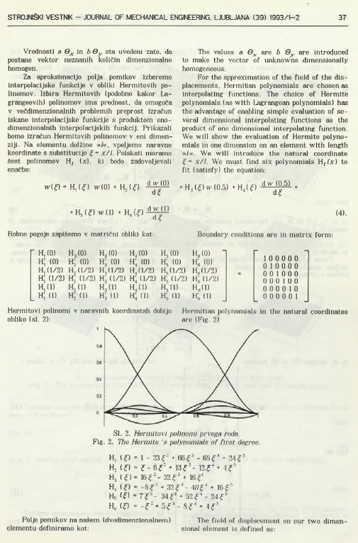
Za aproksimacijo polja pomikov izberemo interpolacijske funkcije v obliki Hermitovih po linomov. Izbira Hermitovih (podobno kakor La- grangeovih) polinomov ima prednost, da omogoča v večdimenzionalnih problemih preprost izračun iskane interpolacijske funkcije s produktom eno dimenzionalnih interpolacijskih funkcij. Prikazali bomo izračun Hermitovih polinomov v eni dimen ziji. Na elementu dolžine »/«, vpeljemo naravne koordinate s substitucijo ? = x /l. Poiskati moramo šest polinomov Hy Ly), ki bodo zadovoljevali
enačbo:
w(?) = H, ( ?) w(0) + H2(?) d ^ f0)
The values a 0 V are b Qv are introduced to make the vector of unknowns dimensionally homogeneous.
For the approximation of the field of the dis placements, Hermitìan polynomials are chosen as interpolating functions. The choice of Hermite polynomials (as with Lagrangean polynomials) has the advantage of enabling simple evaluation of se veral dimensional interpolating functions as the product of one dimensional interpolating function. We will show the evaluation of Hermite polyno mials in one dimension on an element with length »/«. We will introduce the natural coordinate ? = x /l. We must find six polynomials Hj(x) to fit (satisfy) the equation:
-H 3(<f)w(0,5) + H4(?) ■^ g d(P’5)' +
+ H5(?) w( 1) + H6(?) (4).
Robne pogoje zapišemo v matrični obliki kot: Boundary conditions are in matrix form:
" H,(0) H2(0) Ha (0) h4 (0) H5 (0) H6(0) " 1 n n n n n
h; (0) h; (0) h; (o) h; (0) h; to) H’g (0) n l 0 0 0 0 0 1 n n n n H, (1/2) H2 (1/2) H3(l/2) H4(l/2) H5(1/2) H6(l/2) _ U 0 0 1 0 0 01 u u u u
H (1/2) H’ (1/2) h; (1/2) h; (1/2) h; (1/2) h; (1/2) 0 0 0 1 0 0
H,(l) H2 (1) h3(1) h4 (1) H5(l) H6(l) 0 0 0 0 1 0
h; (d H’ (1) h; (d h; tu h; (d H’s (1) 0 0 0 0 0 1
Hermitovi polinomi v naravnih koordinatah dobijo Hermitian polynomials in the natural coordinates
obliko (si. 2): are (Fig. 2)
0,8
0,6
OA
0,2
0
SI. 2. Hermitovi polinomi prvega reda.
Fig. 2. The Hermite ’s polynomials of first degree.
H, (?) = 1 - 2 3 ?2 + 6 6 ?3 - 68 ? 4 + 2 4 ? 5 H, (?) = ? - 6 ? 2 + 13?3- 12?4 + 4 ? 5 H3 (? ) = 16?2- 32 ? 3 + 16?4
H4 (?) = - 8 ? 2 + 32 ? 3- 40 ? 4 + 16?5 H5 (?) = 7 ? 2- 34? 3 + 5 2 ? 4 - 2 4 ? s H6 (?) = - ? 2 + 5 ? 3 - 8 ? 4 + 4 ? 5
Polje pomikov na našem (dvodimenzionalnem) The field of displacement on our two
w = w(,f, 77) = N (£ 77) q (5),
kjer velja: where:
r] = y/1, naravna koordinata v smeri osi y, r\ = y/I, the natural coordinate in y direction,
9 = iQv 9s- - 9 9]T vektor vozliščnih pomikov q= [9,, q2, q3, ...9 9] > vector of modal
displace-oziroma neznank (3), ments (3),
N (£ 77), matrika interpolacijskih funkcij v obliki: N ((£ 77), the matrix of the interpolating functions:
N ( £9) = [ N , , N 2, .... N9] (6K
Vsaka izmed podmatrik N[ (i = 1, 2, 9) ustreza enemu vozlišču in ima štiri elemente:
II
SB
1
1
z N 12 n21 n22]
N2= 1[ n31 N32 n41 n42] N3=i[n51 n52 N61 n62]
Z £- II
> , 3 n14 n23 n24]
N9 = [ N 55 kjer velja:
N f j - H , in so H j (£) in Hy- (77) Hermitovi polinomi spre
menljivk f in 77.
Na sliki 3 so prikazane interpolacijske funk cije za vogalno vozlišče, vozlišče na sredini roba in osrednje vozlišče.
Zveza med vektorjem deformacije X in vek
torjem osnovnih neznanih količin v vozlišču je podana z izrazom:
X =
-ki ob vpeljavi (5) in (6) postane:
Each of the sub matrixes N[ (i = 1, 2,..., 9) belongs to one node and it has four elements:
N5 - I [ n33 n34 n43 n44]
N8 - I[ n53 n54 n63 n64]
n7 = I[ n15 N 16 n25 n26]
n8 = [ n35 n36 n45 n46]
56 ^65 ^66 (7),
where:
0 h, ( n ) ( 8 )
Hy (£) and (77) are Hermitian polynomials of variables f in 77, respectively.
Fig. 3 shows the interpolating function for the corner node, midside node and central node.
The relation between the vector of deforma tion X and the vector of the unknows in joint is
given by the expression:
1 92 w
9
a 9 f 2
1 92 w
b2 9 q2
2 92 w
ab
Introducing Eq. (5) and Eq. (6) it follows:
kjer so:
X =
B, =
1 92N
a~ 3 f 2
1 92N
b 2 9 T)2
2 92N
ab 9 f 9n
1 9 2 N y 2
a 9 f 2
1 9 2 N y
b 2 3 r
2 9 2 N y
ab 3 f 39
q = B q = [j5, B2, ... , ß 9]
where
(10) ,
Sl. 3. Interpolacijske funkcije vogalne, robne in sredinske točke.
Fig. 3. The interpolating functions for the corner node, midside node and the middle point.
Togostno matriko elementa oblikujemo iz po- The element stiffnes matrix is formed from: sameznih podmatrik:
K = [ k j j l / , 7 = 1 , 2 ...9 (12),
kjer so: 1 1 where
k j j = ab J J ß / T (£ n ) D B j i l /?)d(fd?7 13)
o o
in je D matrika koeficientov elastičnosti: and D is the matrix of elastic coefficients.
12(1-v 2)
Podobno izračunamo vektor posplošenih sil v vozlišču i, ki je funkcija površinske razdelitve obtežbe po elementu:
0 0 v 0 1 0
1- v (14).
1 1
Q, = a b
J J
NyTp d <f d p0 0
Notranje statične količine izračunamo z: The element forces are evaluated by:
M - D B q
(15) .
(16) .
3. IZRAČUN MATRIK k u IN Q, ZA ELEMENT H9
3. THE COMPUTATION OF MATRIX
k u AND Qj FOR THE ELEMENT H9
Ukaze programu MATHEMATICA podajamo na dva načina: bodisi neposredno v programu, torej iterativno, bodisi prek vhodne datoteke, kamor zapišemo ukaze v isti obliki, kakor bi to storili neposredno v programu.
Drugi način je vsekakor boljši, saj omogoča lažje spreminjanje vhodnih podatkov, dodajanje ko mentarjev in celovitejši pregled zahtevanega dela. Program zahteva strogo upoštevanje predpi sane sintakse, saj je treba dosledno uporabljati velike in male črke, tako v ukazih, kakor tudi pri uporabi spremenljivk. Vse komentarje ogradimo z oklepaji in zvezdicami - (* komentar *).
Kot primer bomo prikazali datoteko z ukazi za izračun ene izmed podmatrik k^ . Zaradi si metrije dejansko računamo samo podmatrike z indeksom j Ž j.
Datoteka za izračun podmatrike k99 je pri kazana na sliki 4.
Orders can be passed to the program Mathe matica in two ways: directly in the program, i.e. interactive, or with an input file. In such a file orders are written in the same way as they would be written directly in the program. This second way is more appropriate because of the ease of changing the input data, adding comments and for a better overview of requested tasks.
The program requires the use of the prescri bed syntax. Capital letters should be used very strictly in the order of usage of the variables. The comments are written with parentheses and asterisks — ( * the comment * ).
As an example, we will show an input file for the computation of one of the matrices k,,.
Due to the symmetry only the matrices with index j è i are computed.
The file for the computation of the submatrix kg9 is shown on the Fig. 4.
h5 [e_] = InterpolatingPolynomial [{<0,{0,0}>,{0.5,{0,0>>,{l,{l,0)}>,e] h6[e_] = InterpolatingPolynomial [{{0, {0,0>},{0.5,{0,0}},{l,{0,l}}},e]
(* definiranje Hermitovih polinomov / declaration of Hermite’s
poynimials *)
d ={<dx, d l ,0),Idi,dy,0},{0,0,dxy}}
n9 = < h 5 [ e ] * h 5 t n ) , h 5 [ e ] * h 6 [ n ] , h 6 [ e ] * h 5 [ n ] , h 6 [ e ] * h 6 [ n ] >
(* definiranje enačb 7 / equations 7 *)
b9 = - ( D [ D [ n 9 , e ] , e ) / a / a , D [ D [ n 9 , n l , n ] / b / b , 2 * D [ D [ n 9 , e ] , n ] / a / b >
(* enačbe 11 / equations 11 *)
k99 =a*b* Integrate [Integrate! Transpose [b9] ,d.b9,{e,0,l>],{n,0,l>]
(* enačbe 13 / equations 13*)
SI. 4. Vstopna datoteka (detajl).
Fig. 4. The input file (a detail).
Datoteko z ukazi podamo programu z ukazom
«imedoteke. tip.
Podobno izračunamo preostalih 44 matrik k yj reda 4*4. Program izvede zadane ukaze, vendar ne poišče avtomatično optimalne (najkrajše) oblike zapisa rezultatov.
Vse rezultate je mogoče shraniti v datoteko; na izbiro imamo več različnih oblik zapisa. Poleg standardnega zapisa so mogoči še zapisi v program skih jezikih C in Fortran ter zapis v obliki, ki jo razume urejevalnik besedila TgX. Možno je obliko vati tudi svoje oblike zapisov.
The input file is transmitted to the program with a command «filename.type.
In the similar way, the remaining 44 matrices k of order 4*4 are calculated. The program executes the given commands, but does not discover a shorter form of the result automatically.
It is possible to store all the obtained results on a file. There are several possibilities of format; in addition to the standard format, there are for mats in programming languages such as C and Fortran and a format for the text editor TgX. It is possible to create new formats.
3.1 Testni primer
Analiza kvadratne plošče z zvezno obtežbo (sl. 5). Zaradi dvoosne simetrije je dovolj analizirati samo četrtino plošče (na dveh robovih upoštevamo realne robne pogoje, na nasprotnih robovih pa sime- trijske robne pogoje = zasuk okoli roba je enak nič).
Uporabnost elementa H9 smo preizkusili na dveh primerih:
a) plošča je na obodu vpeta in
b) plošča je na obodu prosto položena.
3.1 Test Examples
The analysis of a rectangular plate with uniformly distributed load (Fig. 5). Because of the double symmetry, only one quarter of the plate was analyzed. On two boundaries, the real boun dary conditions were considered, and two of the symmetrical boundary conditions. The usefulness of the element H9 was tested in two examples:
1 2 3
4 5 6
7 8 9
Sl. 5. Kvadratna plošča: mreži končnih elementov H9 (levo) in končnih elementov BFS (desno).
Fig. 5. The square plate: the meshes of the finite elements H9 (left) and BFS finite elements (right).
Oba primera smo preračunali s programom, ki uporablja končni element s šestnajstimi pro stostnimi stopnjami. Element ima štiri vozliščne točke, ki se ujemajo z vogalnimi točkami, pro stostne stopnje v posameznem vozlišču pa so enake kakor pri elementu H9 ( w, d w / d x , 3 w/ 9 y,
92 w / d y d x ) . Po 111 ima ta element označbo BFS. Ker gre v našem primeru samo za prikaz iz peljave končnega elementa, smo pri analizi in pre verjanju uporabili zelo grobo mrežo. Pri diskretiza- ciji z elementom H9 smo uporabili en sam element , pri diskretizaciji z elementi BFS pasmo uporabili mrežo 2*2 elementa. Tako smo pri obeh mrežah dobili devet računskih točk, v katerih smo primer jali vrednosti pomikov in obeh zasukov (sl. 5).
Analitični izrazi za pomik sredinske točke v odvisnosti od obtežbe in fizikalnih parametrov plošče so podani v [11 (stran 280, tabela 8.2).
Za testni primer smo izbrali naslednje po datke:
/ = 2 m — razpon celotne plošče,
h = 0,1 m — debelina plošče,
E = 3.107 kN /m 2 — modul elastičnosti v = 0,3 — Poissonov koeficient,
q = 10 kN/m 2 * — zvezna obtežba plošče.
1. primer
Plošča je na obodu vpeta. Analitična vrednost pomika v sredini plošče (točka 9) je 0,0733824 mm 111. Rezultati analize so podani v preglednici 1.
2. primer
Plošča je na obodu prosto položena. Analitična vrednost pomika v sredini plošče (točka 9) je 0,2364544 mm (11. Rezultati analize so podani v preglednici 2.
Kakor je razvidno iz preglednic 1 in 2, je en sam element H9 pri analizi vpete plošče dosegel malenkostno boljše rezultate kakor mreža štirih elementov BFS. Nasprotno pa je element H9 do segel pri prosto položeni plošči nekoliko slabše rezultate. Šele analiza konstrukcije, diskretizirane z gostejšo mrežo, bi dala pravi odgovor na vpra šanje o večji ustreznosti elementa H9 v primerjavi z elementom BFS; vendar to presega obseg tega prispevka.
Both examples were computed with a program that uses a finite element with 16 degrees of free dom. This element has four nodal points that coin cide with the corners and the degrees of freedom in each node are equal to the degrees of freedom for element H9 (w, dw/ dx, dw/ dy, 32w/ dy dx) .
According to (11 this element is classified as BFS. Because the purpose of this paper is to pre sent the development of the new finite element, a very rough mesh was used. In the discretization with element H9, only one element was used and in the discretization with elements BFS, a mesh of 2*2 elements was used. In both cases, 9 computing points were obtained in which the va lues of the displacements and rotations were com pared (Fig. 5).
Analytical results depending on the physical parameters of the plate and the given load are given in (11 (page 280, table 8.2).
For testing data values were next chosen:
1 = 2 m — the span of the whole plate
h = 0,1 m — the thickness of the plate
E = 3.107 kN /m 2 — the elasticity module v = 0,3 — the Poisson’ s ratio
q= 10 kN/m 2 — the value of the uniform load
Case 1
Clamped plate. The exact value of the deflec tion in the centre of the plate (point 9) is 0.0733824 mm 111. The results of the analysis are given in table 1.
Case 2
Simply supported plate. The exact value of the deflection in the centre of the plate (point 9) is 0.2364544 mm (11. The results of the analysis are given in table 2.
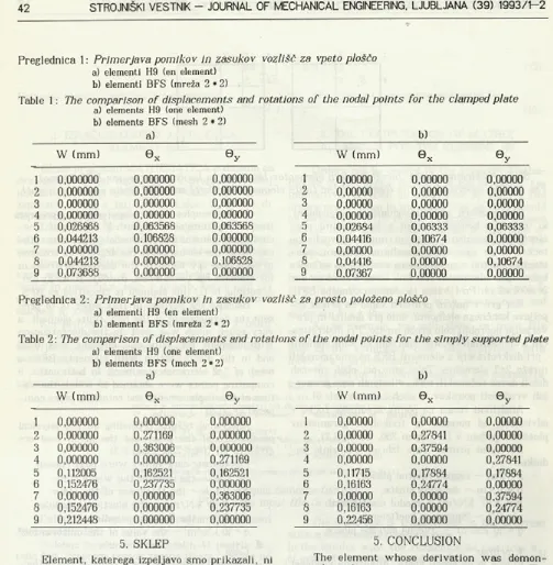
Preglednica 1: Primerjava pomikov in zasukov vozlišč za vpeto ploščo
a) elementi H9 (en element) b) elementi BFS (mreža 2 * 2 )
Table 1 : The comparison of displacements and rotations of the nodal points for the clamped plate
a) elements H9 (one element)
b) elements BFS (mesh 2 * 2 )
a) b)
W (mm) ©x 0 y W (mm) ©X Qy
1 0,000000 0,000000 0,000000 1 0,00000 0,00000 0,00000
2 0,000000 0,000000 0,000000 2 0,00000 0,00000 0,00000
3 0,000000 0,000000 0,000000 3 0,00000 0,00000 0,00000
4 0,000000 0,000000 0,000000 4 0,00000 0,00000 0,00000
5 0,026868 0,063568 0,063568 5 0,02684 0,06333 0,06333
6 0,044213 0,106828 0.000000 6 0,04416 0,10674 0,00000
7 0,000000 0,000000 0,000000 7 0,00000 0,00000 0,00000
8 0,044213 0,000000 0,106828 8 0,04416 0,00000 0,10674
9 0,073688 0,000000 0,000000 9 0.07367 0,00000 0,00000
Preglednica 2: Primerjava pomikov in zasukov vozlišč za prosto položeno ploščo
a) elementi H9 (en element) b) elementi BFS (mreža 2 * 2 )
Table 2 : The comparison of displacements and rotations of the nodal points for the simply supported plate
a) elements H9 (one element) b) elements BFS (mech 2*2)
a) b)
W (mm) ©X 0y W (mm) ©X 0y
1 0,000000 0,000000 0,000000 1 0,00000 0,00000 0,00000
2 0,000000 0,271169 0,000000 2 0,00000 0,27841 0,00000
3 0,000000 0,363006 0,000000 3 0,00000 0,37594 0,00000
4 0,000000 0,000000 0,271169 4 0,00000 0,00000 0,27841
5 0,112005 0,162521 0,162521 5 0,11715 0,17884 0,17884
6 0,152476 0,237735 0,000000 6 0,16163 0,24774 0,00000
7 0,000000 0,000000 0,363006 7 0,00000 0,00000 0,37594
8 0,152476 0,000000 0,237735 8 0,16163 0,00000 0,24774
9 0,212448 0,000000 0,000000 9 0,22456 0,00000 0,00000
5. SKLEP
Element, katerega izpeljavo smo prikazali, ni novost, zanimiv je samo način izpeljave. Prikazani način omogoča zanesljivo izpeljavo obsežnega kon čnega elementa v razmeroma kratkem času. Takšen element je z osebnim računalnikom PC 486 namreč mogoče izračunati v enem delovnem dnevu, z zmožnejšimi računalniki pa še znatno hitreje. Izračun končnega elementa s programom MATHEMATICA poleg hitrosti ponuja še točnost izračuna, saj ob pravilno podanih podatkih odpadejo vse človeške zmote pri računu. Zato lahko upra vičeno trdimo, da je tak program v konstrukter- skem delu več ko dobrodošel, njegova uporabnost pa se bo zagotovo izkazala še pri marsikaterem drugem inženirskem problemu. 5
5. LITERATURA 5. REFERENCES
111 Sekulovič, M.: Metod konačnih elemenata.
G radjevinska knjiga, Beograd, 1988
121 Wolfram, S.: Mathematica, A System of Doing Ma thematics by Computer. The Advance Book Program. 1991.
5. CONCLUSION
The element whose derivation was demon strated in this paper is not an innovation. The point of interest lies in its derivation. The pre sented way enables a precise derivation of a large finite element in short time. It is possible to de velop and compute such an element with a PC486 machine in one day of work. Such an approach offers in addition to speed, also accuracy. The use of the program Mathematica can be welcomed in the field of engineering work and its advantages are likely to apply to many other engineering problems.
Avtorjev naslov:
A uthor's Address: mag. Matjaž Skrinar, dipl. inž. Univerza v Mariboru
Tehniška fakulteta Smetanova 17 Maribor, Slovenija
Prejeto:
Received: 24.12.1992
Sprejeto: