ISSN Print: 2152-7385
DOI: 10.4236/am.2019.106030 Jun. 17, 2019 419 Applied Mathematics
Homotopy Analysis Method for Solving Initial
Value Problems of Second Order with
Discontinuities
Waleed Al-Hayani, Rasha Fahad
Department of Mathematics, College of Computer Science and Mathematics, Mosul University, Mosul, Iraq
Abstract
In this paper, the standard homotopy analysis method was applied to initial value problems of the second order with some types of discontinuities, for both linear and nonlinear cases. To show the high accuracy of the solution results compared with the exact solution, a comparison of the numerical re-sults was made applying the standard homotopy analysis method with the iteration of the integral equation and the numerical solution with the Simp-son rule. Also, the maximum absolute error, ⋅ 2, the maximum relative
er-ror, the maximum residual error and the estimated order of convergence were given. The research is meaningful and I recommend it to be published in the journal.
Keywords
Homotopy Analysis Method, Initial Value Problems, Heaviside Step Function, Dirac Delta Function, Simpson Rule
1. Introduction
Liao Shijun [1] [2] [3] proposed in 1992 in his Ph.D. dissertation a new and fruitful method (Homotopy Analysis Method (HAM)) for solving linear and nonlinear (ordinary differential, partial differential, integral, etc.) equations. It has been shown that this method yields a rapid convergence of the solutions se-ries to linear and nonlinear deterministic.
In recent literature, Al-Hayani and Casasùs [4] [5] applied the Adomian de-composition method (ADM) to the initial value problems (IVPs) with disconti-nuities. Ji-Huan [6] used the homotopy perturbation method (HPM) solving for nonlinear oscillators with discontinuities.
How to cite this paper: Al-Hayani, W. and Fahad, R. (2019) Homotopy Analysis Method for Solving Initial Value Problems of Second Order with Discontinuities. Ap-plied Mathematics, 10, 419-434.
https://doi.org/10.4236/am.2019.106030
Received: March 30, 2019 Accepted: June 14, 2019 Published: June 17, 2019
Copyright © 2019 by author(s) and Scientific Research Publishing Inc. This work is licensed under the Creative Commons Attribution International License (CC BY 4.0).
http://creativecommons.org/licenses/by/4.0/
DOI: 10.4236/am.2019.106030 420 Applied Mathematics In the consulted bibliography we have not found any results of the application of the HAM to differential problems with discontinuities. For this reason, this paper systematically analyzes its application to IVPs of ODEs of second order with independent non-continuous term. We have treated functions with a dis-continuous derivative, with some of Heaviside step function and with Dirac del-ta function.
In what follows, we give a brief review of the HAM.
2. Basic Idea of HAM
In this article, we apply the HAM to the discussed problem. To show the basic idea, we consider the following differential equation
( )
( )
,u x =k x
(2.1)
where is a nonlinear operator, x denotes independent variable, u x
( )
is an unknown function, and k x( )
is a known analytic function. For simplicity, we ignore all boundary or initial conditions, which can be treated in the similar way. By means of generalizing the traditional homotopy method, Liao [1] [2] [3] con-structs the so-called zero-order deformation equation(
1−q)
φ( )
x q u x; − 0( )
=qhH x( )
{
φ( )
x q; −k x( )
}
, (2.2) where q∈[ ]
0,1 is an embedding parameter, h≠0, is a non-zero auxiliary pa-rameter H x( )
≠0 is an auxiliary function, is an auxiliary linear operator,( )
0
u x is an initial guess of u x
( )
andφ
( )
x q; is an unknown function. It isimportant to note that one has great freedom to choose auxiliary objects such as h and in the HAM. Obviously when q=0 and q=1, both
( )
x;0 u x0( )
and( ) ( )
x;1 u xφ
=φ
= (2.3)hold. Thus as q increases from 0 to 1, the solution
φ
( )
x q; varies from theini-tial guess u x0
( )
to the solution u x( )
. Expandingφ
( )
x q; in Taylor serieswith respect to q, one has
( )
0( )
( )
1
; m,
m m
x q u x u x q
φ +∞
=
= +
∑
(2.4)where
( )
0 ;
1 ,
!
m
m m
q x q u
m q
φ
=
∂ =
∂ (2.5)
If the auxiliary linear operator, the initial guess, the auxiliary parameter h, and the auxiliary function are so properly chosen, then the series (2.4) converges at
1
q= and one has
( )
0( )
( )
1
;1 m ,
m
x u x u x
φ +∞
=
= +
∑
(2.6)DOI: 10.4236/am.2019.106030 421 Applied Mathematics
(
1−q)
φ( )
x q u x; − 0( )
+q{
φ( ) ( )
x q k x; − }
=0, (2.7)which is used mostly in the HPM [6] [7].
According to Equation (2.5), the governing equations can be deduced from the zeroth-order deformation Equations (2.2). We define the vectors
( ) ( )
( )
{
0 , 1 , ,}
.i = u x u x u xi
u (2.8)
Differentiating Equation (2.2) m times with respect to the embedding para-meter q and then setting q=0 and finally dividing them by m!, we have the so-called mth-order deformation equation
( )
1( )
(
1)
,m m m m m
u x − u − x =h −
u
(2.9)
where
(
1) ( )
1{
( )
1( )
}
0;
1 ,
1 !
m
m m m
q
q k x
m q
φ
−
− −
=
∂ − =
− ∂
u
(2.10)
and
0, 1,
1, 1.
m
m m
≤
= >
(2.11)
It should be emphasized that u xm
( )
(
m≥1)
are governed by the linear eq-uation (2.9) with the linear boundary conditions that come from the original problem, which can be easily solved by symbolic computation softwares such as Maple and Mathematica.3. HAM Applied to an IVP of the Second Order
Consider the general IVP of the second order [4]:
(
)
(
)
( )
( )
2
, , , , 0 ,
0 , 0 ,
u g u u k u f x u u x T
u u
λ
α β
′′+ ′ + = ′ ≤ ≤
′
= = (3.1)
where k, ,λ α and β are real constants, g is a (possibly) nonlinear function of
,
u u′ and f is a function with some discontinuity.
To sole Equation (3.1) by means of the standard HAM, we choose the initial approximations
( )
0 ,( )
0 ,u =
α
u′ =β
(3.2) and the linear operator( )
x q; 2( )
x q2; ,x
φ
φ =∂
∂
(3.3)
with the property
[
c c x1+ 2]
=0, (3.4)
where c1 and c2 are constants of integration. Furthermore, Equation (3.1)
DOI: 10.4236/am.2019.106030 422 Applied Mathematics
( )
( )
( )
( )
( )
( )
( )
2 2 2 ; ; ; ; , ; ; , ; , ,x q x q
x q g x q k x q
x x
x q
f x x q
x
φ φ
φ φ φ
φ λ φ ∂ ∂ = + + ∂ ∂ ∂ − ∂ (3.5)
Using the above definition, we construct the zeroth-order deformation equa-tion as in (2.2) and (2.3) and the mth-order deformaequa-tion equaequa-tion for m≥1 is
( )
1( )
(
1)
,m m m m m
u x − u − x =hR −
u
(3.6)
with the initial conditions
( )
0 0,( )
0 0,m m
u = u′ = (3.7)
where
(
)
(
)
2(
)
1 1 1, 1 1 , 1, 1
m m m m m m m m
R u − =u′′− +g u − u′− +k u − −λf x u − u′− (3.8) Now, the solution of the mth-order deformation Equation (3.6) for m≥1 is
( )
1( )
0 0(
1)
d d ,x x
m m m m m
u x = y − x h+
∫ ∫
R u − x x (3.9)Thus, the approximate solution in a series form is given by
( )
0( )
( )
1 m .
m
u x u x +∞u x
=
= +
∑
(3.10)3.1. Linear Case
Let g u u
(
, ′)
=u′, α=0 and β =1.Case 3.1.1 If we take λ=10,k=10 and the function f x u
( )
, is continuous, but not differentiable, for example( )
1, 1 2 2 ,
1, 1 2 2
x x
f x u
x x
− ≥
=
− + <
(3.11)
From Equation (3.9) the first iterations are then determined in the following recursive way:
( )
0 ,
u x =x
( )
(
)
(
)
2
1
3 2
1 55 6 , 1
3 2 ,
1 180 36 30 5 , 1
12 2
hx x x
u x
h x x x x
− <
= + − + ≥
( )
(
)
(
)
2 5 2 4 3 2
2 5 2 4 3 2
2
275 145 1 55 53 2 1 , 1
3 12 3 2
115 77 271
75 15 3
4 3 12
5 1 35 5 1 17 , 1
2 12 12 8 2
h x h x hx h hx h x
u x h x h x hx h hx h
hx h h h x
− + + − + <
DOI: 10.4236/am.2019.106030 423 Applied Mathematics and so on, in this manner the rest of the iterations can be obtained. Thus, the approximate solution in a series form when h= −1 is
( )
( )
( )
( )
( )
1 15 0 1 2 1 , 2 1 , 2 m mp x x
u x u x u x
p x x
= < = + = ≥
∑
(3.12)where
( )
2 3 4 5 6 7 81
9 10 11 12
13 14
143 5843 2819 592757 252943
2 19
12 60 120 2520 20160
19842881 34234343 5918629957 3114021419
60480 1814400 19958400 79833600
52956448313 1516727357143
283046400 43589145600
p x x x x x x x x x
x x x x
x x
= + − − + + − −
+ − − +
+ − − 15
16 17 18
19 20
18911788595719 217945728000
41681620300291 10930256954423 18736423525
2092278988800 355687428096 2280047616
32512931860625 1790227609375 25453049921875
3801409387776 691165343232 1330493285
x
x x x
x x
+ + −
− + + 21
7216x 22 23 24 25 26 27 35542462890625 2509960937500 54882848036016 7172190368343 25589599609375 33294677734375 194200846896672 631152752414184 4241943359375 193786621093750 186476949576918 27691827012172323 196 x x x x x x − − + + − −
+ 4569091796875 28 1907348632812500 29
581528367255618783x +1533120240946631337x
and
( )
2 2 28489448970108521138596665947 226349107039736370036316569600 2178307263376990695691557083 1951285405514968707209625600 1186572886359572970648017 33376213227737153324107 366782970961460283310080 18 p x x x = − ++ − 3
4 5 6 52439247280102440960 78674566012860119002187 7041702063821037891364399 3503708621552410951680 74453808207988732723200 549895593575959030863563 33087191796820586109271 9306726025998591590400 141624 x x x x − +
+ − 7
091699978567680 x 8 9 10 11 392978766117540050705 2456170645710279487 5149966970908311552 7376767051530240 41780926473659473181 306846492148853223323 811444375668326400 998290120065638400 17826687959696195557 1331053493420 x x x x − + + −
− 12 13
14 15 16 50400473203539207979 851200 254466109036339200 549653451307296101 104497168922928132917 80966489238835200 1113289227033984000 4425289676013881327 17404262491512559 508932218072678400 5119436 x x x x x + − −
+ + 17
DOI: 10.4236/am.2019.106030 424 Applied Mathematics
18 19
20 21
22
23600088137477575 20901216917575625 4991450600328192 2155399122868992 682160726359375 5546125344453125 391890749612544 2514632310013824 96575453125000 644336083984375 216101214141813 1420093
x x
x x
x
− −
+ +
− − 23
692931914x
24 25
26 27
28
3135924072265625 212506103515625 22721499086910624 5680374771727656
17364501953125 209045410156250 18461218008114882 11867925862359567
1125335693359375 1907348632812500 193842789085206261 18
x x
x x
x
+ +
− −
+ + 29
73813627823660523x
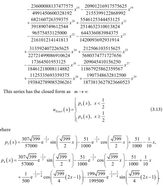
This series has the closed form as m→ ∞
( )
( )
( )
3
4
1 ,
2 1 ,
2
Exact
p x x
u x
p x x
<
=
≥
(3.13)
where
( )
12 123 307 39957000 e sin 3992 100051 e cos 3992 1000 1051 1 ,
x x
p x = − x− − x+ − x
( )
(
)
(
)
1 1
2 2
4
1 1 1 1
2 4 2 4
307 399e sin 399 51 e cos 399 51 1
57000 2 1000 2 1000 10
1 e cos 399 2 1 199 399e sin 399 2 1 ,
500 4 199500 4
x x
x x
p x x x x
x x
− −
− + − +
= − − +
+ − − −
which is exactly the exact solution for the case 3.1.1.
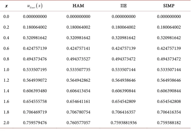
In Table 1 show a comparison of the numerical results applying the HAM (m=15), Iteration of the Integral Equation (IIE) (3.9), and the numerical solu-tion of (3.9) with Simpson rule (SIMP) with the exact solusolu-tion (3.13). Twenty points have been used in the Simpson rule. In Table 2 we list the Maximum Absolute Error (MAE), ⋅ 2, the Maximum Relative Error (MRE), the
[image:6.595.210.540.66.441.2]Maxi-mum Residual Error (MRR), obtained by the HAM with the exact solution (3.13) on the interval
[ ]
0,1 . The Estimated Order of Convergence (EOC) for different values of the constant k are given in Table 3.Figure 1 represents both the exact solution uExact
( )
x and our approximation by HAM (m=14) within the interval 0≤ ≤t 1.For k≥13, the application of the HAM requires approximants of order 15
m> if we want to arrive beyond the discontinuity (at 1
2
x= ).
Case 3.1.2 Taking β =1,k=1,λ=1 and
(
, ,)
(
1)
0, if 11, if 1,
x
f x u u H x
x
<
′ = − =
≥
(3.14)
DOI: 10.4236/am.2019.106030 425 Applied Mathematics
[image:7.595.291.459.69.213.2]Figure 1. Continuous line: uExact
( )
x , : HAM,+ λ=10,k=10.Table 1. Numerical results for the case 3.1.1.
x uExact
( )
x HAM IIE SIMP [image:7.595.210.540.265.486.2]0.0 0.000000000 0.000000000 0.000000000 0.000000000 0.1 0.100782334 0.100782334 0.100782334 0.100782334 0.2 0.138716799 0.138716799 0.138716799 0.138716799 0.3 0.077844715 0.077844715 0.077844715 0.077844715 0.4 −0.027921565 −0.027921565 −0.027921565 −0.027921565 0.5 −0.090520718 −0.090520718 −0.090520718 −0.090520718 0.6 −0.064945725 −0.064945725 −0.064945723 −0.064945723 0.7 0.023844667 0.023844566 0.023844678 0.023844678 0.8 0.100898402 0.100896153 0.100898714 0.100898714 0.9 0.108664846 0.108638517 0.108670237 0.108670234 1.0 0.055691769 0.055659061 0.055736683 0.055736417
Table 2. MAE, ⋅2, MRE and MRR for the case 3.1.1.
m MAE ⋅2 MRE MRR
12 1.104E−01 1.474E−02 1.983E−00 89.418E−00 13 1.541E−02 1.889E−03 2.767E−01 16.061E−00 14 1.360E−03 1.408E−04 2.443E−02 2.222E−00 15 6.803E−05 1.732E−05 9.487E−04 1.940E−01
Table 3. EOC for the case 3.1.1.
k x=0.4 x=0.6
10 1.0660 1.0778
11 1.0628 1.0824
[image:7.595.209.541.525.614.2]DOI: 10.4236/am.2019.106030 426 Applied Mathematics
( )
0 ,
u x =x
( )
3 2
1
3
1 1 , 1 6 2 , 1 1 , 1
6 2
hx hx x
u x
hx hx h x
+ <
=
+ − ≥
( )
(
)
2 5 2 4 3 2
2
2 5 2 4 3
1 1 1 1 1 1 , 1
120 12 3 2 2
, 1 1 1 1 2 1 1 1 3 , 1 120 24 3 2 3 2 4
h x h x hx h hx h x
u x
h x h x hx h hx h h h x
+ + + + + <
= + + + + + − + ≥
and so on, in this manner the rest of the iterations can be obtained. Thus, the approximate solution in a series form when h= −1 is
( )
( )
( )
( )
( )
9 5 0 1 6 , 1 , 1 m mp x x
u x u x u x
p x x
= < = + = ≥
∑
(3.15)where
( )
2 4 5 7 8 105
11 12 13 14
15 16 17
1 1 1 1 1 1
2 24 120 5040 40320 1814400
1 1 1 1
5702400 17740800 124540416 1779148800
1 1 1
48432384000 2615348736000 355687428096000
p x x x x x x x x
x x x x
x x x
= − + − + − +
+ + + +
+ + +
and
( )
26
3 4 5
6 7 8
4581894569957 294371651437 23051120003 6974263296000 653837184000 58118860800
355931929 215859517 251909 6227020800 11496038400 38016000
422017 80707 11293 870912000 914457600 541900800
p x x x
x x x
x x x
= − +
− − +
− − +
9 10 11
12 13 14
15 16 17
463 401 211 304819200 2612736000 798336000
19 113 71
348364800 18681062400 174356582400
1 1 1
62270208000 2988969984000 355687428096000
x x x
x x x
x x x
− + +
+ + +
+ + +
This series has the closed form as m→ ∞
( )
(
)
(
)
1 2
1 1 1
2 2 2
1 1 2 2
2 3e sin 1 3 , 1
3 2
2 3e sin 3 3e sin 3 1
3 2 3 2
3
e cos 1 1, 1, 2 x x x Exact x x x
u x x x
x x
−
− − +
− +
<
DOI: 10.4236/am.2019.106030 427 Applied Mathematics which is exactly the exact solution for the case 3.1.2.
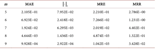
In Table 4 show a comparison of the numerical results applying the HAM (m=9), Iteration of the Integral Equation (IIE) (3.9), and the numerical solu-tion of (3.9) with Simpson rule (SIMP) with the exact solusolu-tion (3.16). In Table 5 we list the MAE, ⋅ 2, the MRE, and the MRR, obtained by the HAM with
[image:9.595.290.458.263.452.2]the exact solution (3.16) on the interval
[ ]
0,1 . The EOC for different values of the constant k are given in Table 6.Figure 2 represents both the exact solution uExact
( )
x and our approximation by HAM (m=9) within the interval 0≤ ≤t 2.Case 3.1.3 Taking β =1,k=1,λ=1 and
(
, ,)
(
1)
f x u u′ =
δ
x− , the Dirac delta function at x=1. We now successively obtain( )
0 ,
u x =x
[image:9.595.211.541.503.727.2]Figure 2. Continuous line: uExact
( )
x , : HAM,+ λ=1,? 1k= .Table 4. Numerical results for the case 3.1.2.
x uExact
( )
x HAM IIE SIMPDOI: 10.4236/am.2019.106030 428 Applied Mathematics
Table 5. MAE, ⋅2, MRE and MRR for the case 3.1.2.
m MAE ⋅2 MRE MRR
5 2.214E−01 8.262E−02 2.914E−01 3.091E−00 6 7.122E−02 2.471E−02 9.377E−02 1.313E−00 7 1.955E−02 6.370E−03 2.573E−02 4.573E−01 8 4.684E−03 1.446E−03 6.167E−03 1.351E−01 9 9.976E−04 2.933E−04 1.313E−03 3.471E−02
Table 6. EOC for the case 3.1.2.
k x=0.9 x=1.1
1 1.0871 1.1001
2 1.1081 1.1300
( )
(
3 2(
)
(
)
)
1 16 3 6 1 6 1
u x = − h x− − x + H x− x− H x−
( )
(
(
)
(
)
(
)
(
) (
)
(
)(
)
)
5 4 3 3
2
2
1 10 20 2 1 20 1 120
60 1 60 1 2 40 1 2 3
u x h hx hx x h hH x x
x h H x x h H x h
= − − − − + + −
− + + − + − − +
and so on, in this manner the rest of the iterations can be obtained. Thus, the approximate solution in a series form when h= −1 is
( )
( )
( )
(
)
8 0
1
2
3 4 5 6
7 8 9 10
9030495007 858929737 2734477 1
6227020800 479001600 15966720 5271359 653741 14383 7477 21772800 8709120 4838400 3628800
293 71 71 23 725760 4838400 8709120 21772800
17 79
m m
u x u x u x
H x x x
x x x x
x x x x
=
= +
= − − + −
− + − −
+ − − +
+
∑
11 1 12 1 13
833600x +95800320x +6227020800x
2 4 5 7 8 9
10 11 12 13
14 15
1 1 1 1 1 1
2 24 120 5040 40320 362880
1 1 29 1
604800 1900800 479001600 311351040
1 1
12454041600 1307674368000
x x x x x x x
x x x x
x x
− + − + − −
− − − −
− −
+
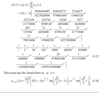
(3.17)
This series has the closed form as m→ ∞
( )
2 3(
1 e)
1 12 2 sin 3(
1)
e 21 sin 33 2 2
x x
Exact
u x = H x− − x− + − x
[image:10.595.205.537.426.740.2]DOI: 10.4236/am.2019.106030 429 Applied Mathematics which is exactly the exact solution for the case 3.1.3.
In Table 7 we list the MAE, ⋅ 2, the MRE, and the MRR, obtained by the
HAM with the exact solution (3.18) on the interval
[ ]
0,2 . The EOC are 1.0984 at x=0.9 and 1.1156 at x=1.1.Figure 3 gives both the exact solution uExact
( )
x and our approximation by HAM (m=8) within the interval 0≤ ≤t 2.3.2. Non-Linear Case
Let
α
=0,β
=1,λ
=10 and k=1.Case 3.2.1 Taking g u u
(
, ′)
=uu′, and(
)
1 0, if
2 , ,
1 1, if
2
x f x u u
x
<
′ =
≥
(3.19)
Using the Adomian polynomials [8] [9] for calculation the nonlinear term uu′ is given by
(
)
0
, n i n i, , 0,1,2,
i
g u u uu u u − n i n
=
′ = ′=
∑
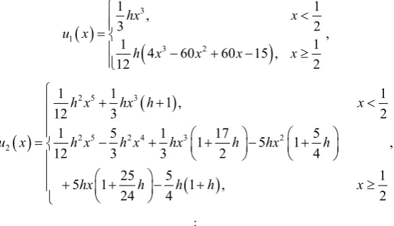
′ ≥ = (3.20)We now successively obtain
( )
0 ,
[image:11.595.282.466.332.568.2]u x =x
[image:11.595.210.541.621.726.2]Figure 3. Continuous line: uExact
( )
x , : HAM,+ λ=1,k=1.Table 7. MAE, ⋅2, MRE and MRR for the case 3.1.3.
m MAE ⋅2 MRE MRR
DOI: 10.4236/am.2019.106030 430 Applied Mathematics
( )
(
)
3 1 3 21 , 1
3 2 ,
1 4 60 60 15 , 1
12 2
hx x
u x
h x x x x
< = − + − ≥
( )
(
)
(
)
2 5 3
2 5 2 4 3 2
2
1 1 1 , 1
12 3 2
1 5 1 1 17 5 1 5 ,
12 3 3 2 4
25 5 1
5 1 1 ,
24 4 2
h x hx h x
u x h x h x hx h hx h
hx h h h x
+ + <
= − + + − + + + − + ≥
and so on, in this manner the rest of the iterations can be obtained. Thus, the approximate solution in a series form when h= −1 is
( )
( )
( )
( )
( )
7 7 0 1 8 1 , 2 , 1 , 2 m mp x x
u x u x u x
p x x
= < = + = ≥
∑
(3.21)where
( )
3 5 7 9 11 137 13 121 50411 36288211 39916806221 622702080260833
p x = −x x + x − x + x − x + x
and
( )
2 38
4 5 6 7
8 9 10
131015952083 846993899 1362271259 202153183 98099527680 181665792 185794560 37158912
44111605 37786871 156205 4167853 6193152 7741440 165888 645120 18511 431939 3502817
2016 64512 1451520
p x x x x
x x x x
x x x
= − + −
+ − − +
− + − 11
12 13 267623 725760 520067 260833 23950080 622702080 x x x + − +
In Table 8 show a comparison of the numerical results applying the HAM (m=7), Iteration of the Integral Equation (IIE) (3.9), and the numerical solu-tion of (3.9) with Simpson rule (SIMP) with the numeric solusolu-tion (rkf45)
( )
Nu x . In Table 9 we list the MAE, the MRE, and the MRR, obtained by the HAM with the numeric solution (rkf45) u xN
( )
on the interval[ ]
0,1 .Figure 4 represents both the numeric solution (rkf45) u xN
( )
with a very small error and our approximation by HAM (m=7) within the interval0≤ ≤t 1.
Case 3.2.2 Taking g u u
(
, ′ =)
u2, and(
, ,)
0, if 11, if 1
x f x u u
x
<
′ =
≥
(3.22)
Using the Adomian polynomials [8] [9] for calculation the nonlinear term u2
[image:12.595.235.512.74.233.2]DOI: 10.4236/am.2019.106030 431 Applied Mathematics
[image:13.595.211.541.294.538.2]Figure 4. Continuous line: u xN
( )
, : HAM,+ λ=10,k=1.Table 8. Numerical results for the case 3.2.1.
x rkf45 HAM IIE SIMP
0.0 0.000000000 0.000000000 0.000000000 0.000000000
0.1 0.099667499 0.099667497 0.099667497 0.099667497
0.2 0.197359727 0.197359723 0.197359723 0.197359723
0.3 0.291197840 0.291197838 0.291197838 0.291197838
0.4 0.379485700 0.379485702 0.379485702 0.379485702
0.5 0.460777633 0.460777635 0.460777632 0.460777632
0.6 0.583008128 0.583008017 0.583007978 0.583007978
0.7 0.789366837 0.789366701 0.789366561 0.789366561
0.8 1.068091674 1.068091572 1.068091282 1.068091282
0.9 1.402735913 1.402734083 1.402735383 1.402735385
1.0 1.773297313 1.773238159 1.773299771 1.773299790
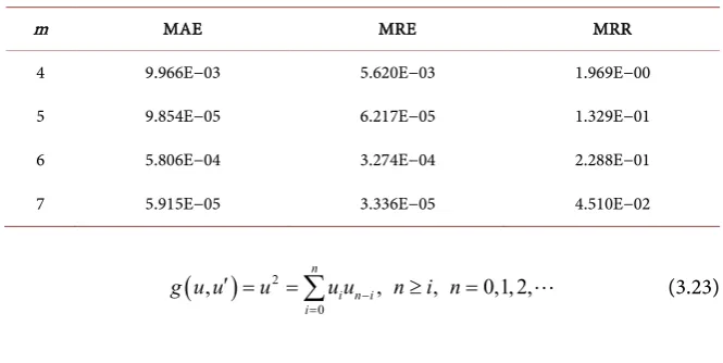
Table 9. MAE, MRE and MRR for the case 3.2.1.
m MAE MRE MRR
4 9.966E−03 5.620E−03 1.969E−00
5 9.854E−05 6.217E−05 1.329E−01
6 5.806E−04 3.274E−04 2.288E−01
7 5.915E−05 3.336E−05 4.510E−02
(
)
20
, n i n i, , 0,1,2,
i
g u u u u u − n i n
=
[image:13.595.207.540.570.737.2]DOI: 10.4236/am.2019.106030 432 Applied Mathematics we now successively obtain
( )
0 ,
u x =x
( )
(
4 3)
(
)
(
2)
1 121 2 5 1 2 1 ,
u x = h x + x − hH x− x − x+
( )
(
)
(
)
(
)
5 4 2
2
2 7 6
5 4 3 4 3
1 1 1260 3150 18900 31500 2520
1
12600 14490 25200 12600 10 35 2520
21 210 420 210 420 ,
u x hH x hx hx hx hx
x h x h hx hx
hx hx hx x x
= − − − + −
+ + − + + +
+ + + + +
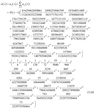
and so on, in this manner the rest of the iterations can be obtained. Thus, the approximate solution in a series form when h= −1 is
( )
( )
( )
(
)
8 0 1 23 4 5 6
41629462050061 2498253046769 18764031409 1
11263435223040 563171761152 4704860160 1761739129 502232959 1677121153 10243801115
274450176 181621440 242161920 581188608 341190523
m m
u x u x u x
H x x x
x x x x
= = + = − − − + − + − +
∑
7 8 9 10
11 12 13 14
150931763 11334138401 2673838147 13453440 6209280 670602240 304819200 2650717003 1572737 88586453 213052381 79833600 1905120 1089728640 8717829120
x x x x
x x x x
− + −
+ − + +
15 16 17
18 19 20
3 4 5 6 7 8
9 10
6247867 71250341 48109
605404800 58118860800 823350528
1322521 74645 157891
59281238016 140792940288 1126343522304
1 1 1 1 19 1
6 12 120 72 5040 960
299 43
362880 362880
x x x
x x x
x x x x x x x
x x − + + − + + − − + + + − − − +
+ 3239 11 869 12
39916800x +21772800x
13 14 15
16 17 18
19 20 21
22
8201 53 2150341
6227020800 10644480 1307674368000
1660739 20675 11819
10461394944000 79041650688 209227898880
12799 743 803
750895681536 56458321920 252975550464
73 252975550464
x x x
x x x
x x x
x + − − + + + − − − − (3.24)
In Table 10 we list the MAE, the MRE, and the MRR, obtained by the HAM with the numeric solution (rkf45) u xN
( )
on the interval[ ]
0,2 .Figure 5 represents both the numeric solution (rkf45) u xN
( )
with a very small error and our approximation by HAM (m=8) within the interval [image:14.595.215.538.271.640.2]DOI: 10.4236/am.2019.106030 433 Applied Mathematics
Figure 5. Continuous line: u xN
( )
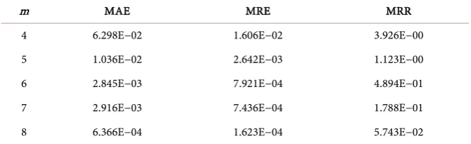
, : HAM,+ λ=10,k=1.Table 10. MAE, MRE and MRR for the case 3.2.2.
m MAE MRE MRR
4 6.298E−02 1.606E−02 3.926E−00
5 1.036E−02 2.642E−03 1.123E−00
6 2.845E−03 7.921E−04 4.894E−01
7 2.916E−03 7.436E−04 1.788E−01
8 6.366E−04 1.623E−04 5.743E−02
4. Conclusions
In this work, the HAM has been successfully applied to solve IVPs of second or-der with discontinuities. The size of the jump (given by λ) does not affect the convergence of the method, which behaves equally well on both sides of the dis-continuity. In this IVPs, the application by the HAM with k, does not converge even for small values of the parameter like λ.
The proposed scheme of the HAM has been applied directly without any need for transformation formulae or restrictive assumptions. The solution process by the HAM is compatible with the method in the literature providing analytical approximation such as ADM. The approach of the HAM has been tested by em-ploying the method to obtain approximate-exact solutions of the linear case. The results obtained in all cases demonstrate the reliability and the efficiency of this method.
Conflicts of Interest
The authors declare no conflicts of interest regarding the publication of this pa-per.
References
[image:15.595.209.540.295.396.2]Uni-DOI: 10.4236/am.2019.106030 434 Applied Mathematics versity, Shanghai.
[2] Liao, S.J. (1999) An Explicit, Totally Analytic Approximation of Blasius' Viscous Flow Problems. International Journal of Non-Linear Mechanics, 34, 759-778.
https://doi.org/10.1016/s0020-7462(98)00056-0
[3] Liao, S.J. (2003) Beyond Perturbation: Introduction to the Homotopy Analysis Me-thod. CRC Press, Boca Raton.
[4] Casasús, L. and Al-Hayani, W. (2002) The Decomposition Method for Ordinary Differential Equations with Discontinuities. Applied Mathematics and Computa-tion, 131, 245-251.https://doi.org/10.1016/s0096-3003(01)00142-4
[5] Al-Hayani, W. and Casasús, L. (2006) On the Applicability of the Adomian Method to Initial Value Problems with Discontinuities. Applied Mathematics Letters, 19, 22-31. https://doi.org/10.1016/j.aml.2005.03.004
[6] He, J.-H. (2004) The Homotopy Perturbation Method for Nonlinear Oscillators with Discontinuities. Applied Mathematics and Computation, 151, 287-292.
https://doi.org/10.1016/s0096-3003(03)00341-2
[7] He, J.-H. (2003) Homotopy Perturbation Method: A New Nonlinear Analytical Technique. Applied Mathematics and Computation, 135, 73-79.
https://doi.org/10.1016/s0096-3003(01)00312-5
[8] Adomian, G. (1986) Nonlinear Stochastic Operator Equations. Academic Press, New York.
[9] Wazwaz, A.M. (2000) A New Algorithm for Calculating Adomian Polynomials for Nonlinear Operators. Applied Mathematics and Computation, 111, 53-69.