Space Telescope and Optical Reverberation Mapping Project. VIII. Time Variability of
Emission and Absorption in NGC 5548 Based on Modeling the Ultraviolet Spectrum
G. A. Kriss1 , G. De Rosa1 , J. Ely1 , B. M. Peterson1,2,3 , J. Kaastra4,5, M. Mehdipour4, G. J. Ferland6 , M. Dehghanian6 , S. Mathur2,3, R. Edelson7 , K. T. Korista8 , N. Arav9, A. J. Barth10 , M. C. Bentz11 , W. N. Brandt12,13,14 , D. M. Crenshaw11 , E. Dalla Bontà15,16, K. D. Denney2,3,17, C. Done18, M. Eracleous12,13 , M. M. Fausnaugh2,19 , E. Gardner20, M. R. Goad21 , C. J. Grier2,22 , Keith Horne23 , C. S. Kochanek2,3 , I. M. McHardy24, H. Netzer25 , A. Pancoast26,107 , L. Pei10, R. W. Pogge2,3 , D. Proga27 , C. Silva4,28, N. Tejos29, M. Vestergaard22,30 , S. M. Adams2,31, M. D. Anderson11, P. Arévalo32, T G. Beatty2,12,33 , E. Behar34, V. N. Bennert35 , S. Bianchi36, A. Bigley37, S. Bisogni2,26,38 , R. Boissay-Malaquin39 , G. A. Borman40, M. C. Bottorff41, A. A. Breeveld42 , M. Brotherton43, J. E. Brown44, J. S. Brown2,45, E. M. Cackett46 , G. Canalizo47, M. Cappi48, M. T. Carini49, K. I. Clubb37, J. M. Comerford50, C. T. Coker2 , E. M. Corsini15,16,
E. Costantini4 , S. Croft37 , K. V. Croxall2,3,51 , A. J. Deason45,52 , A. De Lorenzo-Cáceres23,53, B. De Marco54, M. Dietrich51,108, L. Di Gesu55, J. Ebrero56, P. A. Evans7, A. V. Filippenko57,58,109 , K. Flatland59,60, E. L. Gates61, N. Gehrels62,110, S. Geier53,63,64, J. M. Gelbord65,66, L. Gonzalez59, V. Gorjian67, D. Grupe68 , A. Gupta2, P. B. Hall69 ,
C. B. Henderson2,67,111 , S. Hicks49, E. Holmbeck70 , T. W.-S. Holoien2,3,71 , T. A. Hutchison41,72,73 , M. Im74 , J. J. Jensen75, C. A. Johnson76, M. D. Joner77, S. Kaspi25,34, B. C. Kelly78, P. L. Kelly79,80,81 , J. A. Kennea12 , M. Kim82, S. C. Kim83, S. Y. Kim2,3, A. King84, S. A. Klimanov85, Y. Krongold86, M. W. Lau45,47, J. C. Lee83, D. C. Leonard59, Miao Li87,
P. Lira88, C. Lochhaas2, Zhiyuan Ma41 , F. MacInnis41, M. A. Malkan70 , E. R. Manne-Nicholas11, G. Matt36 , J. C. Mauerhan37 , R. McGurk45,71, C. Montuori89, L. Morelli15,16,90, A. Mosquera2,91, D. Mudd2,10, F. Müller-Sánchez50,92, S. V. Nazarov40, R. P. Norris11, J. A. Nousek12, M. L. Nguyen43, P. Ochner15,16, D. N. Okhmat40, S. Paltani93, J. R. Parks11, C. Pinto94, A. Pizzella15,16, R. Poleski2, G. Ponti95, J.-U. Pott96, S. E. Rafter34,97, H.-W. Rix96 , J. Runnoe98, D. A. Saylor11, J. S. Schimoia2,99, K. Schnülle96, B. Scott47, S. G. Sergeev40, B. J. Shappee2,100 , I. Shivvers37, M. Siegel101, G. V. Simonian2, A. Siviero15, A. Skielboe75, G. Somers2,102, M. Spencer77, D. Starkey23,103, D. J. Stevens2,12,33, H.-I. Sung83, J. Tayar2,100,112 ,
K. G. Teems11, T. Treu70,113, C. S. Turner11, P. Uttley28, J . Van Saders2,100, L. Vican70, C. Villforth104, S. Villanueva Jr.2, D. J. Walton94 , T. Waters105, Y. Weiss34, J.-H. Woo74, H. Yan44, H. Yuk37, W. Zheng37, W. Zhu2, and Y. Zu2,106
1
Space Telescope Science Institute, 3700 San Martin Drive, Baltimore, MD 21218, USA
2
Department of Astronomy, The Ohio State University, 140 West 18th Avenue, Columbus, OH 43210, USA
3
Center for Cosmology and AstroParticle Physics, The Ohio State University, 191 West Woodruff Avenue, Columbus, OH 43210, USA
4
SRON Netherlands Institute for Space Research, Sorbonnelaan 2, 3584 CA Utrecht, The Netherlands
5
Leiden Observatory, Leiden University, P.O. Box 9513, 2300 RA Leiden, The Netherlands
6Department of Physics and Astronomy, The University of Kentucky, Lexington, KY 40506, USA 7
Department of Astronomy, University of Maryland, College Park, MD 20742, USA
8
Department of Physics, Western Michigan University, 1120 Everett Tower, Kalamazoo, MI 49008, USA
9
Department of Physics, Virginia Tech, Blacksburg, VA 24061, USA
10
Department of Physics and Astronomy, 4129 Frederick Reines Hall, University of California, Irvine, CA 92697, USA
11
Department of Physics and Astronomy, Georgia State University, 25 Park Place, Suite 605, Atlanta, GA 30303, USA
12
Department of Astronomy and Astrophysics, Eberly College of Science, The Pennsylvania State University, 525 Davey Laboratory, University Park, PA 16802, USA
13
Institute for Gravitation and the Cosmos, The Pennsylvania State University, University Park, PA 16802, USA
14
Department of Physics, 104 Davey Lab, The Pennsylvania State University, University Park, PA 16802, USA
15Dipartimento di Fisica e Astronomia“G. Galilei,”Università di Padova, Vicolo dell’Osservatorio 3, I-35122 Padova, Italy 16
INAF–Osservatorio Astronomico di Padova, Vicolo dell’Osservatorio 5 I-35122, Padova, Italy
17
Illumination Works, LLC, 5650 Blazer Parkway, Dublin, OH 43017, USA
18
Centre for Extragalactic Astronomy, Department of Physics, University of Durham, South Road, Durham DH1 3LE, UK
19
Department of Physics, Massachusetts Institute of Technology, 77 Massachusetts Avenue, Cambridge, MA 02139-4307, USA
20
School of Biological Sciences, University of Reading, Whiteknights, Reading, RG6 6AS, UK
21
Department of Physics and Astronomy, University of Leicester, Leicester, LE1 7RH, UK
22
Steward Observatory, University of Arizona, 933 North Cherry Avenue, Tucson, AZ 85721, USA
23
SUPA Physics and Astronomy, University of St. Andrews, Fife, KY16 9SS Scotland, UK
24
University of Southampton, Highfield, Southampton, SO17 1BJ, UK
25
School of Physics and Astronomy, Raymond and Beverly Sackler Faculty of Exact Sciences, Tel Aviv University, Tel Aviv 69978, Israel
26Harvard-Smithsonian Center for Astrophysics, 60 Garden Street, Cambridge, MA 02138, USA 27
Department of Physics & Astronomy, University of Nevada, Las Vegas, 4505 South Maryland Parkway, Box 454002, Las Vegas, NV 89154-4002, USA
28
Astronomical Institute“Anton Pannekoek,”University of Amsterdam, Science Park 904, 1098 XH Amsterdam, The Netherlands
29
Instituto de Física, Pontificia Universidad Católica de Valparaíso, Casilla 4059, Valparaíso, Chile
30
DARK, Niels Bohr Institute, University of Copenhagen, Lyngbyvej 2, DK-2100 Copenhagen Ø, Denmark
31
Cahill Center for Astrophysics, California Institute of Technology, Pasadena, CA 91125, USA
32
Instituto de Física y Astronomía, Facultad de Ciencias, Universidad de Valparaíso, Gran Bretana N 1111, Playa Ancha, Valparaíso, Chile
33
Center for Exoplanets and Habitable Worlds, The Pennsylvania State University, University Park, PA 16802, USA
34
Department of Physics, Technion-Israel Institute of Technology, 32000 Haifa, Israel
35Physics Department, California Polytechnic State University, San Luis Obispo, CA 93407, USA 36
Dipartimento di Matematica e Fisica, Università degli Studi Roma Tre, via della Vasca Navale 84, I-00146 Roma, Italy
37Department of Astronomy, University of California, Berkeley, CA 94720, USA 38
Osservatorio Astrofisico di Arcetri, largo E. Fermi 5, I-50125, Firenze, Italy
39
Kavli Institute for Astrophysics and Space Research, Massachusetts Institute of Technology, 77 Massachusetts Avenue, Cambridge, MA 02139, USA
40
Crimean Astrophysical Observatory, P/O Nauchny, Crimea 298409, Russia
41
Fountainwood Observatory, Department of Physics FJS 149, Southwestern University, 1011 East University Avenue, Georgetown, TX 78626, USA
42Mullard Space Science Laboratory, University College London, Holmbury St. Mary, Dorking, Surrey RH5 6NT, UK 43
Department of Physics and Astronomy, University of Wyoming, 1000 East University Avenue, Laramie, WY 82071, USA
44
Department of Physics and Astronomy, University of Missouri, Columbia, MO 65211, USA
45
Department of Astronomy and Astrophysics, University of California Santa Cruz, 1156 High Street, Santa Cruz, CA 95064, USA
46
Department of Physics and Astronomy, Wayne State University, 666 West Hancock Street, Detroit, MI 48201, USA
47
Department of Astronomy, University of California, Riverside, CA 92521, USA
48
INAF-IASF Bologna, Via Gobetti 101, I-40129 Bologna, Italy
49
Department of Physics and Astronomy, Western Kentucky University, 1906 College Heights Boulevard#11077, Bowling Green, KY 42101, USA
50
Department of Astrophysical and Planetary Sciences, University of Colorado, Boulder, CO 80309, USA
51Department of Earth, Environment and Physics, Worcester State University, Worcester, MA 01602, USA 52
Institute for Computational Cosmology, Department of Physics, University of Durham, South Road, Durham DH1 3LE, UK
53
Instituto de Astrofísica de Canarias, E-38200 La Laguna, Tenerife, Spain
54
Nicolaus Copernicus Astronomical Center, Polish Academy of Sciences, Bartycka 18, PL-00-716 Warsaw, Poland
55
Italian Space Agency(ASI), Via del Politecnico snc I-00133 Rome, Italy
56
European Space Astronomy Centre, P.O. Box 78, E-28691 Villanueva de la Cañada, Madrid, Spain
57
Department of Astronomy, University of California, Berkeley, CA 94720-3411, USA
58
Miller Institute for Basic Research in Science, University of California, Berkeley, CA 94720, USA
59
Department of Astronomy, San Diego State University, San Diego, CA 92182, USA
60
Oakwood School, 105 John Wilson Way, Morgan Hill, CA 95037, USA
61
Lick Observatory, P.O. Box 85, Mt. Hamilton, CA 95140, USA
62
Astrophysics Science Division, NASA Goddard Space Flight Center, Mail Code 661, Greenbelt, MD 20771, USA
63
Departamento de Astrofísica, Universidad de La Laguna, E-38206 La Laguna, Tenerife, Spain
64
Gran Telescopio Canarias(GRANTECAN), E-38205 San Cristóbal de La Laguna, Tenerife, Spain
65
Spectral Sciences Inc., 4 Fourth Avenue, Burlington, MA 01803, USA
66
Eureka Scientific Inc., 2452 Delmer Street Suite 100, Oakland, CA 94602, USA
67
Jet Propulsion Laboratory, California Institute of Technology, 4800 Oak Grove Drive, Pasadena, CA 91109, USA
68
Space Science Center, Morehead State University, 235 Martindale Drive, Morehead, KY 40351, USA
69
Department of Physics and Astronomy, York University, Toronto, ON M3J 1P3, Canada
70
Department of Physics and Astronomy, University of California, Los Angeles, CA 90095, USA
71
The Observatories of the Carnegie Institution for Science, 813 Santa Barbara Street, Pasadena, CA 91101, USA
72
Department of Physics and Astronomy, Texas A&M University, College Station, TX 77843-4242 USA
73
George P. and Cynthia Woods Mitchell Institute for Fundamental Physics and Astronomy, Texas A&M University, College Station, TX 77843-4242, USA
74
Astronomy Program, Department of Physics & Astronomy, Seoul National University, Seoul, Republic of Korea
75
Dark Cosmology Centre, Niels Bohr Institute, University of Copenhagen, Juliane Maries Vej 30, DK-2100 Copenhagen Ø, Denmark
76
Santa Cruz Institute for Particle Physics and Department of Physics, University of California, Santa Cruz, CA 95064, USA
77
Department of Physics and Astronomy, N283 ESC, Brigham Young University, Provo, UT 84602, USA
78
Department of Physics, University of California, Santa Barbara, CA 93106, USA
79
Department of Physics, Stanford University, 382 Via Pueblo Mall, Stanford, CA 94305, USA
80Kavli Institute for Particle Astrophysics and Cosmology, Stanford University, Stanford, CA 94305, USA 81
SLAC National Accelerator Laboratory, 2575 Sand Hill Road, Menlo Park, CA 94025, USA
82
Department of Astronomy and Atmospheric Sciences, Kyungpook National University, Daegu 702-701, Republic of Korea
83
Korea Astronomy and Space Science Institute, Daejeon 34055, Republic of Korea
84
School of Physics, University of Melbourne, Parkville, VIC 3010, Australia
85
Pulkovo Observatory, 196140 St. Petersburg, Russia
86
Instituto de Astronomía, Universidad Nacional Autonoma de Mexico, Cuidad de Mexico, Mexico
87
Department of Astronomy, Columbia University, 550 West 120th Street, New York, NY 10027, USA
88
Departamento de Astronomia, Universidad de Chile, Camino del Observatorio 1515, Santiago, Chile
89DiSAT, Universita dell’Insubria, via Valleggio 11, I-22100, Como, Italy 90
Instituto de Astronomia y Ciencias Planetarias, Universidad de Atacama, Copiapó, Chile
91
Physics Department, United States Naval Academy, Annapolis, MD 21403, USA
92
Department of Physics and Materials Science, The University of Memphis, 3720 Alumni Avenue, Memphis, TN 38152, USA
93
Department of Astronomy, University of Geneva, 16 Ch. d’Ecogia, 1290 Versoix, Switzerland
94
Institute of Astronomy, Madingley Road, CB3 0HA Cambridge, UK
95
INAF–Osservatorio Astronomico di Brera, Via E. Bianchi 46, I-23807 Merate(LC), Italy
96
Max Planck Institut für Astronomie, Königstuhl 17, D-69117 Heidelberg, Germany
97
Department of Physics, Faculty of Natural Sciences, University of Haifa, Haifa 31905, Israel
98
Department of Astronomy, University of Michigan, 1085 South University Avenue, Ann Arbor, MI 48109, USA
99
Laboratório Interinstitucional de e-Astronomia, Rua General José Cristino, 77 Vasco da Gama, Rio de Janeiro, RJ, Brazil
100Institute for Astronomy, 2680 Woodlawn Drive, Honolulu, HI 96822-1839, USA 101
Las Cumbres Observatory Global Telescope Network, 6740 Cortona Drive, Suite 102, Goleta, CA 93117, USA
102
Department of Physics and Astronomy, Vanderbilt University, 6301 Stevenson Circle, Nashville, TN 37235, USA
103
Department of Astronomy, University of Illinois Urbana-Champaign, 1002 West Green Street, Urbana, IL 61801, USA
104
105
Applied Physics Division, Los Alamos National Laboratory, Los Alamos, NM 87545, USA
106Shanghai Jiao Tong University, 800 Dongchuan Road, Shanghai, 200240, People’s Republic of China
Received 2019 March 29; revised 2019 June 27; accepted 2019 July 6; published 2019 August 22
Abstract
We model the ultraviolet spectra of the Seyfert 1 galaxy NGC5548 obtained with theHubble Space Telescope during the 6 month reverberation mapping campaign in 2014. Our model of the emission from NGC 5548 corrects for overlying absorption and deblends the individual emission lines. Using the modeled spectra, we measure the response to continuum variations for the deblended and absorption-corrected individual broad emission lines, the velocity-dependent profiles of Lyαand CIV, and the narrow and broad intrinsic absorption features. Wefind that the time lags for the corrected emission lines are comparable to those for the original data. The velocity-binned lag profiles of Lyα and CIV have a double-peaked structure indicative of a truncated Keplerian disk. The narrow absorption lines show a delayed response to continuum variations corresponding to recombination in gas with a density of ∼105cm−3. The high-ionization narrow absorption lines decorrelate from continuum variations during the same period as the broad emission lines. Analyzing the response of these absorption lines during this period shows that the ionizing flux is diminished in strength relative to the far-ultraviolet continuum. The broad absorption lines associated with the X-ray obscurer decrease in strength during this same time interval. The appearance of X-ray obscuration in∼2012 corresponds with an increase in the luminosity of NGC 5548 following an extended low state. We suggest that the obscurer is a disk wind triggered by the brightening of NGC 5548 following the decrease in size of the broad-line region during the preceding low-luminosity state.
Key words:galaxies: active–galaxies: individual(NGC 5548)–galaxies: nuclei–galaxies: Seyfert Supporting material:machine-readable tables
1. Introduction
Quantitatively measuring the geometry, kinematics, and physical conditions in the structures at the centers of active galactic nuclei(AGNs)is essential for understanding how their activity is fueled by inflowing gas and how outflows from the central engine may influence the surrounding host galaxy. Even in the nearest AGN, the broad-line region (BLR) and the accretion disk are nearly impossible to resolve at optical, ultraviolet (UV), or X-ray wavelengths, although the Gravity Collaboration et al. (2018) used near-IR interferometry to detect the spatial extent of the BLR of the quasar 3C 273 at an angular size of∼10μas. Reverberation mapping(Blandford & McKee 1982; Peterson 1993) provides a powerful technique for resolving features on physical scales 10 times smaller. A resolution of light-days, corresponding to angular scales of microarcseconds, suffices to probe the detailed structure of the BLR and accretion disks of nearby AGNs.
The Seyfert galaxy NGC 5548 has been a prime target of several successful reverberation mapping campaigns, both in the UV from space(Clavel et al.1991; Korista et al.1995)and in the optical from the ground (see Peterson et al. 2002, and references therein). These campaigns ascertained that the typical size of the BLR is several light-days and established
that it was likely dominated by virial motions, since the size, ionization stratification, and line widths are all consistent with motions in a gravitational field (Peterson & Wandel 1999). These initial campaigns measured only the mean lag and line width for selected emission lines. Spurred by these successes and the promise of higher-quality data, more recent campaigns have explored the possibility of measuring lags in two dimensions with velocity-resolved reverberation mapping across strong emission-line profiles(Horne et al. 2004; Bentz et al.2010; Grier et al.2013).
Early efforts at velocity-resolved reverberation mapping from the ground were followed in 2014 by thefirst attempt to determine high-quality velocity-resolved delay maps for NGC 5548 by the AGN Space Telescope and Optical Reverberation Mapping program(AGN STORM; PI: Peterson; De Rosa et al.
2015). This program monitored NGC 5548 on a nearly daily basis for approximately 6 months using the Hubble Space Telescope (HST), the Neil Gehrels Swift Observatory, and several ground-based facilities, producing a data set of unparalleled quality. The campaign so far has determined mean lags for the usual bright emission lines in both the UV
(De Rosa et al.2015)and the optical(Pei et al.2017), as well as for the continuum emission from the accretion disk(Edelson et al.2015; Fausnaugh et al.2016; Starkey et al.2017).
While the AGN STORM data have exquisite quality, NGC 5548 exhibited some rather anomalous behavior over the course of the campaign. As described by De Rosa et al.(2015), the first and second halves of the campaign showed different mean lags for the emission lines. Goad et al.(2016)traced this behavior in a more detailed way to a decoupling in the response of the broad-line fluxes from the variations in the far-UV
(FUV) continuum, meaning that the line fluxes stopped exhibiting the usual linear correlation with the continuumflux. This decoupling began∼75 days into the campaign and lasted for another ∼64 days. We refer to this time period when the
107
Einstein Fellow.
108
Deceased, 2018 July 19.
109
Miller Senior Fellow.
110
Deceased, 2017 February 6.
111
NASA Postdoctoral Program Fellow.
112
Hubble Fellow.
113
Packard Fellow.
broad emission lines failed to respond to variations in the continuum flux as the BLR“holiday.”
Straightforward interpretation of data from a reverberation mapping campaign rests on the following four basic assumptions.
1. The illuminating continuum originates from a centrally located point that is much smaller than the BLR, and it radiates isotropically.
2. The central source and the illuminated gas occupy a small fraction of the volume encompassed by the BLR, and the continuum radiation propagates freely at the speed of light throughout this volume.
3. The observed continuum and its variations are an accurate proxy for the ionizing radiation illuminating the BLR. 4. The light-travel time across the BLR is the most
important timescale.
The AGN STORM data have revealed potential issues with all of these assumptions. First, the interband continuum lags of up to a few days (Edelson et al. 2015; Fausnaugh et al. 2016)
indicate a continuum region that is not pointlike, and even comparable in size to the shortest emission-line lags exhibited by HeIIλ1640(De Rosa et al.2015; Pei et al.2017). Second, heavy intrinsic absorption affects the blue wings of the most prominent emission lines: Lyα λ1216, CIVλλ1548, 1550, NV
λ1238, 1242, and SiIVλ1393, 1402. This absorption consists of a broad component (FWHM of ∼2500 km s−1) associated with the X-ray obscurer discovered by Kaastra et al. (2014)
plus the known narrow UV absorption features in NGC5548
(Crenshaw et al.2009). The obscurer and the associated broad UV absorption are variable(Kaastra et al.2014; Di Gesu et al.
2015), and they appear to shadow the more distant gas producing the narrow UV absorption (Arav et al. 2015), rendering those absorption lines variable as well. Third, the decoupling of the emission-line responses from the continuum variations(Goad et al.2016)indicates a potential conflict with the third assumption. Fourth, changes in the covering factor of the absorbing gas occur on timescales of days (Di Gesu et al.
2015), comparable to the light-travel time within the BLR. The absorbing gas outflowing from the central engine of NGC 5548 is also a key element of its nuclear structure. The blueshifted narrow intrinsic UV absorption lines associated with the X-ray warm absorber have been studied in detail for decades. A close association between the UV absorption features and the X-ray warm absorber was first proposed by Mathur et al. (1995). Mathur et al. (1999) resolved the UV absorption into six distinct components ranging in velocity from +250 to −1165kms−1 and with an FWHM ranging from 40 to 300kms−1. Following their convention, these six components are enumerated, starting at the highest blueshift, as component 1 to component 6. Subsequent observations noted the variability of these features in response to changes in the UV continuum flux (Crenshaw et al.2003,2009; Arav et al.
2015), and Arav et al.(2015)used the variability, the density-sensitive absorption lines of CIII*and PIII*, and photoioniza-tion modeling to locate the UV absorbing gas at distances ranging from 3 to >100 pc. The X-ray absorbing gas is similarly complex, both kinematically and in its ionization distribution(Kaastra et al.2002,2014; Steenbrugge et al.2005; Ebrero et al.2016). Although it has been difficult to definitively link the X-ray absorbing gas to the UV absorbing gas(Mathur et al. 1995; Crenshaw et al. 2003, 2009), the apparently
common spatial locations (Krongold et al. 2010) and close kinematic correspondence(Arav et al.2015)suggest that they are part of the same outflow.
The fast, broad obscuring outflow discovered by Kaastra et al.
(2014) is a new component of the nuclear structure of NGC 5548. The initial five observations of the XMM-Newton campaign suggested that the obscurer produced both the X-ray absorption and the broad UV absorption, and that it was located in or near the BLR(Kaastra et al.2014). This location permits it to shadow the more distant absorbing gas producing the narrow UV absorption lines (Arav et al. 2015) and the X-ray warm absorbers(Ebrero et al.2016). These hypotheses can be studied in greater depth with the extensive data from AGN STORM.
The AGN STORM campaign provides detailed monitoring of the variations of the UV absorption components, both broad and narrow, in response to changes in the UV and X-rayflux. To measure these variations in absorption and mitigate their influence on the measurement and interpretation of the emission lines and continuum of NGC5548 during our campaign, we have modeled the UV spectra. Our model has the additional virtue that it deblends some of the more closely spaced emission lines, e.g., NVfrom Lyαand HeIIfrom CIV, so that we can produce two-dimensional reverberation maps over a wider range in velocity in each of the overlapping wavelength regions. In the process of removing the absorption, we also measure its strength, giving us an additional probe of continuum behavior along our line of sight. Since the absorption lines respond directly to changes in the ionizing flux, they provide an independent measure of its strength, which we use to reconstruct the true behavior of the ionizing continuum during the period of the BLR holiday.
The modeled spectrum and the measurements we extract from it enable a wealth of studies that we only begin to touch in this paper. In Section 2 we briefly describe the observations and initial data reduction. The spectral model we develop in Section3is time-dependent. Wefirst describe the static model derived from the high signal-to-noise ratio
2. Observations and Data Reduction
Our observational program is described in detail by De Rosa et al. (2015). Summarizing briefly, we observed NGC 5548 using the Cosmic Origins Spectrograph (COS; Green et al.
2012) on HST using daily single-orbit visits from 2014 February 1 through July 27. Out of 179 observations, 171 executed successfully. To cover the full spectral range of the COS medium-resolution gratings, we used multiple central wavelength and FP-POS settings. Each visit used two different settings for gratings G130M and G160M. These settings covered the wavelength range 1153–1796Å in all visits. Different settings on each day over an eight-visit cycle enabled us to regularly sample a broader spectral range, 1130–1810Å, over the course of the whole program. This strategy also minimized damage and charge extraction from the COS detectors over the duration of our program. This broader spectral coverage, particularly on the blue-wavelength end, enabled us to sample the PV λ1128 absorption line, an important tracer of high column density absorbing gas (Arav et al. 2015). Our spectra on each visit exceeded a minimum S/N of>20 in the continuum at 1367Åwhen measured over 100kms−1bins.
2.1. Data Reduction
As described by De Rosa et al.(2015), we used theCalCOS pipeline v2.21 to process our data, but we made a special effort to enhance the calibrationfiles for our particular observations. We developed specialflat-fieldfiles, enhanced the wavelength calibration through comparison to prior Space Telescope Imaging Spectrograph (STIS) observations of NGC5548, and tracked the time-dependent sensitivity of COS to achieve higher S/N and better flux reproducibility. For each day, all four exposures were calibrated, aligned in wavelength, and combined into a single spectrum for each grating for each visit. We binned these spectra by 4 pixels (approximately half a resolution element) to reduce residual pattern-noise features and achieve higher S/N. Ultimately, our wavelength scale achieves an rms precision of <6kms−1, and our flux reproducibility is better than 1.1% for G130M and better than 1.4% for G160M.
3. The Time-dependent Spectral Model
3.1. Modeling the Mean Spectrum
To produce a spectral model that can be adjusted to each individual observation in the reverberation campaign, we start with the high-quality mean spectrum produced from the whole campaign data set. This reveals individual weak features that we cannot precisely track in individual observations but that we must include to avoid biasing our results for stronger features of interest. The model of the mean spectrum is described in detail by De Rosa et al. (2015), but we also describe it here once again as a key reference for understanding the components that we vary in the fits to the individual spectra in our campaign’s time series.
The basic model starts with the one developed for the XMM-Newtoncampaign of Kaastra et al.(2014), where the soft X-ray obscuration and broad UV absorption were first discovered. This model used a power-law continuum and multiple Gaussian components for both the emission and the broad absorption features. The high S/N of the mean spectrum from
the reverberation mapping campaign requires the addition of more weak emission features, additional weak broad absorption features associated with all permitted transitions in the spectrum, and more components in the bright emission lines. We emphasize that the model is not intended as a physical characterization of the spectrum but rather as an empirical tool that enables us to deblend emission-line components and correct for absorption by using some simple assumptions about the shape of the spectrum.
Starting with the continuum, we use a power law with Fλ(λ)=Fλ(1000Å) (λ/1000Å)−α. Although Kraemer et al.
(1998) found a modest amount of internal extinction in the narrow-line region (NLR) of NGC 5548, E B( -V)=
-+
0.07 0.06
0.09, the continua of Type 1 AGNs in general show little
extinction(Hopkins et al.2004), and none was required infitting the broadband spectral energy distribution(SED)of NGC 5548
(Mehdipour et al. 2015). Given that our continuum model is simply an empirical characterization of its shape, we assume there is no internal extinction in NGC 5548, and we redden the power law with Galactic foreground extinction of E(B−V) fixed at 0.017 mag(Schlegel et al.1998; Schlafly & Finkbeiner
2011) using the mean Galactic extinction curve of Cardelli et al. (1989) with RV=3.1. Weak, blended FeII emission is
expected at λ>1550Å, which we include as modeled by Wills et al. (1985) and broadened with a Gaussian with FWHM=4000 kms−1. This model component is essentially a smooth, low-level addition to the continuum at long wavelengths, and it has no predicted or observed spectral features associated with it. Also, as revealed in prior monitoring campaigns on NGC 5548, the FeII varies only weakly (Krolik et al. 1991; Vestergaard & Peterson 2005) on timescales of weeks. During AGN STORM, the optical FeIIemission varied by at most 10% from its mean value (Pei et al. 2017). In the UV model, we therefore keep its intensityfixed, and we normalize itsflux using the modeled FeIIemission from the meanXMM-NewtonOptical Monitor grism spectrum of Mehdipour et al.(2015).
For the emission lines, we use multiple Gaussian compo-nents. We do not assign any particular physical significance to most of these individual kinematic components, especially since there is no unique way to decompose these line profiles using such nonorthogonal elements. However, the narrow and intermediate-width components of Lyα, NV, CIV, and HeII
are discernible as discrete entities in prior observations of NGC5548 in faint states (Crenshaw et al. 2009). Although narrow SiIV was not present in the 2004 STIS spectrum of Crenshaw et al.(2009), our high-S/N mean spectrum requires it, and we include it in ourfit. Similarly, there is a nonvarying intermediate-width component with FWHM∼800kms−1in Lyα, NV, SiIV, CIV,and HeII. We call this the intermediate-line region (ILR). In weaker emission lines, such as CIII*λ1176, SiIIIλ1260, SiII + OIλ1304, CII λ1335, NIV]λ1486, OIII]λ1663, and NIII]λ1750, this intermediate-width component is the only one observed in the spectrum.
The strongest emission lines(Lyα, NV, SiIV, CIV,and HeII)
all require up to three additional broad components. These have approximate widths of 3000(broad, or B), 8000(medium broad, or MB), and 15,000 (very broad, or VB) km s−1. The NV, SiIV, and CIV emission lines are all doublets. We allow for independent narrow, intermediate, B, and MB components for each doublet transition. In each case, we link their wavelengths at the ratio of their vacuum values, assign them the same FWHM, and assume that their relativefluxes have an optically thick 1:1 ratio. For the VB component, however, which is much broader than the doublet separations, we use only a single Gaussian for each ion.
A final set of empirical emission components in our model accounts for weak bumps on the red and blue wings of CIVand the red wing of Lyα. These bumps have an interesting variability pattern that we discuss later, and they are especially visible in the rms spectrum shown by De Rosa et al.(2015)in their Figures1 and 2. We use Gaussian components for each of these features.
We do not model the narrow, intrinsic absorption lines in NGC 5548 or the foreground interstellar lines, but we do model the variable intrinsic broad absorption associated with the obscurer discovered by Kaastra et al. (2014). The strongest, most easily modeled broad absorption features are on the blue wings of the Lyα, NV, SiIV, and CIV emission lines. For these, like Kaastra et al. (2014), we use an asymmetric Gaussian with negativeflux. To specify the asymmetry, we use a larger dispersion on the blue side of the central wavelength than on the red side. We allow the ratio of blue to red dispersion to vary as a free parameter. This parameterization produces a rounded triangular shape with the deepest point in the trough near the red extreme and a blue wing that extends far out along the blue wing of the emission line. (Kaastra et al.
2014 showed these profiles in their Figure 2.)We emphasize that this absorption profile is strictly an empirical characteriza-tion of the observed flux in the spectrum that has no independent physical meaning. Deriving physical information requires making further assumptions about which emission components are covered, producing a transmission profile, and integrating that profile to obtain the actual opacity. We discuss these measurements later in Section3.7.
In addition to these main troughs, additional small depres-sions appear further out on the blue wings. We model these with additional symmetric Gaussians in negativeflux. As with the emission lines, the absorption in NV, SiIV, and CIVis due to doublets. These are unresolved, and we assume they are optically thick. We model each line in the doublet using the same shape and depth. Finally, all of the UV resonance lines in the spectrum have weak, blueshifted absorption troughs at velocities comparable to the main portion of the troughs observed in Lyα, NV, SiIV, and CIV. These cannot be modeled in the detail that we apply to the strongest absorption troughs, and they are only readily apparent in the mean spectrum. For these troughs, we use symmetric Gaussians in negativeflux.
Thefinal component of our model is absorption of all model components by damped Lyαfrom the Milky Way. Wefix the column density at N(HI)=1.45×1020cm−2 (Wakker et al.
2011).
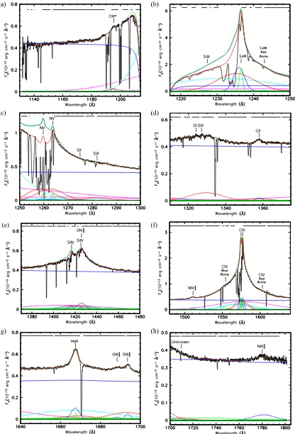
Figure1gives a detailed view of the best-fit model overlaid on the data. We illustrate all individual components of the model, the best-fit model overlaid on the data, and the absorption-corrected model(which is the ultimate goal of our
efforts). Note that the CIV absorption is not as deep in the mean spectrum from the reverberation campaign as it was during the deepest phase of the obscuration as observed in the XMM-Newtoncampaign(see Figure S1 in Kaastra et al.2014, which shows the individual components of the region surrounding the CIV emission line). For further illustrations of our model of the mean spectrum, see Figures1 and 2 of De Rosa et al.(2015), which compare the model to the full G130M and G160M spectra.
All of the model parameters are listed in Table1. The model consists of a total of 97 individual components, each with two to four parameters. Although the total number of parameters is 383, many of these are fixed or linked to other parameters. Free parameters in thefit total 143. Although this is a large number, the fit is tightly constrained. Thefitted regions in the mean spectrum comprise∼12,598 points, each approximately half of a resolution element. Thus, each spectrum has ∼6000 spectral elements included in thefit, and that is described by only 143 parameters. To optimize the parameters of the model and obtain the best fit, we use a combination of minimization algorithms. After determining initial guesses by visual inspection, we start the optimization process using a simplex algorithm (Murty
1983). This works well for problems with many parameters that are not initially well tuned. Once thefit is nearly optimized, this algorithm generally loses efficiency in approaching full convergence. At that point (usually after several tens of iterations), we switch to a Levenberg–Marquardt algorithm(as originally coded by Bevington 1969). When close to an optimum fit, this algorithm converges rapidly, but with the large number of parameters in ourfit, it can get stuck in false minima. To escape these pitfalls, we then alternate sets of 5–10 iterations using the simplex algorithm and the Levenberg– Marquardt algorithm until the fit has fully converged. We define full convergence as Δχ2<0.01 and a change in each parameter value of<1% after a set of iterations.
3.2. Modeling the Whole Time Series
Figure 1.(a)NGC 5548 mean COS spectrum, 1130–1214Å. The best-fit model for the COS UV spectrum of NGC 5548 is overlaid on the data(black). The total
Table 1
Model Parameters for the Mean Spectrum of NGC5548
Feature Componenta λvac λobs Fluxb FWHM Asymmetryc Freedomd
Number (Å) (Å) (km s−1) Flags
Power lawFλ(1000) 1 5.978e 0
Power lawα 1 0.840 0
E(B−V) 2 0.017 −1
RV 2 3.1 −1
Galactic Lyα 66 1215.67 1215.55 1.45f −1
CIII* 3 1175.78 1195.01 1.06 861 1.00 0, 0, 0,−1
CIII*B 95 1175.78 1195.01 3.13 3000 1.00 0, 0, 0,−1
SiIII 4 1206.50 1226.39 1.44 861 1.00 0, 0, 3,−1
Lyαnarrow 5 1215.67 1236.55 19.3 255 1.00 0, 0, 0,−1
Lyαintermediate 6 1215.67 1236.00 67.3 861 1.00 0, 0, 0,−1
LyαB 7 1215.67 1235.14 176.0 3047 1.00 0, 0, 0,−1
LyαMB 8 1215.67 1231.59 340.0 8074 1.00 0, 0, 0,−1
LyαVB 9 1215.67 1237.64 154.0 18347 1.00 0, 0, 0,−1
Lyαred bump 21 1215.67 1243.04 1.73 713 1.00 0, 0, 0,−1
NVnarrow 10 1238.82 1259.75 1.22 255 1.00 0, 0, 5,−1
NVnarrow 11 1242.80 1263.80 1.22 255 1.00 10, 10, 10,−1
NVintermediate 12 1238.82 1259.53 0.62 861 1.00 6, 0, 6,−1
NVintermediate 13 1242.80 1263.58 0.62 861 1.00 12, 12, 12,−1
NVB 14 1238.82 1258.66 23.3 3047 1.00 7, 0, 7,−1
NVB 15 1242.80 1262.70 23.3 3047 1.00 14, 14, 14,−1
NVMB 16 1238.82 1255.04 6.85 8074 1.00 8, 0, 8,−1
NVMB 17 1242.80 1259.08 6.85 8074 1.00 16, 16, 16,−1
NVVB 18 1240.01 1263.24 40.8 18347 1.00 9, 0, 9,−1
SII 19 1253.81 1273.00 0.09 841 1.00 0, 0, 0,−1
SiII 20 1260.42 1281.00 5.39 3500 1.00 0, 0, 0,−1
OInarrow 48 1302.17 1323.52 0.10 359 1.00 0, 0, 0,−1
SiIInarrow 49 1304.37 1327.01 0.20 359 1.00 0, 0, 48,−1
SiII+OIB 50 1303.27 1329.35 13.1 4659 1.00 0, 0, 0,−1
Unknown 47 K 1317.76 1.24 1687 1.00 0, 0, 0,−1
CIIintermediate 94 1334.53 1358.00 0.83 861 1.00 0, 0, 34,−1
CIIB 51 1334.53 1357.36 2.28 3000 1.00 0, 0,−1,−1
SiIVnarrow 96 1393.76 1416.74 0.41 303 1.00 0, 0, 0,−1
SiIVnarrow 97 1402.77 1425.90 0.20 303 1.00 96, 96, 96,−1
SiIVintermediate 23 1393.76 1415.97 1.67 842 1.00 0, 0, 0,−1
SiIVintermediate 24 1402.77 1425.13 0.84 842 1.00 23, 23, 23,−1
SiIVB 25 1393.76 1416.74 9.29 4889 1.00 0, 0, 0,−1
SiIVB 26 1402.77 1425.90 9.29 4889 1.00 25, 25, 25,−1
SiIVMB 27 1393.76 1415.28 12.5 8704 1.00 0, 0, 0,−1
SiIVMB 28 1402.77 1424.43 12.5 8704 1.00 27, 27, 27,−1
SiIVVB 29 1398.26 1409.20 37.1 18148 0.92 0, 0, 0,−1
OIV] 52 1400.00 1425.92 6.00 1858 1.00 0, 0, 0,−1
NIV]intermediate 39 1486.00 1510.54 3.30 1050 1.00 0, 0, 0,−1
NIV]B 22 1486.00 1512.13 1.83 3800 1.00 0, 0,−1,−1
CIVnarrow 30 1548.20 1574.34 7.86 303 1.00 0, 0, 0,−1
CIVnarrow 31 1550.77 1576.96 7.86 303 1.00 32, 32, 32,−1
CIVintermediate 32 1548.20 1574.32 21.4 861 1.00 0, 0, 0,−1
CIVintermediate 33 1550.77 1576.93 21.4 861 1.00 34, 34, 34,−1
CIVB 34 1548.20 1574.28 62.3 3366 1.00 0, 0, 0,−1
CIVB 35 1550.77 1576.90 62.3 3366 1.00 36, 36, 36,−1
CIVMB 36 1548.20 1569.00 98.5 8345 1.00 0, 0, 0,−1
CIVMB 37 1550.77 1571.61 98.5 8345 1.00 0, 0, 0,−1
CIVVB 38 1550.48 1577.99 286.0 16367 1.00 0, 0, 0,−1
CIVblue bump 93 1550.48 1553.79 7.53 1900 1.00 0, 0, 0,−1
CIVred bump 74 1550.48 1603.34 3.95 1708 1.00 0, 0, 0,−1
HeIInarrow 40 1640.45 1667.66 1.01 303 1.00 0, 0, 30,−1
HeIIintermediate 41 1640.45 1667.40 5.22 861 1.00 0, 0, 32,−1
HeIIB 42 1640.45 1669.07 6.18 3366 1.00 0, 0, 34,−1
HeIIMB 43 1640.45 1667.10 41.5 8345 1.00 0, 0, 36,−1
HeIIVB 67 1640.45 1667.14 4.93 16367 1.00 0, 0, 38,−1
OIII]narrow 92 1660.00 1686.82 0.87 771 1.00 0, 47, 0,−1
OIII]narrow 44 1666.00 1693.74 1.64 555 1.00 0, 0, 0,−1
OIII]B 45 1663.00 1693.23 13.5 3639 1.00 0, 0, 0,−1
PV region at the short-wavelength end. In the fits to the time series we discuss below, we use the values for the weak features determined from these grouped spectra as our initial guess for starting parameters whenfitting the individual spectra in a group. Another outcome of our trials, perhaps an obvious one, is that good initial choices for parameters led to quicker convergence and less chance of solutions where parameters strayed into unphysical regions of parameter space. Thus, given our exquisite fit to the mean spectrum, its parameters provide the best guess for spectra that are similar. To strengthen this similarity from fit to fit, we tried two different methods. First, we ordered the spectra by the flux level in the 1367Åcontinuum window. We then chose the spectrum near the middle of this distribution with theflux most
comparable to theflux in the mean spectrum as thefirst one tofit. The bestfit from this spectrum was then used as the initial guesses for parameters infitting the next spectra in the series. The series of fits followed two parallel paths moving both higher and lower in flux from this initial middle spectrum. Our second method was to keep the spectra ordered by time and then pick a spectrum close to the midpoint of the campaign with a mean continuum close to that of the mean spectrum. Fits then progressed both forward and backward in time from this middle point.
These experiments validated our intentions to develop an objective process for determining the bestfit to each spectrum. Both methods achieved good fits for all spectra, and the parameters from each method were close in value to each other Table 1
(Continued)
Feature Componenta λvac λobs Fluxb FWHM Asymmetryc Freedomd
Number (Å) (Å) (km s−1) Flags
NIII]B 46 1750.00 1781.33 7.56 3801 1.00 0, 0, 0,−1
FeII 53 K K 13.91g 1861.0 K −1, 0, 0,−1
CIII*broad absorption 54 1175.78 1194.00 −0.01 3796 0.13 0, 0, 55, 55
Lyαbroad absorption 55 1215.67 1235.00 −71.62 3796 0.13 0, 0, 0, 0
NVbroad absorption 56 1238.82 1258.00 −9.19 3796 0.13 0, 0, 55, 55
NVbroad absorption 57 1242.80 1262.04 −9.19 3796 0.13 56, 56, 55, 55
SIIbroad absorption 58 1253.81 1266.63 −0.94 3796 0.13 0, 0, 55, 55
SiIIbroad absorption 59 1260.42 1284.47 −0.93 3796 0.13 0, 0, 55, 55
SiIIbroad absorption 60 1304.37 1322.46 −0.18 3796 0.13 0, 0, 55, 55
CIIbroad absorption 61 1334.53 1355.00 −0.18 1761 0.26 0, 0, 0,−1
SiIVbroad absorption 62 1393.76 1415.20 −1.91 3796 0.13 0, 0, 55, 55
SiIVbroad absorption 63 1402.77 1424.36 −1.91 3796 0.13 62, 62, 55, 55
CIVbroad absorption 64 1548.20 1572.02 −5.18 2963 0.13 0, 0, 55, 55
CIVbroad absorption 65 1550.77 1574.63 −5.18 2963 0.13 64, 64, 55, 55
PVbroad absorption 69 1117.98 1136.00 −0.23 3796 0.65 0, 0, 55, 0
PVbroad absorption 70 1128.01 1146.19 −1.06 3796 0.65 0, 69, 69, 69
SiIIbroad absorption 71 1190.20 1212.26 −3.25 3796 0.13 0, 55, 55, 55
SiIIIbroad absorption 72 1206.50 1225.63 −0.94 3796 0.13 0, 55, 55, 55
SiIIbroad absorption 73 1526.71 1557.83 −1.92 3796 0.13 0, 55, 55, 55
CIIIbroad absorption 75 1175.78 1182.00 −0.31 1000 1.00 0,−1,−1,−1
Lyαbroad absorption 76 1215.67 1221.87 −1.80 1000 1.00 −1, 0,−1,−1
NVbroad absorption 77 1238.82 1245.14 −1.11 1000 1.00 −1, 0,−1,−1
NVbroad absorption 78 1242.80 1249.14 −1.11 1000 1.00 77,−1,−1,−1
SIIbroad absorption 79 1253.81 1260.20 −7.13 1000 1.00 76, 0,−1,−1
SiIIbroad absorption 80 1260.42 1266.93 −1.21 1000 1.00 76, 0,−1,−1
SiIIbroad absorption 81 1304.37 1310.65 0.00 1000 1.00 76, 0,−1,−1
CIIbroad absorption 82 1334.53 1341.81 −0.02 1000 1.00 76, 0,−1,−1
SiIVbroad absorption 83 1393.76 1405.00 −0.41 1000 1.00 76, 0,−1,−1
SiIVbroad absorption 84 1402.77 1414.09 −0.41 1000 1.00 83, 83,−1,−1
CIVbroad absorption 85 1548.20 1556.09 −0.74 1000 1.00 76, 0,−1,−1
CIVbroad absorption 86 1550.77 1558.68 −0.74 1000 1.00 85, 85,−1,−1
PVbroad absorption 87 1117.98 1136.00 −0.09 1000 1.00 76, 0,−1,−1
PVbroad absorption 88 1128.01 1146.19 −0.01 1000 1.00 76, 87,−1,−1
SiIIbroad absorption 89 1190.42 1199.38 0.00 1000 1.00 76, 0,−1,−1
SiIIIbroad absorption 90 1206.50 1212.61 0.00 1000 1.00 76, 0,−1,−1
SiIIbroad absorption 91 1526.71 1541.27 −0.19 1000 1.00 76, 0,−1,−1
Notes.
a
Component number in thespecfitmodel. Each component has multiple parameters as given in the table.
b
Flux is in 10−14ergcm−2s−1.
c
Asymmetry is defined as the ratio of the half-width at half-maximum of the red side of an asymmetric Gaussian to the half-width at half-maximum of the blue side.
d
Key for freedomflags: For each component,flags are given for each parameter—λobs,flux, FWHM, and asymmetry. Values correspond to the following:−1(fixed), 0(free),N>0(linked to corresponding parameter of componentN).
e
Flux is in 10−14ergcm−2s−1Å−1.
f
Column density is in 1020cm−2.
g
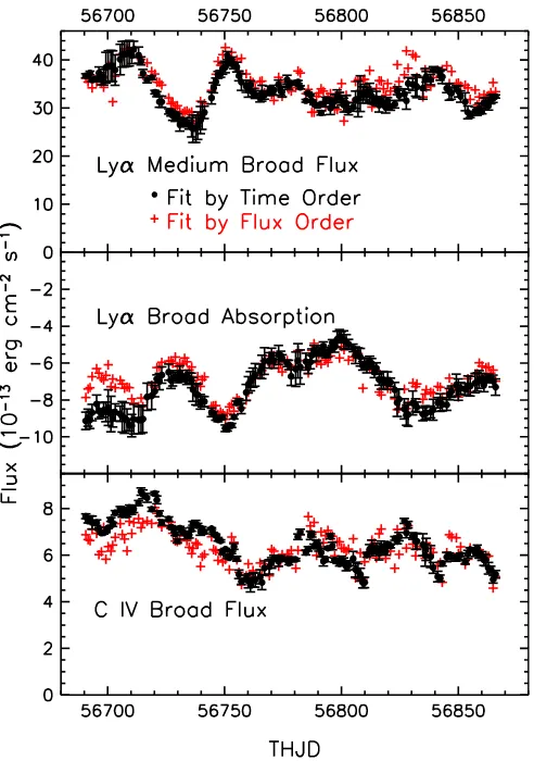
(typically within the 1σ uncertainties). Figure 2 compares the values obtained as a function of time for the two different methods for three selected parameters from the model. In Figure2and the remainder of the paper, we define times by the Truncated Heliocentric Julian Date(THJD), THJD=HJD−2,400,000.
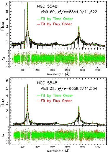
Despite the good agreement in the quality of thefits for the two different methods, our experiments also showed that the second method,“ordered by time,”produced better results than “ordered by flux,” in the sense that variations in parameter values were smoother, and, as shown in Figure3, the best-fitχ2 was typically slightly less. Despite the significant reduction in χ2we achieved for thefits ordered by time, the differences in thefits are not obvious. We note that for each method,χ2varies systematically with time during the campaign. The variations loosely correspond to the overall variations in brightness of NGC 5548(as one can see in laterfigures showing light curves for the continuum and emission line). Our inference for these systematic variations is that the brighter spectra have higher S/N per pixel, and that subtle residual pattern noise in thefl at-field properties of the COS detectors degrades the quality of our fits. Figure4 compares the best-fit models to the data for two extreme cases, our overall lowest χ2solution for visit 38 and our overall highestχ2obtained for visit 60. One is hard-pressed to see the differences between the models fit using either
method, or even why χ2 is significantly higher for visit 60 compared to visit 38.
Our best inference for why the“ordered by time”sequence produces better results is that the spectrum evolves on timescales of a few days. This is measured in the lags of the emission lines, and, as we will show later in Section 5.2, it is also true for the absorption features. Therefore, although one spectrum might have the same continuumflux as another, if it is separated in time by more than several days, the parameters of major features may differ significantly, making it harder for the minimization algorithm to converge on the best solution.
Tofit an individual spectrum, wefirst determined the bestfirst approximation to the normalization and spectral index of the power-law continuum byfitting only those points identified by De Rosa et al.(2015)as continuum windows. To avoid“ contaminat-ing”these windows with broad-lineflux, we also set theflux of all of the VB components to zero. In our experiments, we found that if we did not do this, the VB components developed a tendency to grow in width until they formed their own pseudo-continuum across the whole spectrum. In thisfirst pass, only the power-law normalization and index were allowed to vary freely.
After this step, we optimized the strength of the brightest emission lines—Lyα, NV, SiIV, CIV, and HeII—and let the fluxes of their B and MB components and the power-law normalization vary freely, while keeping the power-law index fixed and the VB component turned off. Next, we restored the VBfluxes to their original values, and let thefluxes of all broad components of the above lines vary freely, as well as the power-law normalization.
At this point, thefit formed a remarkably good representa-tion of an individual observarepresenta-tion, but it was still far from the bestfit. In the next steps, we turned our attention to optimizing the fits for each individual bright emission line. In these separate steps, we kept all parameters not related to the specific spectral regionfixed, including the continuum parameters, FeII
flux, narrow- and intermediate-line components for all lines, and any weak blended lines.
For the Lyαregion, we did separate optimization steps in the following order.
[image:10.612.47.293.49.399.2]Figure 2.Examples of the evolution of selected parameters comparing values obtained fromfits using time-ordered spectra(black points with error bars)to values from fits using flux-ordered spectra (red plus signs). The top panel shows the LyαMBflux, the middle panel shows the Lyαbroad absorption, and the bottom panel shows the CIVbroadflux.
Figure 3.Minimumχ2achieved in thefit to each spectrum in the campaign(upper curves and left axis). Black points show the results for our adopted method offitting the sequence of spectra in time order. Red points show the results forfitting the spectra when ordered byflux. The lower curves and right axis show the reducedχ2.
1. Fit Lyα only (B, MB, VB) using only wavelengths 1150–1245Å. As before, let the fluxes vary freelyfirst, then both the widths andfluxes. Keep all components of NVfixed throughout this.
2. Fit the red wing of NV using only wavelengths 1263–1300Å. Keep Lyαand all other componentsfixed. Let the two B components vary freelyfirst, thenfix them and let the MB components vary. Finally, fix those and let the VB component vary.
3. Fit the NV absorption on its blue wing, keeping the doublet’s fluxes tied at a 1:1 ratio, using only wavelengths 1245–1264Å.
4. Free the flux and width of the B, MB, and VB components of Lyα.
5. Free the flux and width of the B, MB, and VB components of NV.
6. Free theflux of the Lyα B absorber.
[image:11.612.124.490.50.566.2]We next did the SiIVregion. All parameters that we varied freely above for the optimization of the Lyαregion werefixed, and we then did the following.
1. Free theflux of the B, MB, and VB components of SiIV. 2. Free the flux and width of the B, MB, and VB
components of SiIV.
3. Free the flux of the SiIV B absorber. (Since the SiIV
absorption is so weak, we linked the width and asymmetry of the SiIVB absorber to that of CIV.) Wefit CIVand HeIItogether, since they are tightly blended. For optimizing this region, we fix all of the previous freely varying parameters, then do the following.
1. Free the flux and width of the B, MB, and VB components of CIV.
2. Free theflux(but not the width)of the B, MB, and VB components of HeII.
3. Free theflux of the CIVB absorber.
4. Free theflux, width, and asymmetry of the CIVB absorber. Once the major emission and absorption components are tuned up, we then allow the weaker emission-line features to adjust. We keep the continuum fixed, as well as all of the parameters associated with Lyα, NV, SiIV, CIV,and HeII. Thefluxes of all other weak emission features are then allowed to vary.
To complete the optimization, all parameters designated as free to vary in Table 1 are freed, and we iterate the χ2 minimization process until it converges. The best-fit parameters for this spectrum are then used as the initial guesses for doing thefit to the next spectrum in the series(with the exception that the initial guesses for the weak features are taken from the best fit to the grouped spectrum corresponding to that spectrum). Final values of all components as a function of wavelength for each spectrum are available as a high-level science product in the Mikulski Archive for Space Telescopes (MAST)114as the data set identified by10.17909/t9-ky1s-j932.
3.3. Propagating the Uncertainties
In principle, one can obtain 1σuncertainties on each of the parameters in our model from the best-fit covariance matrix. However, given the 383 parameters, 143 of which are freely varying, this is computationally impractical. An alternative is to assume that parameter space can be approximated by a parabola near the best-fit minimum in χ2. Using numerically calculatedfirst and second derivatives, one can then extrapolate from the minimum changes in each parameter to achieve
Δχ2=1, which corresponds to a 1σ uncertainty for a single interesting parameter (Bevington1969). Unfortunately, owing to the high dimensionality of our parameter space and its poor sampling in our calculations, this method proved inadequate.
All of the main quantities of interest to be extracted from our models are thefluxes of individual features, either in emission or in absorption. We therefore calculate uncertainties for these quantities using the data and associated uncertainties in each original spectrum and scaling them in proportion to the quantities that we integrate from our models. To explain this quantitatively,first we define these quantities:
fdata,i=flux in pixeliof the original spectrum,
σdata,i=1σ uncertainty for pixeliin the original spectrum,
fmod,i=flux in pixeliof the model spectrum,
σmod,i=1σuncertainty for pixel iin the model spectrum,
fc,j,i=flux in pixeliof the component j(of 97 total), and
σc,j=1σuncertainty for componentj.
Theflux of the model in pixelican be decomposed into the sum of the contributions of the individual components:
( )
å
=
f i f . 1
j c j i mod, , ,
The variance of the model in pixeliis then
( )
å
s i= s . 2
j c j mod, 2 , 2
In the limit of very good statistics, the variance predicted by the model should simply be the variance in the data themselves, i.e.,
( )
smod,i~s i, 3
2
data, 2
so the variance in the totalflux of any individual component is then ( ) ⎛ ⎝ ⎜⎜ ⎞ ⎠ ⎟⎟
å
å
s = s ´
¹
f f . 4
c j i
i i
k j c k i , 2 data, 2 mod, 2 , , 2
If the quantity of interest is the sum of multiple components
(i.e., the several components of an emission line contributing to the flux in a given velocity bin), then the 1σ uncertainty we derive for that quantity is
( )
å
s = s . 5
j c j
tot 2,
Figure 5 shows the consequences of this method for calculating the 1σuncertainties. When calculated directly from the data, as described above, the uncertainties are more uniform. The numerical instabilities in our method of interpolating in the error matrix of the fit give uncertainties that largely cluster around the calculation based on the data but show large excursions, both higher and lower.
Figure 5.Comparison of uncertainties for the broad Lyαabsorption feature in our model. Black points show the ratio of the uncertainty derived from the error matrix of the fit for Δχ2=1 divided by the 1σ uncertainty derived as described in Section3.3. The ratio scatters about unity(red line), with large excursions.
114
3.4. Quality Checking the Fits
The resulting best-fitχ2for each spectrum is shown as a time series in Figure3. The number of points in each spectrum varies slightly, since the spectrum is moved to multiple positions on the detector using different central wavelength settings. Because of the differing central wavelength settings, not all spectra cover the same range in wavelength as the mean spectrum; the settings tend to lose several hundred points on the blue and red ends of each spectrum. On average, individual spectra have∼11,600 points in eachfit. With 143 freely varying parameters, given theχ2values ranging from∼6800 to∼9000 in Figure3, one can see that our uncertainties are too large. This is most likely because in aligning and merging each spectrum, we have resampled the original pixels, introducing correlated errors in adjacent bins after rebinning. Note also that χ2 varies systematically with time in the campaign, largely following the light curve of total brightness. A likely explanation for this trend is that it is easier to get a good fit to our complex model when the fluxes are lower and uncertainties are larger.
While theχ2shows that we have goodfits overall, we visually examined each individual fit to see if there were any points or regions where there were systematic deviations of the model from the data. It was these inspections in our early experiments that led us to develop the fitting strategies we documented above. The finalfits show no gross or systematic residuals. This is illustrated visually by the image in Figure6that shows the residuals of Data
−Model for eachfit stacked into a two-dimensional spectrogram. The only significant features visible are the vertical lines at the positions of interstellar and intrinsic narrow absorption lines, which are not part of our model.
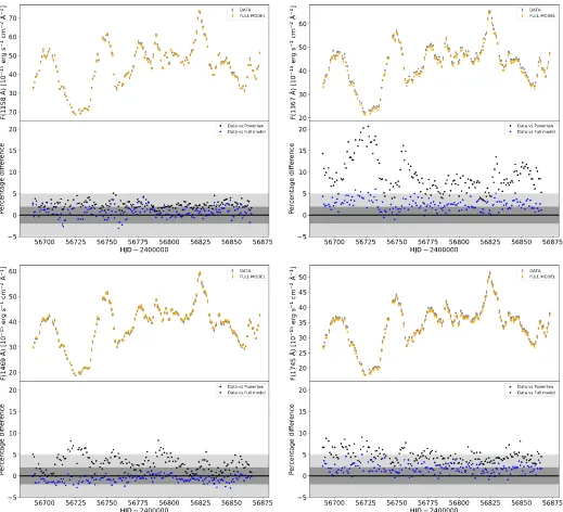
Ourfinal set of tests compared light curves offluxes extracted from our model fits to integrations of the same regions of data used in De Rosa et al.(2015). Again, here we see no systematic deviations, but these figures do illustrate how the continuum regions are slightly contaminated by wings of the broad emission lines. Figure 7 compares light curves for continuum windows integrated from the raw data, as described by De Rosa et al.
(2015), to integrations of the same wavelength regions in our models, both for the full model and for just the power-law continuum. The lower half of each panel in thefigure shows the differences between the two curves along with uncertainties from the raw data. These uncertainties include the systematic repeatability errors described by De Rosa et al.(2015)that apply to the time-series analysis offluxes from the campaign. These are
δP=1.1% for data with λ<1425Å and δP=1.4% for
λ>1425Å. One can see here that the cleanest continuum window, i.e., the one with the least contamination by surrounding emission lines, is the shortest-wavelength window surrounding 1158Å. Although this is the cleanest window in terms of total flux, we use the modeled continuum flux at 1367Å in our subsequent analysis. Since this is deterministically connected to the modeledflux at 1158Åthrough the continuum model, there is no difference between using one or the other.
3.5. The Absorption-corrected Spectra
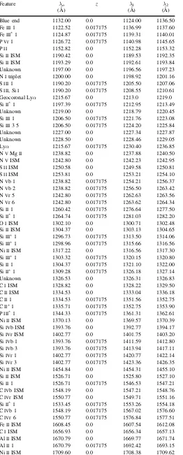
One of our main goals for thesefits to the emission model of each spectrum is to correct for the effects of intrinsic broad absorption and also to bridge the regions affected by foreground interstellar absorption lines and the narrow intrinsic absorption features in NGC 5548 itself. To correct for the broad absorption, we simply apply the inverse of these model elements to the data. For each pixel corrected in this way, we apply the same scaling to the associated uncertainty, as well as the data themselves. To correct for the narrow absorption features (both foreground and intrinsic), since these are not modeled, we replace the data in the wavelength regions affected by the absorption with the emission model.
More specifically, we first visually examine the fit to the mean spectrum to identify points that were significantly affected by narrow absorption lines. These intervals and their identifications are listed in Table 2. Next, we define the following quantities:
forig=flux in the original spectrum,
fmod=flux in the model spectrum (including broad absorption),
fabs=modelflux(negative)in the broad absorption lines, tG=transmission profile of Galactic damped Lyα, and fcor=flux in the corrected spectrum.
The corrected spectrum is then computed in two steps. First, we replace all pixels in the original spectrum withfcorif they fall within the wavelength intervals defined in Table 2. We then computefcor=(forig−fabs)/tG.
To calculate the 1σ uncertainties, we scale the original uncertainties in each pixel by the ratio of the correctedflux to the originalflux:
( ) ( )
3.6. Fluxes in Deblended Emission Lines
With our modelfits to the entire series of spectra from the STORM campaign, we can now extract absorption-corrected spectra for all emission lines across their full, deblended velocity profiles. Our models also allow us to separate the variable and nonvariable components of the strong emission lines, as well as deblend adjacent lines. For example, Crenshaw et al. (2009) were able to use the faint state of NGC 5548 in 2004 to separate and measure the narrow- and intermediate-line width components of the Lyα and CIV
emission lines. They demonstrated that these components vary only slightly over timescales of years. Using our model, we are able to exclude these nonvarying components of the emission lines from the overall broad-line profile. Likewise, we can separate the contributions of blended lines from the
wings of Lyα and CIV and measure lines such as NV as individual species.
For each individual broad emission line, we construct a model profile at each individual pixel ithat includes only the contributions of the relevant broad-line components from our model. As described in Section3.3, the netflux associated with a given emission feature is
( )
å
=
f i f , 7
j c j i totem, , ,
[image:14.612.48.567.49.521.2]the 1σ uncertainty on the data in that pixel,
( )
å
å
s =s f
f , 8
i i
j c j i
k c k i totem,
, , 2
, , 2
where the indexjruns over all components contributing to the desired emission feature, and the index k runs over all components of the model contributing to the flux in pixel i. As described in detail by De Rosa et al. (2015), systematic repeatability errors affect the data when considering a time-series analysis of these quantities. We therefore add in quadrature the same errors in precision, namely, δP=1.1%
for data from grating G130M(λ<1425Å)andδP=1.4% for
data from grating G160M (λ>1425Å). These errors in reproducibility actually dominate the uncertainties for all quantities atλ<1180 andλ>1425Å.
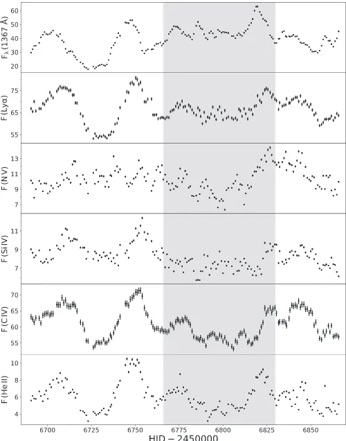
Figure8 compares light curves for the modeled continuum flux at 1367Åto the deblended broad emission lines of Lyα, NV, SiIV, CIV, and HeII. Portions of these light curves are tabulated in Table 3, with full tabulations of these quantities and the other continuum windows (1158, 1430, and 1740Å) available online. The light curves in Figure8closely resemble those derived from the original data shown in Figure3 of De Rosa et al.(2015). In general, Lyα, SiIV,and CIVare brighter due to the corrections for absorption, the additionalflux from the wings of the VB emission components, and the elimination of contaminating emission-line flux from the original con-tinuum windows. For HeII, the flux levels are roughly the same; additionalflux from the VB component of the emission line and a less contaminated continuum are offset by subtraction of blended emission from CIV. Overall, the error bars are smaller, since the modeled flux for any given component is determined by many more pixels than the limited wavelength range used in the original integrations. The light curve for NVis a new addition enabled by the deblending from Lyα in our model. In some respects, NVdiffers in character from the other emission lines, especially during the first 75 days of the campaign prior to the BLR holiday. However, starting with the BLR holiday, its behavior is very similar to that of CIVand HeII. We will quantify these similarities and differences in Section 4.1 when we discuss the emission-line lags.
3.7. Measuring the Absorption Lines
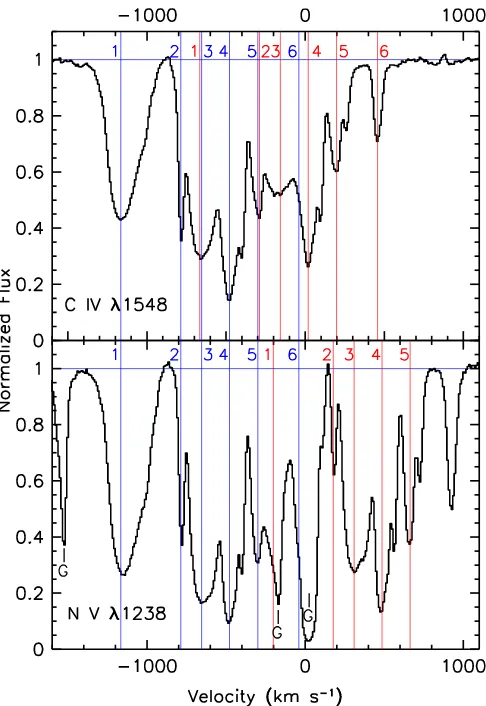
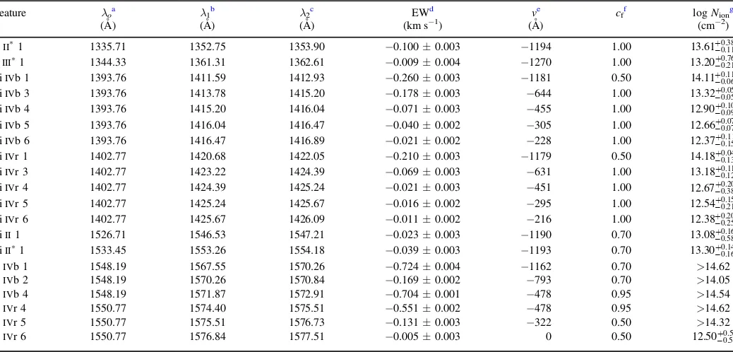
[image:15.612.44.306.89.740.2]The intrinsic narrow absorption lines comprise six discrete velocity components. We adopt the nomenclature of Mathur et al. (1999), numbering each component in order starting at the highest blueshifted velocity. To illustrate this kinematic structure, Figure9shows normalized absorption profiles for the most prominent intrinsic absorption lines as a function of velocity relative to the systemic velocity of the host galaxy Table 2
Wavelength Intervals for Correcting Narrow Absorption Features in the NGC 5548 Spectra
Feature λo z λ1 λ2
(Å) (Å) (Å)
Blue end 1132.00 0.0 1124.00 1136.50
FeIII1 1122.52 0.017175 1136.99 1137.60
FeIII*1 1124.87 0.017175 1139.31 1140.01
PVr 1 1126.72 0.017175 1140.98 1145.65
PII 1152.82 0.0 1152.28 1153.32
SiIIISM 1190.42 0.0 1189.53 1192.35
SiIIISM 1193.29 0.0 1192.61 1193.84
Unknown 1197.00 0.0 1196.56 1197.23
NItriplet 1200.00 0.0 1198.92 1201.16
SIII1 1190.20 0.017175 1205.50 1207.06
SIII, SiI 1190.20 0.017175 1208.55 1210.61
Geocoronal Lyα 1215.67 0.0 1213.0 1219.0
SiII*1 1197.39 0.017175 1212.95 1213.49
Unknown 1219.00 0.0 1218.79 1220.45
SiIII1 1206.50 0.017175 1221.76 1223.08
SiIII3 5 1206.50 0.017175 1224.20 1225.84
Unknown 1227.00 0.0 1227.34 1227.87
Unknown 1228.50 0.0 1228.46 1229.05
Lyα 1215.67 0.017175 1230.40 1236.85
NVMgII 1238.82 0.0 1237.88 1240.50
NVISM 1242.80 0.0 1242.23 1242.95
SIIISM 1250.58 0.0 1249.58 1250.81
SIIISM 1253.81 0.0 1253.21 1254.10
NVb 1 1238.82 0.017175 1254.21 1256.37
NVb 2 1238.82 0.017175 1256.50 1263.42
NVr 5 1242.80 0.017175 1262.63 1263.56
NVr 6 1242.80 0.017175 1263.62 1264.34
SiII1 1260.42 0.017175 1276.64 1277.50
SiII*1 1264.74 0.017175 1281.03 1282.20
OIISM 1302.10 0.0 1300.71 1302.48
SiIIISM 1304.37 0.0 1303.13 1304.65
SiIII*1 1296.73 0.017175 1313.50 1314.06
SiIII*1 1298.96 0.017175 1315.66 1316.56
NiIIISM 1317.22 0.0 1316.56 1317.30
SiIII*1 1303.32 0.017175 1320.15 1320.80
SiII1 1304.37 0.017175 1321.10 1322.00
SiII*1 1309.28 0.017175 1326.18 1327.14
Unknown 1326.53 0.0 1326.31 1326.83
CIISM 1328.82 0.0 1328.22 1329.50
CIIISM 1334.53 0.0 1333.04 1336.18
CII1 1334.53 0.017175 1351.56 1352.75
CII*1 1335.71 0.017175 1352.75 1353.90
PIII*1 1344.33 0.017175 1361.31 1362.61
NiIIISM 1370.13 0.0 1369.57 1370.39
SiIVb ISM 1393.76 0.0 1392.77 1394.17
SiIVr ISM 1402.77 0.0 1401.75 1403.20
SiIVb 1 1393.76 0.017175 1411.59 1412.80
SiIVb 3 1393.76 0.017175 1413.94 1417.11
SiIVr 1 1402.77 0.017175 1420.77 1422.14
SiIVr 3 1402.77 0.017175 1423.36 1426.35
NiIIISM 1454.84 0.0 1454.31 1455.10
SiIIISM 1526.71 0.0 1525.80 1527.10
SiII1 1526.71 0.017175 1546.53 1547.21
CIVb ISM 1548.19 0.0 1547.21 1548.76
CIVr ISM 1550.77 0.0 1549.71 1551.16
SiII*1 1533.45 0.017175 1553.26 1554.18
CIVb 1 1548.19 0.017175 1567.02 1576.60
CIVr 6 1550.77 0.017175 1576.84 1577.51
FeIIISM 1608.45 0.0 1607.54 1612.08
CIISM 1656.93 0.0 1656.34 1657.13
AlIIISM 1670.79 0.0 1669.77 1671.74
AlII1 1670.79 0.017175 1692.42 1693.15
NiIIISM 1709.60 0.0 1708.38 1709.62
Table 2 (Continued)
Feature λo z λ1 λ2
(Å) (Å) (Å)
NiIIISM 1741.55 0.0 1740.69 1741.72
NGC 5548. For this, we adopt the HI 21 cm redshift of z=0.017175(de Vaucouleurs et al.1991).
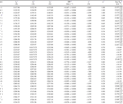
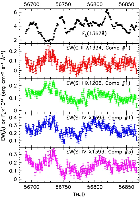
Measuring the strengths of the intrinsic narrow absorption lines is straightforward. Using the complete model of each spectrum (including the broad absorption components, since they help define the local continuum surrounding the narrow intrinsic absorption lines), we measure the equivalent widths
(EWs)by integrating across each absorption-line profile in the normalized spectrum. These integrations are performed as discrete sums over pixels lying within the wavelength regions defined for each feature in Table4:
( ) ( )
å
l= f -f f ´ D
EW . 9
i
i i i
orig, mod, mod,
The 1σuncertainty for EW is obtained by simply propagating the uncertainty associated with each data point in the original spectrum used in the sum:
( ) ( )
å
s = s f ´ Dl . 10
i
i i
EW orig,
2
orig,2 2
We use caution in performing these integrations to avoid features blended with Galactic absorption lines or other transitions. For example, the close velocity spacings of the CIV and NV doublets (498 and 964 km s−1, respectively) cause components 1, 2, 3, and 5 in CIV to overlap and components 1 and 5 in NVto overlap, as shown in Figure10. The red transition of component 1 in the NVdoublet is blended with Galactic SIIλ1259, and the blue transition of component 6 is blended with SiII λ1260. Therefore, Table 4 gives measurements only for clean, unblended features.
The EW of each broad absorption feature is calculated from the normalized modeled spectrum,
( ) ( )
=
-fnorm,i fmod,i fmod,i fabs,i , 11
as
( ) ( ) ( )
å
l l= -f ´ +
-EW 1 , 12
i
i i i
norm, 1
where λi is the wavelength of pixel i. Since our spectra are
[image:17.612.323.566.49.402.2]linearized, Δλ=λi+1−λi is actually a constant. The
Figure 9. Intrinsic narrow absorption features in NGC 5548. Normalized relative fluxes are plotted as a function of velocity relative to the systemic redshift ofz=0.017175. Thefirst panel shows Lyα, the second panel SiIII
[image:17.612.48.292.51.411.2]λ1206, the third panel SiIVλ1393(blue)and SiIVλ1402(red), the fourth panel CIVλ1548(blue)and CIVλ1550(red), and thefifth panel NVλ1238 (blue)and NVλ1242(red). Thin vertical lines indicate the velocities of the six intrinsic absorbers.