Multimodal Word Distributions

Proceedings of the 55th Annual Meeting of the Association for Computational Linguistics, pages 1645–1656

Proceedings of the 55th Annual Meeting of the Association for Computational Linguistics, pages 1645–1656

Multimodal Word Distributions

Ben Athiwaratkun Cornell University [email protected]

Andrew Gordon Wilson Cornell University [email protected]

Abstract

Word embeddings provide point represen-tations of words containing useful seman-tic information. We introduce multimodal word distributions formed from Gaussian mixtures, for multiple word meanings, en-tailment, and rich uncertainty informa-tion. To learn these distributions, we pro-pose an energy-based max-margin objec-tive. We show that the resulting approach captures uniquely expressive semantic in-formation, and outperforms alternatives, such as word2vec skip-grams, and Gaus-sian embeddings, on benchmark datasets such as word similarity and entailment.

1 Introduction

To model language, we must represent words. We can imagine representing every word with a binary one-hot vector corresponding to a dictio-nary position. But such a representation contains no valuable semantic information: distances be-tween word vectors represent only differences in alphabetic ordering. Modern approaches, by con-trast, learn to map words with similar meanings to nearby points in a vector space (Mikolov et al.,

2013a), from large datasets such as Wikipedia. These learned word embeddings have become ubiquitous in predictive tasks.

Vilnis and McCallum(2014) recently proposed an alternative view, where words are represented by a whole probability distribution instead of a de-terministic point vector. Specifically, they model each word by a Gaussian distribution, and learn its mean and covariance matrix from data. This approach generalizes any deterministic point em-bedding, which can be fully captured by the mean vector of the Gaussian distribution. Moreover, the full distribution provides much richer information

than point estimates for characterizing words, rep-resenting probability mass and uncertainty across a set of semantics.

However, since a Gaussian distribution can have only one mode, the learned uncertainty in this rep-resentation can be overly diffuse for words with multiple distinct meanings (polysemies), in or-der for the model to assign some density to any plausible semantics (Vilnis and McCallum,2014). Moreover, the mean of the Gaussian can be pulled in many opposing directions, leading to a biased distribution that centers its mass mostly around one meaning while leaving the others not well rep-resented.

In this paper, we propose to represent each word with an expressive multimodal distribution, for multiple distinct meanings, entailment, heavy tailed uncertainty, and enhanced interpretability. For example, one mode of the word ‘bank’ could overlap with distributions for words such as ‘fi-nance’ and ‘money’, and another mode could overlap with the distributions for ‘river’ and ‘creek’. It is our contention that such flexibility is critical for both qualitatively learning about the meanings of words, and for optimal performance on many predictive tasks.

In particular, we model each word with a mix-ture of Gaussians (Section 3.1). We learn all the parameters of this mixture model using a maximum margin energy-based ranking objective (Joachims, 2002; Vilnis and McCallum, 2014) (Section3.3), where the energy function describes the affinity between a pair of words. For analytic tractability with Gaussian mixtures, we use the in-ner product between probability distributions in a Hilbert space, known as the expected likelihood kernel (Jebara et al., 2004), as our energy func-tion (Secfunc-tion3.4). Additionally, we propose trans-formations for numerical stability and initializa-tionA.2, resulting in a robust, straightforward, and

scalable learning procedure, capable of training on a corpus with billions of words in days. We show that the model is able to automatically discover multiple meanings for words (Section 4.3), and significantly outperform other alternative meth-ods across several tasks such as word similarity and entailment (Section 4.4, 4.5, 4.7). We have made code available athttp://github.com/ benathi/word2gm, where we implement our model in Tensorflow (Abadi et. al, 2015).

2 Related Work

In the past decade, there has been an explo-sion of interest in word vector representations. word2vec, arguably the most popular word em-bedding, uses continuous bag of words and skip-gram models, in conjunction with negative sam-pling for efficient conditional probability estima-tion (Mikolov et al.,2013a,b). Other popular ap-proaches use feedforward (Bengio et al., 2003) and recurrent neural network language models (Mikolov et al., 2010, 2011b;Collobert and We-ston,2008) to predict missing words in sentences, producing hidden layers that can act as word em-beddings that encode semantic information. They employ conditional probability estimation tech-niques, including hierarchical softmax (Mikolov et al.,2011a;Mnih and Hinton,2008;Morin and Bengio, 2005) and noise contrastive estimation (Gutmann and Hyv¨arinen,2012).

A different approach to learning word em-beddings is through factorization of word co-occurrence matrices such as GloVeembeddings (Pennington et al., 2014). The matrix factoriza-tion approach has been shown to have an implicit connection with skip-gram and negative sampling

Levy and Goldberg (2014). Bayesian matrix fac-torization where row and columns are modeled as Gaussians has been explored inSalakhutdinov and Mnih(2008) and provides a different probabilistic perspective of word embeddings.

In exciting recent work, Vilnis and McCallum

(2014) propose a Gaussian distribution to model each word. Their approach is significantly more expressive than typical point embeddings, with the ability to represent concepts such as entailment, by having the distribution for one word (e.g. ‘mu-sic’) encompass the distributions for sets of related words (‘jazz’ and ‘pop’). However, with a uni-modal distribution, their approach cannot capture multiple distinct meanings, much like most

deter-ministic approaches.

Recent work has also proposed deterministic embeddings that can capture polysemies, for ex-ample through a cluster centroid of context vec-tors (Huang et al.,2012), or an adapted skip-gram model with an EM algorithm to learn multiple la-tent representations per word (Tian et al., 2014).

Neelakantan et al.(2014) also extends skip-gram with multiple prototype embeddings where the number of senses per word is determined by a non-parametric approach. Liu et al.(2015) learns topical embeddings based on latent topic models where each word is associated with multiple top-ics. Another related work byNalisnick and Ravi

(2015) models embeddings in infinite-dimensional space where each embedding can gradually repre-sent incremental word sense if complex meanings are observed.

Probabilistic word embeddings have only re-cently begun to be explored, and have so far shown great promise. In this paper, we propose, to the best of our knowledge, the first probabilistic word embedding that can capture multiple meanings. We use a Gaussian mixture model which allows for a highly expressive distributions over words. At the same time, we retain scalability and analytic tractability with an expected likelihood kernel en-ergy function for training. The model and train-ing procedure harmonize to learn descriptive rep-resentations of words, with superior performance on several benchmarks.

3 Methodology

In this section, we introduce our Gaussian mix-ture (GM) model for word representations, and present a training method to learn the parameters of the Gaussian mixture. This method uses an energy-based maximum margin objective, where we wish to maximize the similarity of distribu-tions of nearby words in sentences. We propose an energy function that compliments the GM model by retaining analytic tractability. We also pro-vide critical practical details for numerical stabil-ity and initialization. The code for model training and evaluation is available athttp://github. com/benathi/word2gm.

3.1 Word Representation

We represent each word w in a dictionary as a

Gaussian mixture with K components.

density

fw(~x) = K X

i=1

pw,iN[~x;~µw,i,Σw,i] (1)

=

K X

i=1

pw,i p

2π_|Σw,i|

e−12(~x−~µw,i)>Σ− 1

w,i(~x−~µw,i)_,

where PK_i=1pw,i = 1. The mean vectors ~µw,i represent the location of the ith component of

word w, and are akin to the point embeddings

provided by popular approaches likeword2vec.

pw,i represents the component probability (mix-ture weight), and Σw,i is the component covari-ance matrix, containing uncertainty information. Our goal is to learn all of the model parameters

~

µw,i, pw,i,Σw,ifrom a corpus of natural sentences to extract semantic information of words. Each Gaussian component’s mean vector of wordwcan

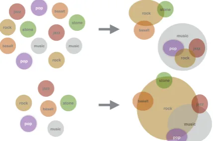
represent one of the word’s distinct meanings. For instance, one component of a polysemous word such as ‘rock’ should represent the meaning re-lated to ‘stone’ or ‘pebbles’, whereas another com-ponent should represent the meaning related to music such as ‘jazz’ or ‘pop’. Figure 1illustrates our word embedding model, and the difference be-tween multimodal and unimodal representations, for words with multiple meanings.

3.2 Skip-Gram

The training objective for learning θ = {~µw,i, pw,i,Σw,i} draws inspiration from the continuous skip-gram model (Mikolov et al.,

2013a), where word embeddings are trained to maximize the probability of observing a word given another nearby word. This procedure follows the distributional hypothesis that words occurring in natural contexts tend to be semanti-cally related. For instance, the words ‘jazz’ and ‘music’ tend to occur near one another more often than ‘jazz’ and ‘cat’; hence, ‘jazz’ and ‘music’ are more likely to be related. The learned word representation contains useful semantic informa-tion and can be used to perform a variety of NLP tasks such as word similarity analysis, sentiment classification, modelling word analogies, or as a preprocessed input for complex system such as statistical machine translation.

music

rock jazz

basalt

pop

stone

rock stone

jazz

pop

music basalt

music

jazz rock

basalt

pop

stone

rock

music

rock jazz

basalt

stone

pop

rock

basalt

stone

music jazz

pop

Figure 1: Top: A Gaussian Mixture embed-ding, where each component corresponds to a dis-tinct meaning. Each Gaussian component is rep-resented by an ellipsoid, whose center is specified by the mean vector and contour surface specified by the covariance matrix, reflecting subtleties in meaning and uncertainty. On the left, we show ex-amples of Gaussian mixture distributions of words where Gaussian components are randomly initial-ized. After training, we see on the right that one component of the word ‘rock’ is closer to ‘stone’ and ‘basalt’, whereas the other component is closer to ‘jazz’ and ‘pop’. We also demonstrate the entailment concept where the distribution of the more general word ‘music’ encapsulates words such as ‘jazz’, ‘rock’, ‘pop’.Bottom: A Gaussian embedding model (Vilnis and McCallum, 2014). For words with multiple meanings, such as ‘rock’, the variance of the learned representation becomes unnecessarily large in order to assign some proba-bility to both meanings. Moreover, the mean vec-tor for such words can be pulled between two clus-ters, centering the mass of the distribution on a re-gion which is far from certain meanings.

3.3 Energy-based Max-Margin Objective

Each sample in the objective consists of two pairs of words,(w, c)and(w, c0). wis sampled from a

sentence in a corpus andcis a nearby word within

a context window of length`. For instance, a word w =‘jazz’ which occurs in the sentence ‘I listen

to jazz music’ has context words (‘I’, ‘listen’, ‘to’ , ‘music’). c0is a negative context word (e.g.

‘air-plane’) obtained from random sampling.

The objective is to maximize the energy be-tween words that occur near each other,wandc,

and minimize the energy betweenwand its

neg-ative sampling (Mikolov et al., 2013a,b), which contrasts the dot product between positive context pairs with negative context pairs. The energy func-tion is a measure of similarity between distribu-tions and will be discussed in Section3.4.

We use a max-margin ranking objective (Joachims, 2002), used for Gaussian embeddings inVilnis and McCallum(2014), which pushes the similarity of a word and its positive context higher than that of its negative context by a marginm:

Lθ(w, c, c0) = max(0,

m₋logEθ(w, c) + logEθ(w, c0))

This objective can be minimized by mini-batch stochastic gradient descent with respect to the pa-rameters θ = {~µw,i, pw,i,Σw,i} – the mean vec-tors, covariance matrices, and mixture weights – of our multimodal embedding in Eq. (1).

Word Sampling We use a word sampling scheme similar to the implementation in word2vec (Mikolov et al., 2013a,b) to bal-ance the importbal-ance of frequent words and rare words. Frequent words such as ‘the’, ‘a’, ‘to’ are not as meaningful as relatively less frequent words such as ‘dog’, ‘love’, ‘rock’, and we are often more interested in learning the semantics of the less frequently observed words. We use subsampling to improve the performance of learning word vectors (Mikolov et al., 2013b). This technique discards wordwi with probability

P(wi) = 1 − p

t/f(wi), where f(wi) is the frequency of wordwi in the training corpus andt is a frequency threshold.

To generate negative context words, each word type wi is sampled according to a distribution

Pn(wi) ∝ U(wi)3/4 which is a distorted version of the unigram distributionU(wi)that also serves to diminish the relative importance of frequent words. Both subsampling and the negative distri-bution choice are proven effective inword2vec training (Mikolov et al.,2013b).

3.4 Energy Function

For vector representations of words, a usual choice for similarity measure (energy function) is a dot product between two vectors. Our word repre-sentations are distributions instead of point vec-tors and therefore need a measure that reflects not only the point similarity, but also the uncertainty. We propose to use theexpected likelihood kernel,

which is a generalization of an inner product be-tween vectors to an inner product bebe-tween distri-butions (Jebara et al.,2004). That is,

E(f, g) =

Z

f(x)g(x)dx=_hf, g_iL2

whereh·,_·iL2 denotes the inner product in Hilbert

spaceL2. We choose this form of energy since it can be evaluated in a closed form given our choice of probabilistic embedding in Eq. (1).

For Gaussian mixtures f, g representing the

words wf, wg, f(x) = PK_i=1piN(x;~µf,i,Σf,i) andg(x) = PK_i=1qiN(x;~µg,i,Σg,i),PK_i=1pi =

1, andPK_i=1qi = 1, we find (see SectionA.1) the log energy is

logEθ(f, g) = log K X

j=1 K X

i=1

piqjeξi,j (2)

where

ξi,j ≡logN(0;~µf,i−~µg,j,Σf,i+ Σg,j)

=₋1

2log det(Σf,i+ Σg,j)− D

2 log(2π)

−1₂(~µf,i−~µg,j)>(Σf,i+ Σg,j)−1(~µf,i−~µg,j) (3)

We call the termξi,j partial (log) energy. Observe that this term captures the similarity between the

ith _{meaning of word w}

f and the jth meaning of word wg. The total energy in Equation 2 is the sum of possible pairs of partial energies, weighted accordingly by the mixture probabilitiespiandqj. The term−(~µf,i−~µg,j)>(Σf,i+Σg,j)−1(~µf,i−

~

µg,j)inξi,jexplains the difference in mean vectors of semantic pair(wf, i)and(wg, j). If the seman-tic uncertainty (covariance) for both pairs are low, this term has more importance relative to other terms due to the inverse covariance scaling. We observe that the loss functionLθin Section3.3 at-tains a low value whenEθ(w, c)is relatively high. High values ofEθ(w, c)can be achieved when the component means across different words~µf,iand

~

At the beginning of training,ξi,jroughly are on the same scale among all pairs(i, j)’s. During this

time, all components learn the signals from the word occurrences equally. As training progresses and the semantic representation of each mixture becomes more clear, there can be one term ofξi,j’s that is predominantly higher than other terms, giv-ing rise to a semantic pair that is most related.

The negative KL divergence is another sensible choice of energy function, providing an asymmet-ric metasymmet-ric between word distributions. However, unlike the expected likelihood kernel, KL diver-gence does not have a closed form if the two dis-tributions are Gaussian mixtures.

4 Experiments

We have introduced a model for multi-prototype embeddings, which expressively captures word meanings with whole probability distributions. We show that our combination of energy and ob-jective functions, proposed in Section 3, enables one to learn interpretable multimodal distribu-tions through unsupervised training, for describing words with multiple distinct meanings. By rep-resenting multiple distinct meanings, our model also reduces the unnecessarily large variance of a Gaussian embedding model, and has improved re-sults on word entailment tasks.

To learn the parameters of the proposed mix-ture model, we train on a concatenation of two datasets: UKWAC (2.5 billion tokens) and Wackypedia (1 billion tokens) (Baroni et al.,

2009). We discard words that occur fewer than

100times in the corpus, which results in a

vocab-ulary size of314,129words. Our word sampling

scheme, described at the end of Section4.3, is sim-ilar to that ofword2vecwith one negative con-text word for each positive concon-text word.

After training, we obtain learned parameters

{~µw,i,Σw,i, pi}Ki=1 for each wordw. We treat the mean vector~µw,ias the embedding of theith mix-ture component with the covariance matrix Σw,i representing its subtlety and uncertainty. We per-form qualitative evaluation to show that our em-beddings learn meaningful multi-prototype repre-sentations and compare to existing models using a quantitative evaluation on word similarity datasets and word entailment.

We name our model as Word to Gaussian Mix-ture (w2gm) in constrast to Word to Gaussian (w2g) (Vilnis and McCallum, 2014). Unless

stated otherwise, w2g refers to our implementa-tion ofw2gmmodel with one mixture component.

4.1 Hyperparameters

Unless stated otherwise, we experiment withK = 2 components for thew2gm model, but we have results and discussion ofK = 3at the end of sec-tion 4.3. We primarily consider the spherical case for computational efficiency. We note that for di-agonal or spherical covariances, the energy can be computed very efficiently since the matrix inver-sion would simply requireO(d) computation

in-stead ofO(d3_{)for a full matrix. Empirically, we} have found diagonal covariance matrices become roughly spherical after training. Indeed, for these relatively high dimensional embeddings, there are sufficient degrees of freedom for the mean vec-tors to be learned such that the covariance matrices need not be asymmetric. Therefore, we perform all evaluations with spherical covariance models.

Models used for evaluation have dimension

D = 50 and use context window ` = 10unless

stated otherwise. We provide additional hyperpa-rameters and training details in the supplementary material (A.2).

4.2 Similarity Measures

Since our word embeddings contain multiple vec-tors and uncertainty parameters per word, we use the following measures that generalizes similarity scores. These measures pick out the component pair with maximum similarity and therefore deter-mine the meanings that are most relevant.

4.2.1 Expected Likelihood Kernel

A natural choice for a similarity score is the ex-pected likelihood kernel, an inner product between distributions, which we discussed in Section 3.4. This metric incorporates the uncertainty from the covariance matrices in addition to the similarity between the mean vectors.

4.2.2 Maximum Cosine Similarity

This metric measures the maximum similarity of mean vectors among all pairs of mixture com-ponents between distributions f and g. That is,

d(f, g) = max

i,j=1,...,K

hµf,i,µg,ji

||µf,i|| · ||µg,j||, which corre-sponds to matching the meanings off andg that

Word Co. Nearest Neighbors

rock 0 basalt:1, boulder:1, boulders:0, stalagmites:0, stalactites:0, rocks:1, sand:0, quartzite:1, bedrock:0 rock 1 rock/:1, ska:0, funk:1, pop-rock:1, punk:1, indie-rock:0, band:0, indie:0, pop:1

bank 0 banks:1, mouth:1, river:1, River:0, confluence:0, waterway:1, downstream:1, upstream:0, dammed:0 bank 1 banks:0, banking:1, banker:0, Banks:1, bankas:1, Citibank:1, Interbank:1, Bankers:0, transactions:1 Apple 0 Strawberry:0, Tomato:1, Raspberry:1, Blackberry:1, Apples:0, Pineapple:1, Grape:1, Lemon:0 Apple 1 Macintosh:1, Mac:1, OS:1, Amiga:0, Compaq:0, Atari:1, PC:1, Windows:0, iMac:0

star 0 stars:0, Quaid:0, starlet:0, Dafoe:0, Stallone:0, Geena:0, Niro:0, Zeta-Jones:1, superstar:0 star 1 stars:1, brightest:0, Milky:0, constellation:1, stellar:0, nebula:1, galactic:1, supernova:1, Ophiuchus:1 cell 0 cellular:0, Nextel:0, 2-line:0, Sprint:0, phones.:1, pda:1, handset:0, handsets:1, pushbuttons:0 cell 1 cytoplasm:0, vesicle:0, cytoplasmic:1, macrophages:0, secreted:1, membrane:0, mitotic:0, endocytosis:1 left 0 After:1, back:0, finally:1, eventually:0, broke:0, joined:1, returned:1, after:1, soon:0

left 1 right-hand:0, hand:0, right:0, left-hand:0, lefthand:0, arrow:0, turn:0, righthand:0, Left:0

Word Nearest Neighbors

rock band, bands, Rock, indie, Stones, breakbeat, punk, electronica, funk bank banks, banking, trader, trading, Bank, capital, Banco, bankers, cash Apple Macintosh, Microsoft, Windows, Macs, Lite, Intel, Desktop, WordPerfect, Mac

star stars, stellar, brightest, Stars, Galaxy, Stardust, eclipsing, stars., Star

cell cells, DNA, cellular, cytoplasm, membrane, peptide, macrophages, suppressor, vesicles left leaving, turned, back, then, After, after, immediately, broke, end

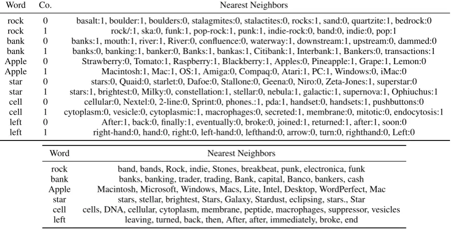
Table 1: Nearest neighbors based on cosine similarity between the mean vectors of Gaussian components for Gaussian mixture embedding (top) (forK = 2) and Gaussian embedding (bottom). The notationw:i denotes theithmixture component of the wordw.

4.2.3 Minimum Euclidean Distance

Cosine similarity is popular for evaluating em-beddings. However, our training objective di-rectly involves the Euclidean distance in Eq. (3), as opposed to dot product of vectors such as in word2vec. Therefore, we also consider the Eu-clidean metric:d(f, g) = min

i,j=1,...,K[||µf,i−µg,j||].

4.3 Qualitative Evaluation

In Table 1, we show examples of polysemous words and their nearest neighbors in the embed-ding space to demonstrate that our trained em-beddings capture multiple word senses. For in-stance, a word such as ‘rock’ that could mean ei-ther ‘stone’ or ‘rock music’ should have each of its meanings represented by a distinct Gaussian com-ponent. Our results for a mixture of two Gaussians model confirm this hypothesis, where we observe that the0th _{component of ‘rock’ being related to} (‘basalt’, ‘boulders’) and the1stcomponent being

related to (‘indie’, ‘funk’, ‘hip-hop’). Similarly, the wordbankhas its0th_{component representing} the river bank and the1st component representing

the financial bank.

By contrast, in Table 1 (bottom), see that for Gaussian embeddings with one mixture compo-nent, nearest neighbors of polysemous words are predominantly related to a single meaning. For in-stance, ‘rock’ mostly has neighbors related to rock

music and ‘bank’ mostly related to the financial bank. The alternative meanings of these polyse-mous words are not well represented in the embed-dings. As a numerical example, the cosine simi-larity between ‘rock’ and ‘stone’ for the Gaussian representation of Vilnis and McCallum(2014) is only0.029, much lower than the cosine similarity 0.586 between the 0th component of ‘rock’ and

‘stone’ in our multimodal representation.

In cases where a word only has a single popu-lar meaning, the mixture components can be fairly close; for instance, one component of ‘stone’ is close to (‘stones’, ‘stonework’, ‘slab’) and the other to (‘carving, ‘relic’, ‘excavated’), which re-flects subtle variations in meanings. In general, the mixture can give properties such as heavy tails and more interesting unimodal characterizations of un-certainty than could be described by a single Gaus-sian.

Embedding Visualization We provide an interactive visualization as part of our code

repos-itory: https://github.com/benathi/

word2gm#visualization that allows real-time queries of words’ nearest neighbors (in the embeddingstab) forK = 1,2,3components.

We use a notation similar to that of Table1, where a token w:i represents the component i of a word w. For instance, if in the K = 2 link we

neigh-bors such as river:1, confluence:0, waterway:1, which indicates that the 0th

component of ‘bank’ has the meaning ‘river bank’. On the other hand, searching forbank:1

yields nearby words such as banking:1,

banker:0, ATM:0, indicating that this com-ponent is close to the ‘financial bank’. We also have a visualization of a unimodal (w2g) for comparison in theK = 1link.

In addition, the embedding link for our Gaus-sian mixture model withK = 3mixture

compo-nents can learn three distinct meanings. For in-stance, each of the three components of ‘cell’ is close to (‘keypad’, ‘digits’), (‘incarcerated’, ‘in-mate’) or (‘tissue’, ‘antibody’), indicating that the distribution captures the concept of ‘cellphone’, ‘jail cell’, or ‘biological cell’, respectively. Due to the limited number of words with more than2

meanings, our model with K = 3does not

gen-erally offer substantial performance differences to our model withK = 2; hence, we do not further

displayK = 3results for compactness.

4.4 Word Similarity

We evaluate our embeddings on several standard word similarity datasets, namely, SimLex (Hill et al., 2014), WS or WordSim-353, WS-S (sim-ilarity), WS-R (relatedness) (Finkelstein et al.,

2002), MEN (Bruni et al.,2014), MC (Miller and Charles,1991), RG (Rubenstein and Goodenough,

1965), YP (Yang and Powers, 2006), MTurk(-287,-771) (Radinsky et al., 2011; Halawi et al.,

2012), and RW (Luong et al.,2013). Each dataset contains a list of word pairs with a human score of how related or similar the two words are.

We calculate the Spearman correlation ( Spear-man,1904) between the labels and our scores gen-erated by the embeddings. The Spearman corre-lation is a rank-based correcorre-lation measure that as-sesses how well the scores describe the true labels. The correlation results are shown in Table2 us-ing the scores generated from the expected like-lihood kernel, maximum cosine similarity, and maximum Euclidean distance.

We show the results of our Gaussian mixture model and compare the performance with that of word2vec and the original Gaussian em-bedding by Vilnis and McCallum (2014). We note that our model of a unimodal Gaussian embedding w2g also outperforms the original model, which differs in model

hyperparame-ters and initialization, for most datasets. Our multi-prototype modelw2gmalso performs better than skip-gram or Gaussian embedding methods on many datasets, namely, WS, WS-R, MEN, MC, RG, YP, MT-287, RW. The maximum cosine similarity yields the best performance on most datasets; however, the minimum Euclidean distance is a better metric for the datasets MC andRW. These results are consistent for both the single-prototype and the multi-prototype models.

We also compare out results on WordSim-353 with the multi-prototype embedding method by

Huang et al.(2012) andNeelakantan et al.(2014), shown in Table 3. We observe that our single-prototype modelw2g is competitive compared to models by Huang et al.(2012), even without us-ing a corpus with stop words removed. This could be due to the auto-calibration of importance via the covariance learning which decrease the impor-tance of very frequent words such as ‘the’, ‘to’, ‘a’, etc. Moreover, our multi-prototype model sub-stantially outperforms the model of Huang et al.

(2012) and the MSSG model ofNeelakantan et al.

(2014) on the WordSim-353 dataset.

4.5 Word Similarity for Polysemous Words

We use the dataset SCWS introduced by Huang et al. (2012), where word pairs are chosen to have variations in meanings of polysemous and homonymous words.

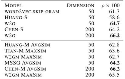
We compare our method with multiprototype models by Huang (Huang et al., 2012), Tian (Tian et al.,2014),Chen(Chen et al.,2014), and MSSG model by (Neelakantan et al., 2014). We note that Chen model uses an external lexical sourceWordNetthat gives it an extra advantage. We use many metrics to calculate the scores for the Spearman correlation. MaxSim refers to the maximum cosine similarity. AveSimis the aver-age of cosine similarities with respect to the com-ponent probabilities.

In Table 4, the model w2g performs the best among all single-prototype models for either 50

Dataset sg* w2g* w2g/mc w2g/el w2g/me w2gm/mc w2gm/el w2gm/me

SL 29.39 32.23 29.35 25.44 25.43 29.31 26.02 27.59

WS 59.89 65.49 71.53 61.51 64.04 73.47 62.85 66.39

WS-S 69.86 76.15 76.70 70.57 72.3 76.73 70.08 73.3

WS-R 53.03 58.96 68.34 54.4 55.43 71.75 57.98 60.13

MEN 70.27 71.31 72.58 67.81 65.53 73.55 68.5 67.7

MC 63.96 70.41 76.48 72.70 80.66 79.08 76.75 80.33

RG 70.01 71 73.30 72.29 72.12 74.51 71.55 73.52

YP 39.34 41.5 41.96 38.38 36.41 45.07 39.18 38.58

MT-287 - - 64.79 57.5 58.31 66.60 57.24 60.61

MT-771 - - 60.86 55.89 54.12 60.82 57.26 56.43

RW - - 28.78 32.34 33.16 28.62 31.64 35.27

Table 2: Spearman correlation for word similarity datasets. The models sg, w2g, w2gm denote word2vecskip-gram, Gaussian embedding, and Gaussian mixture embedding (K=2). The measures mc, el, medenote maximum cosine similarity, expected likelihood kernel, and minimum Euclidean distance. For each ofw2gandw2gm, we underline the similarity metric with the best score. For each dataset, we boldface the score with the best performance across all models. The correlation scores for sg*, w2g*are taken fromVilnis and McCallum(2014) and correspond to cosine distance.

MODEL ρ_×100

HUANG 64.2

HUANG* 71.3

MSSG 50D 63.2

MSSG 300D 71.2

W2G 70.9 W2GM 73.5

Table 3: Spearman’s correlation (ρ) on

WordSim-353 datasets for our Word to Gaussian Mixture embeddings, as well as the multi-prototype em-bedding by Huang et al. (2012) and the MSSG model byNeelakantan et al. (2014). Huang*is trained using data with all stop words removed. All models have dimension D = 50 except for

MSSG 300D withD = 300which is still

outper-formed by ourw2gmmodel.

probabilistic representation.

4.6 Reduction in Variance of Polysemous Words

One motivation for our Gaussian mixture embed-ding is to model word uncertainty more accurately than Gaussian embeddings, which can have overly large variances for polysemous words (in order to assign some mass to all of the distinct mean-ings). We see that our Gaussian mixture model does indeed reduce the variances of each compo-nent for such words. For instance, we observe that the wordrockinw2ghas much higher variance per dimension (e−1.8 ≈1.65) compared to that of

Gaussian components of rock in w2gm (which has variance of roughly e−2.5 _{≈ 0.82). We also}

MODEL DIMENSION ρ_×100

WORD2VEC SKIP-GRAM 50 61.7

HUANG-S 50 58.6

W2G 50 64.7

CHEN-S 200 64.2

W2G 200 66.2

HUANG-M AVGSIM 50 62.8

TIAN-M MAXSIM 50 63.6

W2GMMAXSIM 50 62.7

MSSG AVGSIM 50 64.2

CHEN-M AVGSIM 200 66.2

W2GMMAXSIM 200 65.5

Table 4: Spearman’s correlation ρ on dataset

SCWS. We show the results for single proto-type (top) and multi-protoproto-type (bottom) The suffix -(S,M) refers to single and multiple prototype models, respectively.

see, in the next section, that the Gaussian mixture model has desirable quantitative behavior for word entailment.

4.7 Word Entailment

We evaluate our embeddings on the word entail-ment dataset fromBaroni et al.(2012). The lexical entailment between words is denoted byw1|=w2 which means that all instances ofw1 arew2. The entailment dataset contains positive pairs such as

aircraft|=vehicleand negative pairs such as air-craft6|=insect.

max-MODEL SCORE BESTAP BESTF1 W2G(5) COS 73.1 76.4 W2G(5) KL 73.7 76.0 W2GM(5) COS 73.6 76.3

W2GM(5) KL 75.7 77.9

W2G(10) COS 73.0 76.1 W2G(10) KL 74.2 76.1

W2GM(10) COS 72.9 75.6

W2GM(10) KL 74.7 76.3

Table 5: Entailment results for models w2g and w2gm with window size 5 and10. The metrics

used are the maximum cosine similarity, or the maximum negative KL divergence. We calculate the best average precision as well as the best F1 score. In most cases,w2gmoutperformsw2gfor describing entailment.

imum cosine similarity and the minimum KL di-vergence, d(f, g) = min

i,j=1,...,KKL(f||g), for en-tailment scores. The minimum KL divergence is similar to the maximum cosine similarity, but also incorporates the embedding uncertainty. In addi-tion, KL divergence is an asymmetric measure, which is more suitable for certain tasks such as word entailment where a relationship is unidirec-tional. For instance, w1 |= w2 does not imply

w2|=w1. Indeed,aircraft|=vehicledoes not im-plyvehicle |=aircraft, since all aircraft are

vehi-cles but not all vehivehi-cles are aircraft. The difference betweenKL(w1||w2)versusKL(w2||w1) distin-guishes which word distribution encompasses an-other distribution, as demonstrated in Figure1.

Table 5 shows the results of ourw2gm model versus the Gaussian embedding model w2g. We observe a trend for both models with window size

5 and10 that the KL metric yields improvement

(both AP and F1) over cosine similarity. In ad-dition, w2gm has a better performance compared tow2g. The multi-prototype model estimates the meaning uncertainty better since it is no longer constrained to be unimodal, leading to better char-acterizations of entailment. On the other hand, the Gaussian embedding model suffers from large variance problem for polysemous words, which results in less informative word distribution and inferior entailment scores.

5 Discussion

We introduced a model that represents words with expressive multimodal distributions formed from Gaussian mixtures. To learn the properties of each

mixture, we proposed an analytic energy function for combination with a maximum margin objec-tive. The resulting embeddings capture different semantics of polysemous words, uncertainty, and entailment, and also perform favorably on word similarity benchmarks.

Elsewhere, latent probabilistic representations are proving to be exceptionally valuable, able to capture nuances such as face angles with varia-tional autoencoders (Kingma and Welling, 2013) or subtleties in painting strokes with the InfoGAN (Chen et al., 2016). Moreover, classically deter-ministic deep learning architectures are now being generalized to probabilistic deep models, for full predictive distributions instead of point estimates, and significantly more expressive representations (Wilson et al., 2016b,a;Al-Shedivat et al., 2016;

Gan et al.,2016;Fortunato et al.,2017).

Similarly, probabilistic word embeddings can capture a range of subtle meanings, and advance the state of the art in predictive tasks. Multimodal word distributions naturally represent our belief that words do not have single precise meanings: indeed, the shape of a word distribution can ex-press much more semantic information than any point representation.

In the future, multimodal word distributions could open the doors to a new suite of applica-tions in language modelling, where whole word distributions are used as inputs to new probabilis-tic LSTMs, or in decision functions where un-certainty matters. As part of this effort, we can explore different metrics between distributions, such as KL divergences, which would be a natu-ral choice for order embeddings that model entail-ment properties. It would also be informative to explore inference over the number of components in mixture models for word distributions. Such an approach could potentially discover an unbounded number of distinct meanings for words, but also distribute the support of each word distribution to express highly nuanced meanings. Alternatively, we could imagine a dependent mixture model where the distributions over words are evolving with time and other covariates. One could also build new types of supervised language models, constructed to more fully leverage the rich infor-mation provided by word distributions.

Acknowledgements

References

Maruan Al-Shedivat, Andrew Gordon Wilson, Yunus Saatchi, Zhiting Hu, and Eric P Xing. 2016. Learn-ing scalable deep kernels with recurrent structure. arXiv preprint arXiv:1610.08936.

Marco Baroni, Raffaella Bernardi, Ngoc-Quynh Do, and Chung-chieh Shan. 2012. Entailment above the word level in distributional semantics. InEACL 2012, 13th Conference of the European Chapter of the Association for Computational Linguistics, Avignon, France, April 23-27, 2012. pages 23–32. http://aclweb.org/anthology-new/E/E12/E12-1004.pdf.

Marco Baroni, Silvia Bernardini, Adriano Ferraresi, and Eros Zanchetta. 2009. The wacky wide web: a collection of very large linguistically processed web-crawled cor-pora. Language Resources and Evaluation 43(3):209– 226.https://doi.org/10.1007/s10579-009-9081-4. Yoshua Bengio, R´ejean Ducharme, Pascal Vincent, and

Christian Janvin. 2003. A neural probabilistic language model. Journal of Machine Learning Research3:1137– 1155.

Elia Bruni, Nam Khanh Tran, and Marco Baroni. 2014. Multimodal distributional semantics. J. Artif. Int. Res.

49(1):1–47.

Xi Chen, Xi Chen, Yan Duan, Rein Houthooft, John Schul-man, Ilya Sutskever, and Pieter Abbeel. 2016. Infogan: Interpretable representation learning by information maxi-mizing generative adversarial nets. InAdvances in Neural Information Processing Systems 29: Annual Conference on Neural Information Processing Systems 2016, Decem-ber 5-10, 2016, Barcelona, Spain. pages 2172–2180. Xinxiong Chen, Zhiyuan Liu, and Maosong Sun. 2014. A

unified model for word sense representation and disam-biguation. InProceedings of the 2014 Conference on Em-pirical Methods in Natural Language Processing, EMNLP 2014, October 25-29, 2014, Doha, Qatar, A meeting of SIGDAT, a Special Interest Group of the ACL. pages 1025– 1035.http://aclweb.org/anthology/D/D14/D14-1110.pdf. Ronan Collobert and Jason Weston. 2008. A unified

architec-ture for natural language processing: deep neural networks with multitask learning. InMachine Learning, Proceed-ings of the Twenty-Fifth International Conference (ICML 2008), Helsinki, Finland, June 5-9, 2008. pages 160–167. John C. Duchi, Elad Hazan, and Yoram Singer. 2011. Adap-tive subgradient methods for online learning and stochas-tic optimization. Journal of Machine Learning Research

12:2121–2159.

Mart´ın Abadi et al. 2015. TensorFlow: Large-scale machine learning on heterogeneous systems. Software available from tensorflow.org.

Lev Finkelstein, Evgeniy Gabrilovich, Yossi Matias, Ehud Rivlin, Zach Solan, Gadi Wolfman, and Eytan Ruppin. 2002. Placing search in context: the concept revisited.

ACM Trans. Inf. Syst.20(1):116–131.

Meire Fortunato, Charles Blundell, and Oriol Vinyals. 2017. Bayesian recurrent neural networks. arXiv preprint arXiv:1704.02798.

Zhe Gan, Chunyuan Li, Changyou Chen, Yunchen Pu, Qin-liang Su, and Lawrence Carin. 2016. Scalable bayesian learning of recurrent neural networks for language model-ing.arXiv preprint arXiv:1611.08034.

Michael Gutmann and Aapo Hyv¨arinen. 2012. Noise-contrastive estimation of unnormalized statistical models, with applications to natural image statistics. Journal of Machine Learning Research13:307–361.

Guy Halawi, Gideon Dror, Evgeniy Gabrilovich, and Yehuda Koren. 2012. Large-scale learning of word relatedness with constraints. InThe 18th ACM SIGKDD International Conference on Knowledge Discovery and Data Mining, KDD ’12, Beijing, China, August 12-16, 2012. pages 1406–1414.

Felix Hill, Roi Reichart, and Anna Korhonen. 2014. Simlex-999: Evaluating semantic models with (genuine) similar-ity estimation.CoRRabs/1408.3456.

Eric H. Huang, Richard Socher, Christopher D. Manning, and Andrew Y. Ng. 2012.Improving word representations via global context and multiple word prototypes. InThe 50th Annual Meeting of the Association for Computational Lin-guistics, Proceedings of the Conference, July 8-14, 2012, Jeju Island, Korea - Volume 1: Long Papers. pages 873– 882.http://www.aclweb.org/anthology/P12-1092. Tony Jebara, Risi Kondor, and Andrew Howard. 2004.

Prob-ability product kernels.Journal of Machine Learning Re-search5:819–844.

Thorsten Joachims. 2002. Optimizing search engines using clickthrough data. In Proceedings of the Eighth ACM SIGKDD International Conference on Knowledge Discov-ery and Data Mining, July 23-26, 2002, Edmonton, Al-berta, Canada. pages 133–142.

Diederik P. Kingma and Jimmy Ba. 2014. Adam: A method for stochastic optimization.CoRRabs/1412.6980. Diederik P. Kingma and Max Welling. 2013.

Auto-encoding variational bayes. CoRR abs/1312.6114.

http://arxiv.org/abs/1312.6114.

Y. LeCun, L. Bottou, G. Orr, and K. Muller. 1998. Efficient backprop. In G. Orr and Muller K., editors,Neural Net-works: Tricks of the trade. Springer.

Omer Levy and Yoav Goldberg. 2014. Neural word em-bedding as implicit matrix factorization. InAdvances in Neural Information Processing Systems 27: Annual Con-ference on Neural Information Processing Systems 2014, December 8-13 2014, Montreal, Quebec, Canada. pages 2177–2185.

Yang Liu, Zhiyuan Liu, Tat-Seng Chua, and Maosong Sun. 2015. Topical word embeddings. In

Proceedings of the Twenty-Ninth AAAI Confer-ence on Artificial IntelligConfer-ence, January 25-30, 2015, Austin, Texas, USA.. pages 2418–2424.

http://www.aaai.org/ocs/index.php/AAAI/AAAI15/paper/view/9314. Minh-Thang Luong, Richard Socher, and Christopher D.

Manning. 2013. Better word representations with recur-sive neural networks for morphology. In CoNLL. Sofia, Bulgaria.

Tomas Mikolov, Anoop Deoras, Daniel Povey, Luk´as Burget, and Jan Cernock´y. 2011a. Strategies for training large scale neural network language mod-els. In 2011 IEEE Workshop on Automatic Speech Recognition & Understanding, ASRU 2011, Waikoloa, HI, USA, December 11-15, 2011. pages 196–201.

https://doi.org/10.1109/ASRU.2011.6163930.

Tomas Mikolov, Martin Karafi´at, Luk´as Burget, Jan Cer-nock´y, and Sanjeev Khudanpur. 2010. Recurrent neu-ral network based language model. In INTERSPEECH 2010, 11th Annual Conference of the International Speech Communication Association, Makuhari, Chiba, Japan, September 26-30, 2010. pages 1045–1048.

Tomas Mikolov, Stefan Kombrink, Luk´as Burget, Jan Cernock´y, and Sanjeev Khudanpur. 2011b. Exten-sions of recurrent neural network language model. In Proceedings of the IEEE International Confer-ence on Acoustics, Speech, and Signal Processing, ICASSP 2011, May 22-27, 2011, Prague Congress Center, Prague, Czech Republic. pages 5528–5531.

https://doi.org/10.1109/ICASSP.2011.5947611.

Tomas Mikolov, Ilya Sutskever, Kai Chen, Gregory S. Cor-rado, and Jeffrey Dean. 2013b. Distributed representa-tions of words and phrases and their compositionality. In

Advances in Neural Information Processing Systems 26: 27th Annual Conference on Neural Information Process-ing Systems 2013. ProceedProcess-ings of a meetProcess-ing held Decem-ber 5-8, 2013, Lake Tahoe, Nevada, United States.. pages 3111–3119.

George A. Miller and Walter G. Charles. 1991.

Contextual Correlates of Semantic Similarity.

Language & Cognitive Processes 6(1):1–28.

https://doi.org/10.1080/01690969108406936.

Andriy Mnih and Geoffrey E. Hinton. 2008. A scalable hi-erarchical distributed language model. In Advances in Neural Information Processing Systems 21, Proceedings of the Twenty-Second Annual Conference on Neural Infor-mation Processing Systems, Vancouver, British Columbia, Canada, December 8-11, 2008. pages 1081–1088. Frederic Morin and Yoshua Bengio. 2005. Hierarchical

prob-abilistic neural network language model. InProceedings of the Tenth International Workshop on Artificial Intelli-gence and Statistics, AISTATS 2005, Bridgetown, Barba-dos, January 6-8, 2005.

Eric T. Nalisnick and Sachin Ravi. 2015. Infinite dimensional word embeddings.CoRRabs/1511.05392.

Arvind Neelakantan, Jeevan Shankar, Alexandre Passos, and Andrew McCallum. 2014. Efficient non-parametric esti-mation of multiple embeddings per word in vector space. In Proceedings of the 2014 Conference on Empirical Methods in Natural Language Processing, EMNLP 2014, October 25-29, 2014, Doha, Qatar, A meeting of SIGDAT, a Special Interest Group of the ACL. pages 1059–1069.

http://aclweb.org/anthology/D/D14/D14-1113.pdf. Jeffrey Pennington, Richard Socher, and Christopher D.

Manning. 2014. Glove: Global vectors for word repre-sentation. InProceedings of the 2014 Conference on Em-pirical Methods in Natural Language Processing, EMNLP 2014, October 25-29, 2014, Doha, Qatar, A meeting of SIGDAT, a Special Interest Group of the ACL. pages 1532– 1543.http://aclweb.org/anthology/D/D14/D14-1162.pdf.

Kira Radinsky, Eugene Agichtein, Evgeniy Gabrilovich, and Shaul Markovitch. 2011. A word at a time: Comput-ing word relatedness usComput-ing temporal semantic analysis. In Proceedings of the 20th International Conference on World Wide Web. WWW ’11, pages 337–346.

Herbert Rubenstein and John B. Goodenough. 1965. Contex-tual correlates of synonymy. Commun. ACM8(10):627– 633.

Ruslan Salakhutdinov and Andriy Mnih. 2008. Bayesian probabilistic matrix factorization using markov chain monte carlo. In Machine Learning, Proceedings of the Twenty-Fifth International Conference (ICML 2008), Helsinki, Finland, June 5-9, 2008. pages 880–887.

https://doi.org/10.1145/1390156.1390267.

C. Spearman. 1904. The proof and measurement of associa-tion between two things.American Journal of Psychology

15:88–103.

Fei Tian, Hanjun Dai, Jiang Bian, Bin Gao, Rui Zhang, Enhong Chen, and Tie-Yan Liu. 2014. A probabilistic model for learning multi-prototype word embeddings. In

COLING 2014, 25th International Conference on Com-putational Linguistics, Proceedings of the Conference: Technical Papers, August 23-29, 2014, Dublin, Ireland. pages 151–160. http://aclweb.org/anthology/C/C14/C14-1016.pdf.

Luke Vilnis and Andrew McCallum. 2014. Word representa-tions via gaussian embedding.CoRRabs/1412.6623.

Andrew G Wilson, Zhiting Hu, Ruslan R Salakhutdinov, and Eric P Xing. 2016a. Stochastic variational deep kernel learning. InAdvances in Neural Information Processing Systems. pages 2586–2594.

Andrew Gordon Wilson, Zhiting Hu, Ruslan Salakhutdinov, and Eric P Xing. 2016b. Deep kernel learning. In Pro-ceedings of the 19th International Conference on Artificial Intelligence and Statistics. pages 370–378.

Dongqiang Yang and David M. W. Powers. 2006. Verb sim-ilarity on the taxonomy of wordnet. InIn the 3rd Interna-tional WordNet Conference (GWC-06), Jeju Island, Korea.

A Supplementary Material

A.1 Derivation of Expected Likelihood Kernel

We derive the form of expected likelihood kernel for Gaussian mixtures. Let f, g be Gaussian mixture distributions representing the words wf, wg. That

is, f(x) = PK_i=1piN(x;µf,i,Σf,i) and g(x) =

PK

i=1qiN(x;µg,i,Σg,i),

PK

i=1pi= 1, and

PK

The expected likelihood kernel is given by

Eθ(f, g) =

Z _XK

i=1

piN(x;µf,i,Σf,i) !

·

K X

j=1

qjN(x;µg,j,Σg,j) !

dx

= K X

i=1 K X

j=1 piqj

Z

N(x;µf,i,Σf,i)· N(x;µg,j,Σg,j)dx

= K X

i=1 K X

j=1

piqjN(0;µf,i−µg,j,Σf,i+ Σg,j)

= K X

i=1 K X

j=1 piqjeξi,j

where we note that RN(x;µi,Σi)N(x;µj,Σj) dx =

N(0, µi−µj,Σi+ Σj)(Vilnis and McCallum,2014) and ξi,jis the log partial energy, given by equation 3.

A.2 Implementation

In this section we discuss practical details for training the pro-posed model.

Reduction to Diagonal Covariance

We use a diagonalΣ, in which case inverting the covariance matrix is trivial and computations are particularly efficient.

Letdf_,dg_{denote the diagonal vectors ofΣf,ΣgThe}

ex-pression forξi,jreduces to

ξi,j=−1 2

D X

r=1

log(dpr+dqr)

−1₂X (µp,i−µq,j)◦ 1

dp_+dq ◦(µp,i−µq,j)

where◦denotes element-wise multiplication. The spherical case which we use in all our experiments is similar since we simply replace a vectordwith a single value.

Optimization Constraint and Stability

We optimizelogdsince each component of diagonal vector

dis constrained to be positive. Similarly, we constrain the probabilitypito be in[0,1]and sum to1by optimizing over

unconstrained scoressi ∈ (−∞,∞)and using a softmax

function to convert the scores to probabilitypi= PKesi j=1esj.

The loss computation can be numerically unstable if ele-ments of the diagonal covariances are very small, due to the termlog(df

r +dgr)and dq₊1_dp. Therefore, we add a small

constant = 10−4 so thatdfr +dgr anddq+dpbecomes df

r+dgr+anddq+dp+.

In addition, we observe thatξi,jcan be very small which

would result ineξi,j ≈0up to machine precision. In order to

stabilize the computation in eq.2, we compute its equivalent form

logE(f, g) =ξi0,j0+ log K X

j=1 K X

i=1

piqjeξi,j−ξi0,j0

whereξi0,j0= maxi,jξi,j.

Model Hyperparameters and Training Details

In the loss functionLθ, we use a marginm= 1and a batch

size of128. We initialize the word embeddings with a uni-form distribution over[−q3

D, q

3

D]so that the expectation

of variance is1and the mean is zero (LeCun et al.,1998). We initialize each dimension of the diagonal matrix (or a sin-gle value for spherical case) with a constant valuev= 0.05. We also initialize the mixture scoressi to be0so that the

initial probabilities are equal among allKcomponents. We use the thresholdt= 10−5 _{for negative sampling, which is}

the recommended value forword2vecskip-gram on large datasets.

We also use a separate output embeddings in addition to input embeddings, similar toword2vecimplementation (Mikolov et al.,2013a,b). That is, each word has two sets of distributionsqIandqO, each of which is a Gaussian mixture.

For a given pair of word and context(w, c), we use the input

distributionqIforw(input word) and the output distribution qOfor contextc(output word). We optimize the parameters

of bothqIandqO and use the trained input distributionsqI

as our final word representations.

We use mini-batch asynchronous gradient descent with Adagrad (Duchi et al.,2011) which performs adaptive learn-ing rate for each parameter. We also experiment with Adam (Kingma and Ba,2014) which corrects the bias in adaptive gradient update of Adagrad and is proven very popular for most recent neural network models. However, we found that it is much slower than Adagrad (≈ 10times). This is because the gradient computation of the model is relatively fast, so a complex gradient update algorithm such as Adam becomes the bottleneck in the optimization. Therefore, we choose to use Adagrad which allows us to better scale to large datasets. We use a linearly decreasing learning rate from0.05