Open Journal of Statistics, 2011, 1, 161-171
doi:10.4236/ojs.2011.13020 Published Online October 2011 (http://www.SciRP.org/journal/ojs)
161
Estimation of the Unknown Parameters for the Compound
Rayleigh Distribution Based on Progressive
First-Failure-Censored Sampling
Tahani A. Abushal
Department of Mathematics, Umm Al-Qura University, Makkah Al-Mukarramah, KSA E-mail: [email protected]
Received August 2, 2011; revised September 5, 2011; accepted September 17,2011
Abstract
This article considers estimation of the unknown parameters for the compound Rayleigh distribution (CRD) based on a new life test plan called a progressive first failure-censored plan introduced by Wu and Kus (2009). We consider the maximum likelihood and Bayesian inference of the unknown parameters of the model, as well as the reliability and hazard rate functions. This was done using the conjugate prior for the shape parameter, and discrete prior for the scale parameter. The Bayes estimators have been obtained relative to both symmetric (squared error) and asymmetric (LINEX and general entropy (GE) loss functions. It has been seen that the symmetric and asymmetric Bayes estimators are obtained in closed forms. Also, based on this new censoring scheme, approximate confidence intervals for the parameters of CRD are developed. A practical example using real data set was used for illustration. Finally, to assess the performance of the pro-posed estimators, some numerical results using Monte Carlo simulation study were reported.
Keywords:Compound Rayleigh Distribution, Progressive First-Failure Censored Scheme, Bayesian and Non-Bayesian Estimations, Approximate Confidence Intervals
1. Introduction
There are many scenarios in life-testing and reliability experiments whose units are lost or removed from ex-perimentation before failure. The loss may occur unin-tentionally, or it may have been designed so in the study. However, in many situations, the removal of units prior to failure is preplanned in order to provide saving in terms of time and cost associated with testing. There are many types of censored test, the most common censoring schemes are type-I and type-II censoring, but using this types of censoring can not allow for units to be removed from the test at any other point than the final termination point. However, if an experimenter desires to remove surviving units at points other than the final termination point of the life test, these two traditional censoring schemes will not be of use to the experimenter. The al-lowance of removing surviving units from the test before the final termination point is desirable, as in the case of studies of wear, in which the study of the actual aging process requires units to be fully disassembled at differ-ent stages of the experimdiffer-ent. In addition, when a
com-promise between the reduced time of experimentation and the observation of at least some extreme lifetimes is sought, such an allowance is also desirable. These rea-sons lead us into the area of progressive censoring.
It is well known that one of the primary goals of pro-gressive censoring is to save some live units for other tests, which is particularly useful when the units being tested are very expensive. [1] mentioned that the infer-ence is feasible, and practical when the sample data are gathered according to a Type-II progressively censored study experimental scheme. Statistical inferences on the parameters of failure time distributions under progressive censoring have been studied by several authors such as [1-12]. A recent account on progressive censoring sche- mes can be found in the book by [13], or in the excellent review by [14].
bear-ing manufacturer. The bearbear-ing test engineer decided to save test time by testing 50 bearings in sets of 10 each, and the first-failure times from each group were ob-served. [17,18] discussed some inferences based on first- failure-censored sampling from both the Gompertz dis-tribution and Burr-XII disdis-tribution, respectively. Also see [19,20]. Note that a first-failure-censoring scheme is terminated when the first failure in each set is observed. If an experimenter desires to remove some sets of test units before observing the first failures in these sets this life test plan is called a progressive first-failure-censor- ing scheme which recently introduced by [21].
The two-parameter compound Rayleigh distribution (which is denoted by CRD ( , )
)
) provides a popula-tion model which is useful in several areas of statistics, including life testing and reliability. The probability den-sity function ( , and the cumulative distribution function of CRD ( ,
)
)
(cdf are given, respectively,
by
2 ( 1)
( ) = 2 ( ) ,
> 0, > 0, > 0,
f x x x
x
(1)
2
( ) = 1 ( )
F x x , (2)
and the reliability and failure rate functions, at some , are
t
2
( ) = ( )
S t t , t> 0, (3)
2
2 ( ) = t
H t
t
, t> 0, (4)
where and are the shape and the scale parameter respectively.
The compound Rayleigh distribution (CRD) is a spe-cial case of the 3- parameter Burr type XII distribution, which has a PDF of the form. The 2- parameter version of this distribution (with) was studied by several authors, such as [22-26], among others.
The main aim of this article is to focus on the design-ing problem of a progressive first-failure censordesign-ing life test with a compound Rayleigh failure time distribution. The rest of this article is organized as follows. In Section 2, the formulation of a progressive first-failure-censoring scheme is described. The ML estimations with the ap-proximate confidence intervals of the parameters are obtained in Section 3. Bayesian estimations of the pa-rameters, reliability and hazard rate functions of CRD based on progressive first-failure-censoring scheme are investigated in Section 4. In Section 5, for illustrative purposes, we performed a real data analysis. A simula-tion study in order to give an assessment of the perform-ance of the estimation methods are presented in Section 6. Finally we conclude the paper in Section 7.
2. A Progressive First-Failure-Censoring
Scheme
In this section, first-failure-censoring scheme is com-bined with the progressive censoring scheme as in [21]. Suppose that independent groups with items within each group are put in a life test, 1 groups and
the group in which the first failure is observed are ran-domly removed from the test as soon as the first failure (say 1: : :m n k) has occurred, 2 groups and the group in
which the second first failure is observed are randomly removed from the test when the second failure (say
2: : :m n k) has occurred, and finally m groups and the group in which the first failure is ob-served are randomly removed from the test as soon as the
n k
n R
(
R m
XR R
XR )
m th
m th failure (say : : : ) has occurred. The 1: : :m n k
2: : : m m n k: : : are called progressively first-
failure-censored order statistics with the progressive
cen-soring scheme . It is clear that
m m n k
XR XR
1 2
= R R, ,
XR < XR <<
R (
m
m n k
,Rm)
=1
= i
j
n m
R . If the failure times of the n k items originally in the test are from a continuous population with distribution function F x( ) and probability density function f x( )R R
, the joint probability density function for
1: : :m n k, 2: : :m n k, , m m n k: : :
X X XR is given by
1,2,..., 1: : : 2: : : : : :
( 1) 1 : : : : : :
=1
( , ,..., )
= ( ) 1 ( )
m m n k m n k m m n k
m k
j j m n k j m n k j
f x x x
Ck
f x F x ,R R R
R
R R (5)
1: : : 2: : : : : :
0 <xm n k <x m n k < ... <xm m n k <
R R R ,
where
1 1 2
1 2 1
= ( 1)( 1)
( m 1).
C n n R n R R
n R R R m
(6)
It should be noted that 1; , , 2; , , ; , ,
can be viewed as a progressive type II censored sample from a population with distribution function 1 (
, , ,
m n k m n k m m n k
XR XR XR
1
( ))k
F x . For this reason, results for progressive type II
censored order statistics can be extended to progressive first-failure censored order statistics easily. Also, the progressive first-failure censored plan has advantages in terms of reducing the test time, in which more items are used, but only m of n k items are failures.
3. Maximum Likelihood Estimation
Based on progressively first-failure-censored sample
: : :
i m n k, , with censoring scheme is
drawn from the CRD (1). For convenience, we will de-note the observed values of such sample by i
XR i= 1, 2, , m R
X ,
. From (5), the likelihood function is given by = 1
i ,
163 T. A. ABUSHAL
2
2
=1 =1
( , ) = (2 )
exp ( 1) log ,
m kn
m m
i
i i
i i i
L C k
x
k R x
x
(7)where is defined in (6) The log-likelihood function is given by
C
2 2
=1 =1
( , ) = log (2 ) log log
log ( 1) log .
m
m m
i
i
i i i
C k m kn
x
k R x
x
i (8)
Calculating the first partial derivative of (8) with respect to and and equating to zero, we obtain the like- lihood equations
2 =1
( , )= log m ( 1)log( ) = 0
i i
i
m
kn k R x
, (9) and 2 2 =1 =1 ( 1)( , )= 1 =
( )
m m
i
i i i i
R kn k x x
0 (10) From (9), we have
2 =1
ˆ( ) =
( 1)log( ) log
m
i i
i
m
k R x n
(11)From (10) and (11), we have
2 =1 2 2 =1 =1 ( 1)
ˆ ˆ 1 1
= 0 ˆ
ˆ ˆ
( 1)log( ) log
m i m i i m i i i i i R n x m x
R x n
, (12)Newton-Raphson iteration is employed to solve (12). The corresponding MLE’s of the reliability function
, and hazard rate function ( )
S t H t( ), are given
respec-tively by (3) and (4) after replacing and by their MLE’s ˆ and ˆ . To obtain a starting value for the root finding method, we can use the graphical method discussed in [27].
Approximate Interval Estimation
From the log-likelihood function in (8), we have
2
2 2 2 2
=1 =1
( 1)
( , )= 1
( ) ( )
m m
i
i i i
R kn
k 2 2
i x x
. (13)
2 2
( , ) = m
2 (14) and 2 2 2 =1 ( 1) ( , )= ( , )= ( ) m i i i R kn k x
. (15)
Let 1: : : 2: : : : : : denote a
pro-gressively first-failure-censored sample from the CRD with parameters
< < <
m n k m n k m m n k
XR XR XR
and . The Fisher information matrix I
,
is then obtained by taking expectation of minus Equations (13)-(15). Under some mild regular-ity conditions,
ˆ ˆ, is approximately bivariate nor-mal with mean
,
and covariance matrix
1 ,
I . In practice, we usually estimate I1
,
by 1
ˆ ˆ,I . A simpler and equally valied procedure is
to use the approximation
1
0
ˆ, ˆ N ( , ),I ˆ,ˆ
, (16) where I0
,
is the observed information matrix given by
2 2
2
0 2 2
2 ˆ ˆ,
( , ) ( , )
ˆ ˆ,
( , ) ( , ) I
. (17)
Approximate confidence intervals for and can be found by to be bivariate normal with mean
,
and covariance matrix 1
0 ˆ ˆ,I
. Thus, a100(1)% approximate confidence intervals for and are
11 2
ˆ z v
and 22
2
ˆ z v
(18)
respectively, where v11 and v22 are the elements on
the main diagonal of the covariance matrix 1
0 ˆ ˆ,I
and
2
z is the percentile of the standard normal distri-
bution with right-tail probability 2
.
4. Bayes Estimation
In this section, we present the posterior densities of the parameters and , and obtain symmetric and asymmetric Bayes estimators for the parameters, reliabil-ity and hazard rate functions.
4.1. The Loss Function
erties, not by its applicability to representing a true loss structure. A loss function should represent the conse-quences of different errors. There are situations where over- and under-estimation can lead to different conse-quences. For example, when we estimate the average reliable working life of the components of a spaceship or an aircraft, over-estimation is usually more serious than underestimation. Being symmetric, the SE loss equally penalizes over- and under-estimation of the same mag-nitude. A useful asymmetric loss known as the LINEX loss function, was introduced by [28], and was widely used in several papers, see for example, [5,6,10,11,28- 30]. This function rises approximately exponentially on one side of zero, and approximately linearly on the other side. Under the assumption that the minimal loss occurs at uu, the LINEX loss function for u= ( , )u can
be expressed as
1( ) e 1
a
L a , a0, (19)
where
uu u
, is an estimate of u.The sign, and magnitude of the shape parameter represent the direction and degree of symmetry respec-tively (if , overestimation is more serious than underestimation and means the opposite). For close to zero, the LINEX loss function is approximately the squared error loss (SEL) and therefore almost sym-metric.
a
a > 0
a
< 0
a
The posterior expectation of the LINEX loss function of (19) is
exp . exp
. 1.
u u
u
E L u u au E au
a u E u
(20)
where u is denotes posterior expectation with respect to the posterior . The Bayes estimator
E
( )
pdf u BL of
under the LINEX loss function is the value , which minimizes (20), it is
u
u u
1log exp
BL u
u E
a au
(21)
provided that the expectation exists and is finite.
[exp( )] u
E au
Another useful asymmetric loss function is the general entropy loss (GEL)
2 ˆ, log
q
u u
L u u q
u u
1
(22)
whose minimum occurs at uu. This loss function is a generalization of the entropy-loss used in several papers where by [31] and [32]. When , a positive error (u ) causes more serious consequences than a
negative error. The Bayes estimate = 1
q u
> 0
q
BG
u of under u
GE loss (22) is
1q q
BG u
u E u
(23) provided that [ q exists, and is finite.
u
E u ]
4.2. Prior Distribution and Posterior Analysis
In this section we first describe the prior information needed for the Bayesian analysis of the unknown pa-rameters. When the parameters and are assumed to be unknown, the following idea of [33], we assume that the parameter has a discrete prior, while the conditional distribution of given = j has a conjugate gamma prior. Now, we suppose that the pa-rameter is restricted to a finite number of values, say
1, 2, , N
in the interval
0,
, i.e. ( = j) = jp e , and 0 1,
=1
= 1 N
j j
e
ej
j= 1, 2, ,
=
N . Further, suppose that conditional upon j
, j= 1,2, , ,N has a natural conjugate gamma
a bj, j
prior, with density1
1
exp( )
π( | = ) = , ( ) > 0, , > 0.
aj aj
j j
j
j j j
b b
a
a b
(24)
Combining the likelihood function in (5), and prior den- sity (24), we obtain the marginal posterior probability of
conditional = j
1 1
exp( )
π ( | = ) =
( ) j j
j j
j
j
T T
, (25)
where
2 =1
= m ( 1) log( ) log
j j i i
i
T b k
R x , j =maj.(26) On applying the discrete version of Bayes theorem, the marginal posterior probability distribution of is given by
12 1
= Pr( = )
= ; , π( | = )d
( )
= ,
( )
j j
j j j
m
a j i
j j j i
j i j
j j
p
e L x
x e b
x
T a
(27)
165 T. A. ABUSHAL
2 1 1 =1 ( ) = ( ) m
a j i
j j j
N i j i j j j j x e b x e
T a
. (28)
The joint posterior probability of and is
1
exp( )
j j
1
π ( , ) =
( )
j j
T T
j j P
, > 0, aj, > 0bj . (29)
.3. Symmetric Bayes Estimation
d (27), the Bayes 4
y using posterior denisties in (25) an B
estimators BS, BS, SBS, and HBS of the
parame-ters , , reliability function ( ) , and hazard rate function H t( ) relative to ESL function, are, respec-S t tively 1 N BS j j P
, j 1 N j BS j j j P T
, (30)
2 1 log 1+ 1 j N j BS j j j tS t P
T
, (31)
and
2
1
2 N j j
BS
j j
P
H t t
T t
. (32)
.4. Asymmetric Bayes Estimation
ilure censored data, the 4
.4.1. LINEX Loss Function 4
Based on progressively first-fa
Bayes estimators BL, BL , SBL , and HBL of the
parameters , , n
re ili function ( )S t , and
hazard rate fu tio ( )
liab ty
nc H t relative to LINEX loss
func-tion, are, respectively
1
1
1
log exp ,
1log 1 j ,
N
BL j j
j N BL j j j P P T
(33)
2 1 0 log 1+ 1 log 1 ! j s N j BL jj s j
t s S P s T
(34) and
2
1 1 2 log 1 j N BL j
j j j
t H P T t
.. GE Loss Function
Also, by using posterior denisties (25) and (27), the Bayes estimators
(35)
4.4.1
BG
, BG, SBG, and HBG of the
, , S t( ), and H t( )
parameters , relat
loss function, are,
ive to GE respectively
1 1 1 , j q N j j BG j j
(36) 1 , q N j j T q P q BG j P
1
2 1 log 1+ 1 j q N j BG j j j t q S P T
, (37)
and
1
2 1 2 q q N j j BG j
j j j
T q t H P t
. (38)
To implement the calculations in this subsections, it is necessary to elicit the values of
first ( , )j ej and the
rparameters hype ( , )a bj j
er paris of fy, but for (
in the prior (25),
The form values
for
are fairly strai= 1, 2,
j
ghtfor-,N
.
ward to speci a bj, j) it is n tion prior beliefs about
ecessary to condi- on each j in turn, and this can be difficult in practice, an alternative method for obtaining the values ( , )a bj j can be based on the ex-pected value of the reliability function S t( ) conditional on = j, see [34], which is given using (25) by
2|
) log
( ) | = 1 ,
> 0, 0.
a log( , > j j j j j j j t
E S t
b a b
(39)
Now, suppose that prior beliefs about the lifetime dis- tributio able one to specify two values
n en
S t
1 ,t1
,
S t2 ,t2
. Thus, for these two prior values S t
=t1
and S t
=t2
, the values of aj and bj for each value j can be beliefs, a mate the cor
ob nonparam
re
tained nume om
etric pro e ca e u sponding two eren
rically fr cedur diff (43) n b t valu
se
5. Data A
Foup o iven chemotherapy treatment alone. The data onsisting of 46 survival times (in years) for 46 patients 121, 0.132, 0.164, 0.197, 0.203, .260, 0.282, 0.296, 0.334, 0.395, 0.458, 0.466, 0.501,
[image:6.595.57.540.417.498.2].395, e [35].
nalysis
r illustrative purposes, we performed a real data analysis. The original data is a subset of data reported by [6,36], represent the survival times in years of a gro f patients g
1.099.
To compute the Bayes estimates. Firstly, we estimate two values of the reliability function using a nonpara-metric procedures. ; , ,
( 0.62
( = ) =
0.25 R
i i m n k
m i
S t X
m
5)
, , see [37]. In our case, we use
and . These two prior
probabilities are substituted into (39), where
i
= 1, 2, , m = 0.828
1
( = 0.121) S t
2
( = 0.197) = 0.697 S t
j
a and bj are solved numerically for each given j,
using Newton-Raphson method. Table 2 summa-rized the values of
= 1, 2,
j ,
10
j
a , bj and Pj for each given j and ej, j= 1, 2, ,10 .
c
are: 0.047, 0.115, 0. 0
0.507, 0.529, 0.534, 0.540, 0.570, 0.641, 0.644, 0.696, 0.841, 0.863, 1.099, 1.219, 1.271, 1.326, 1.447, 1.485, 1.553, 1.581, 1.589, 2.178, 2.343, 2.416, 2.444, 2.825, 2.830, 3.578, 3.658, 3.743, 3.978, 4.003, 4.033. [6,36] show that the Compound Rayleigh model is acceptable for these data. Now, we suppose that the forty six tients are randomly grouped into 23 sets, with two pa-tients in each ( = 2k ), and the survival times for all sets are observed and listed in ascending order in Table 1. In this example, based on survival times of the 23 sets given in Table 1, with ( = 15; = 23; = 2)m n k and the cen-soring scheme R= {2,0,0, 2,0,1,0,0, 2,0,0,0,0,0,1}, we obtain the following progressive first-fauilure cen-soring data: 0.047, 0.115, 0.121, 0.164, 0.197, 0.26, 0.282, 0.334, 0 0.458, 0.529, 0.534, 0.641, 0.696,
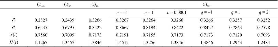
Using our results in Sections 3 and 4, the MLE esti-mates and the Bayes estiesti-mates of , , ( ) S t and ( )H t have been computed and the results are displayed in Ta-ble 3. By using (18) the 95% approximate confidence interval of and are, respectively (–0.3148, 0.8027) and (–0.3958, 1.7547).
6. Simulation Study
Since the performance of the different methods cannot be compared theoretically, we perform Monte Carlo simula-
Table 1. Randomly grouped set
1 2 3 4 5 6
s using data from Stablein (1981).
7 8 9 10 11 12 0.197 0.534 0.115 0.296 0.121 0.466 0.529 1.447 0.863 0.132 0.395 0.696 2.825 3.658 3.978 3.743 2.343 2.178
13 14 15 16 17 18 0.26 1.099 0.501 0.458 0.641 0.334
0.54 4.003 1.553 1.485 2.83 2.416 19 20 21 22 23 0.57 0.164 0.203 0.282 0.047
[image:6.595.55.540.524.605.2]1.271 1.589 1.326 0.841 2.444 0.644 1.219 0.507 3.578 1.581 4.033
Table 2. Prior i yper parameter values and the posterior probab es.
7
nformation, h iliti
j 1 2 3 4 5 6 8 9 10
j
0.25 0.26 0.27 28 0.29 0.30 0.31 0.32 0.0. 33 0.34
j
e 0.1 0.1 0.1 .1 0.1 0.1 0.1 0. 0.
3 340 0.339 0.338 0.336 0. 0.334 0.078 0.075 0.072 0.069 0.066 0.064 0.062 0.059 0.057 0.056
0 1 0.1 1
j
a 0.346 0.344 0.34 0.341 0. 335
j
b
j
p 0.0021 0.0041 0.0078 0.0148 0.0280 0.0482 0.0822 0.1543 0.2613 0.3973
S
Table 3. The ML and the Bayes estimates of , , ( )t andH t( )witht= 0.4.
(.)ML (.)BS (.)BL (.)GE
c = –1 c = 1 c = 0. 01 00 q=1 = 1 q q= 2
0.2827 0.2439 0.3266 3267 .3264 0.3266 0.3266 0.3257 0.3252 0. 0
0.6235 5 22 667 8194 0.8422 0.8422 0.7863
0.7560 0.7099 0.7173 0.7191 0.7155 0.7173 0.7173 0.7120 0.7093
0.679 0.84 0.8 0. 0.7578
( )
S t
( )
[image:6.595.57.539.637.719.2]T. A. ABUSHAL 167
tions to compare th performa ces of the ifferent esti- mators for different sampling schemes. All the co -
tions a perfo ith ium
Mathematica 8 used different size
number f gro er p s d
effective p ( nd diffe sam
hemes (i.e., es).W wo
e n d
mputa re rmed w a Pent IV processor using
.0. We sample s ( =n
t o ups), diff ent grou izes (k),
nt t
ifferen sam le sizes
different
m), a valu
re e used
pling sets of
sc Ri
parameter values: = 1, = 0.5 and = 0.1, = 0.2, mainly to compare the MLEs and different Bayes estimators in terms of their mean squared errors (MSEs), and also to explore their effects on different parame values.
To generate progressive st- failure censored samples from CRD, we used the a orithm proposed by [13], with the fact that, the pro
, , , 2; , , , , ; , ,
R R R
m n k X m n k Xm m n k with distribution function ( )
ter fir
lg
gressive first-failure censored sample
1;
X
F x , can be viewed as a progressive type II censored sample from a population with distribution function 1 (1 ( ))k
F x . We assume pu
censoring scheme, only from
the following
that the number of items
e II:
tting in a life test is (n k ) items, where n denotes the number of groups and k denotes the number of items in each group. Using a progressive first-failure m observations are record the test. To compare the performances of the esti-mation procedures developed in this paper, we consider
three progressive censoring schemes ( .C S ), namely:
Scheme I: Rm=nm, Ri=0 for im.
Schem R1=n m , Ri= 0 for i1. Scheme III: 1
2
= m
R nm, Ri = 0 for
1 m
i
2
, and
; if
m odd 2
2
= m
R n m , Ri= 0 for
2 2 m i n.
thr oring schemes ar spon
spectively, to the cases of all s g i s are re-moved from ent at the last failure point, first
fa midpoint. Also, it sh e noted
scheme I is the Type-II first-failure censored scheme. -7, we repo the m uared er (MSEs) of the ML estimates and different Bayes esti-m
; if m eve
The ee cens e corre ding,
re-urvivin tem the experim
ilure point and ould b that
In Tables 4 rt ean sq rors
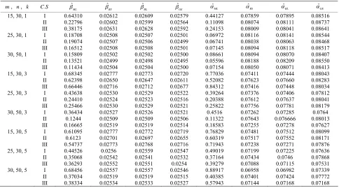
ates of the parameters, reliability and hazard rate func-tions, based on 1000 replications. The results are re-ported in Tables 4 and 5 for the parameters values
( = 1, = 0.5) . Tables 6 and 7 display the same results for the parameters values ( = 0.1, = 0.2).
7. Conclusions
In this paper, the maximum likelihood and Bayes meth-ods are used for estimating parameters, reliability func-rate function of the CRD based on a new
censoring scheme, called -fa
tion and hazard
a progressive first ilure cen-oring scheme. Combining the concept of first-failure
concept of progressive censoring, a
bl
s
censoring and the
Ta e 4. MSEs of estimates of andwhen ( = 1,= 0.5;c=q= 1).
m, n, k C S. ˆML
ˆ
BS
ˆ
BL
ˆ
GE
ˆML ˆBS ˆBL ˆGE 15, 30, 1 I 4.6722 0.1581 0.1121 0.1580 0.4997 0.2319 0.2024 0.1801
II 3.0944 0.1561 0.1109 3.2318 0.1574 0.1117 I 2.03 0.1596 0.1130
II 1.6751 0.1595 0.1129 0.1594 0.0812 0.1323 0.1219 0.1107
III 5 0.0819 0.1406 0.1296 0.1181
30, 50, 1 I 1132 0.1599 0.2759 0.1528 0.1429 0.1323 II 1.1589 0.1598 0.1131 0.1598 0.0401 0.1187 0.1109 0.1020 III 1.1757 0.1599 0.1132 0.1599 0.0851 0.1361 0.1272 0.1173 0.1558 0.1440 0.1744 0.1522 0.1334 0.1572 0.3022 0.2199 0.1919 0.1702 0.1596 0.1032 0.1341 0.1236 0.1123 III
25, 30, 1 00
1.7901 0.1596 0.1129 0.159 3.4690 0.1599 0.
Table 5. MSEs of estimates ofS t( )andH t( )when (= 1,= 0.5; c =q=1andt= 1.5).
m, n, k C S. SˆML
ˆ
BS
S SˆBL
ˆ
G
SE
ˆ
ML
H HˆBS
ˆ
BL
H HˆGE
15, 30, 1 I 0.0082 0.0217 0.0226 0.0275 0.0414 0.1260 .1113 0.0958 0
II 0.0211 0.0220 0.0928 0.0819 0.0696
III 0.0085 0.0206 0.0215 0.0262 0.0343 0.1190 0.1051 0.0902
25, 30, 1 I 0.006 0.012 0.0134 0.0153 0.0123 0. 0
II 0.0151 0.0113 0.0656 0.0607 0.0537
0.0127 0.07 0.0654 0.0581
30, 50, 1 0. 0767 0.0719 0.0651
II 0.0066 0.0114 0.0118 0.0132 0.0094 0.0578 0.0542 0.0487 III 0.0046 0.0133 0.0137 0.0154 0.0114 0.0672 0.063 0.0567
0
0.0118 0.0165 0.0172
2 9 0665 .0616 0.0544
0.0074 0.0127 0.0131
III 0.0067 0.0137 0.0141 0.0162 06
I 0.0043 0.0152 0156 0.0175 0.0202 0.
15, 30, 3 I 0.0087 0.0239 0.0250 0.0305 0.0598 0.1375 0.1216 0.1044
II 0.0076 0.0218 0.0227 0.0277 0.0406 0.1303 0.1148 0.0994 III 0.0077 0.0244 0.0254 0.031 0.0514 0.1453 0.1281 0.1111
25, 30, 3 I 0.0048 0.0197 0.0203 0.0231 0.0364 0.1030 0.0955 0.0858
II 0.0046 0.0174 0.018 0.0205 0.0289 0.0901 0.0835 0.0747
III 0.0053 0.0195 0.02 0.0228 0.0336 0.1035 0.096 0.0866
30, 50, 3 I 0.0056 0.0227 0.0233 0.0259 0.044 0.1166 0.1095 0.1005
II 0.0039 0.0168 0.0173 0.0194 0.0234 0.085 0.0798 0.724 III 0.0048 0.0189 0.0194 0.0217 0.0372 0.0970 0.0911 0.0831
15, 30, 5 I 0.0113 0.0272 0.0283 0.0344 0.0687 0.1587 0.1403 0.1216
II 0.0083 0.0245 0.0256 0.0312 0.0586 0.1464 0.1291 0.112 III 0.0086 0.0245 0.0255 0.0311 0.0563 0.1416 0.1252 0.1079
25, 30, 5 I 0.0063 0.0217 0.0223 0.0254 0.0468 0.1153 0.1069 0.0967
II 0.0056 0.0209 0.0215 0.0245 0.0464 0.1096 0.1017 0.0916
III 0.0052 0.0202 .0208 0.0236 0.0401 0.1050 0.0974 0.0875
30, 50, 5 I 0.0066 0.0214 0.0220 0.0245 0.0504 0.1082 0.1016 0.0928
[image:8.595.54.539.106.375.2]II 0.0046 0.0191 0.0196 0.0219 0.0368 0.0968 0.0909 0.0828 III 0.0058 0.0208 0.0214 0.0238 0.0480 0.1060 0.0996 0.0911
Table 6. MSEs of estimates andwith ( = 0.1,= 0.2; =c q= 1).
m, n, k C S. ˆML ˆBS ˆBL ˆGE ˆML ˆBS ˆBL ˆGE
15, 30, 1 I 0.64310 0.02612 0.02609 0.02579 .44127 .07859 .07895 0.08516 0 0 0
II 0.2 0.0 0.0 0. 0 0 0
II 0.38175 0.02631 0.02628 0.02592 0. 0 0
25, 30, 1 I 0.1 0.0 0.0 0. 0 0 0
II 0.19074 0.02507 0.02506 0.02499 0.06741 0.08038 0.08063 0.08468
III 0.16 8 0 0 145 0.08094 0.08118 0.08517
30, 50, 1 I 0.1580 2 0.0250 1 0.08094 0.08070 0.08407
II 0.1352 0.02499 0.02498 0.0249 6 0.08188 0.08209 0.08550
III 0.11434 0.02504 0.02504 0.02500 0.07154 0.08050 0.08071 0.08413
2796 2602 2599 02564 .11098 .08074 .08111 0.08737
I 24153 .08009 .08041 0.08641
8708 2508 2507 02501 .06972 .08116 .08141 0.08544
512 0.02508 0.0250 .02501 .07
9 0.02502 0.0250 0 0.0866
1 5 0.0559
15, 30, 3 I 0.68345 0.02777 0.02773 0.02720 0.77036 0.07411 0.07444 0.08043
II 0.62398 0.02650 0.02647 0.02611 0.52082 0.07623 0.07660 0.08283
III 0.66446 0.02716 0.02712 0.02677 0.84312 0.07416 0.07448 0.08034
25, 30, 3 I 0.43638 0.02530 0.02529 0.02522 0.39264 0.07376 0.07406 0.07812
II 0.24410 0.02524 0.02523 0.02516 0.20388 0.07612 0.07637 0.08041
III 0.25466 0.02530 0.02529 0.02521 0.25822 0.07756 0.07781 0.08179
30, 50, 3 I 0.36434 0.02527 0.02526 0.02521 0.4516 0.07262 0.07285 0.0764
II 0.1244 0.02509 0.02509 0.02506 0.11322 0.07643 0.076666 0.08013
III 0.16665 0.02519 0.02519 0.02514 0.18583 0.07255 0.07278 0.07627
15, 30, 5 I 0.61095 0.02777 0.02772 0.02719 0.76829 0.07481 0.07512 0.08099
II 0.6123 0.02701 0.02697 0.02655 0.60319 0.07517 0.07552 0.08171
III 0.54737 0.02773 0.02768 0.02716 0.71943 0.07238 0.07271 0.07876
25, 30, 5 I 0.44526 0.0256 0.02559 0.02547 0.49019 0.07199 0.07225 0.07636
II 0.35068 0.02542 0.02541 0.02532 0.37164 0.07434 0.0746 0.07868
III 0.36293 0.02552 0.02551 0.0254 0.39279 0.07088 0.07115 0.07531
30, 50, 5 I 0.68456 0.02557 0.02557 0.02546 0.88917 0.06958 0.06982 0.07339
II 0.37034 0.02519 0.02519 0.02515 0.40385 0.07401 0.07424 0.07772
III 0.38334 0.02534 0.02533 0.02527 0.57943 0.07144 0.07168 0.07168
progressive fi ailu ring has n-
tro y [2 Thi ing sc has a es
in terms of reducing , in ore re
ut o rst-f re censo scheme been i
duced b 1]. s censor heme dvantag
test time which m items a
used b nly m of (n k ) items res.
ew c h e pre er s w
ings can be rou anag a
are failu Based on this n ensoring sc eme, th sent pap hows ho the th
[image:8.595.56.540.403.672.2]T. A. ABUSHAL 169
able of es
T 7. MSEs timates ofS t and( ) H t when (( ) = 0.1,= 0.2; =c q= 1andt= 1.5 ).
m, n, k C S. SˆML
ˆ
BS
S SˆBL
ˆ
GE
S HˆML HˆBS HˆBL HˆGE
15, 30, 1 I 0.104547 0.17122 0.16955 0.16638 0.24275 0.10171 0.1023 0.1101
II 0.0966954 0.17595 0.17429
III 0.0996995 0.17337 0.17174
25, 30, 1 I 0.07744 0.1756 0.17453
0 64 0.104
0 0
III 0. 07716 0.10407 0.10516 0.11015
30, 50, 1 3 3 0.08715 0.1042 0.10877
II 0.07092 0.17664 0.17573 0.17403 0.06067 0.10601 0.10634 0.11059
III 0.06447 0.17376 0.17285 0.17112 0.07603 0.10425 0.10459 0.10886
25, 30, 3
0
.17113 0.10 9 46 0.10506 0.11292
.16872 0.1746 0.10357 0.1041 0.11165 0.1725 0.07316 0.10507 0.10547 0.11049
II 0.08063 0.17389 0.17281 .17076 0.06942 0.10407 0.10448 0.10953
0.07749 0.17502 17396 0.17195 0.
I 0.06926 0.17383 0.1729 0.1712 2 0.10455
15, 30, 3 I
II 0.1600.11215 69 0.1610.16632 55 0.159 0.16464 89 0.1560.1614 75 0.48559 0.096 0.09650.27853 0.09873 0.09932 4 0.1041 0.10716
III 0.1446 0.16122 0.15959 0.15652 0.47758 0.096 0.09653 0.10394
I 0.10164 0.16041 0.15929 0.15712 0.23557 0.09566 0.09609 0.1012
II 0.08286 0.16497 0.16387 0.16176 0.15397 0.09864 0.09906 0.10411
III 0.09343 0.16806 0.16699 0.16493 0.19534 0.10047 0.10087 0.10585
30, 50, 3 I 0.12342 0.1577 0.15673 0.15483 0.32138 0.09427 0.09496 0.09906
II 0.07157 0.1655 0.16456 0.16275 0.11354 0.09909 0.09945 0.10379
III 0.09084 0.15749 0.15653 0.15465 0.17242 0.09415 0.09452 0.09888
15, 30, 5 I 0.015722 0.16256 0.16092 0.15786 0.47972 0.09686 0.09737 0.1048
II 0.01313 0.16406 0.16237 0.15913 0.36439 0
0.0938 .09738 0.09796 0.10574
III 0.015951 0.15781 0.15612 0.15291 0.47296 0.09436 0.10198
25, 30, 5 I .013146 0.15666 0.15553 0.15332 0.3405 0
0.0964
.09342 0.09385 0.09899
II 0.10276 0.16138 0.16026 0.1581 0.23814 0.09682 0.10193
III 0.11713 0.15424 0.15309 0.15082 0.27399 0.09202 0.09246 0.09766
30, 50, 5 I 0.1593 0.15165 0.15066 0.14871 0.49866 0.09042 0.09081 0.09526
II 0.10173 0.16047 0.15951 0.15766 0.24817 0.09601 0.09638 0.10073
III 0.11933 0.15529 0.15432 0.15241 0.32279 0.09276 0.09314 0.9754
Bayesian and sical rks. e co
the m ximum eliho and stim
th ters of the C ell a urvi
param ters, re ility ard ction
pr ely f st-failu ored e B
timators are discussed mme asy
ss f ns. e use crete trib
clas framewo We hav nsidered
a lik od (ML) Bayes e ates for
e parame RD, as w s some s val time
e liab and haz rate fun s using
ogressiv ir re cens data. Th ayes
es-under sy tric and mmetric lo unctio Th of a dis prior dis ution for parameter resulted in a closed form expression for the posterior pdf, and the equal probabilities in the dis-crete distribution cased an element of uncertainly, which can be desirable in some cases. All of the results ob-tained in this article can be specialized to: a): the first- failure censored data when R= {0,0, ,0} . b): the pro- gressive type II censored order statistics if = 1k . c): Type II censored order statistics when = 1k and
= {0,0, ,nm}
R . d): the complete sample case when
= 1
k and R= {0,0, ,0} . A simulation study was
conducted to examine the performance of the different estimators. From the results, we observe the following:
The Bayes estimates are better than the MLEs in general, and the Bayes estimates relative to asym-metric loss functions (LINEX and GE l per-formed better than the others in the sense of com-ng t E of the estimates. This was true for all censored schemes.
From all Tables, as the effective sample proportion /m n increases, the MSE of the estimators, reduc oss) pari he MS
ring or a an e
n d ing s is
ost t; n
at t (all
rst f ith
e ot s e of s.
o ac e s he
e significantly. Concerning a progressive type-II cen-
asymmetric loss functions c and q, we examine different values of c and q we see that if c is near to 0, and q= 1
so scheme (k the for f sc e p in t effe
= 1), f fixed m (R
l em
n m
d n, w
ca etermine censor cheme )
es
g th et
, which m efficien example, in all tab it is see th he case o heme II items r oved at the
is better than fi ailure tim oint), w ( = 1)k
th her case he sens compari e MSE
T cess the ct of th hape para ers of t , then the Bayes estimates are almost the same as the estimates under SEL, see Table 3. This is one of the useful properties of working with the asymmetric loss functions.
The results establish that for optimum decision making, important should be given on the choice of loss function and not just the choice of prior distri-bution only.
The simulation study shows that the MSEs for all estimates are increases as the value of the shape and scale parameters increases.8. References
[1] R. Viveros and N. Balakrishnan, “Interval Estimation of Pa- rameters of Life from Progressively Censored Data,”
Te- chnometrics, Vol. 36, No. 1, 1994, pp. 84-91.
doi:10.2307/1269201
[image:9.595.58.539.106.373.2]I Cen-Algorithm for Generating Progressively Type-I sored Samples,” TheAmerican Statistician, Vol. 49, No.
2, 1995, pp. 229-230.doi:10.2307/2684646
[3] N. Balakrishnan and R. A. Sandhu, “Best Linear Unbi-ased and Maximum Likelihood Estimation for Exponen-tial Distributions under General Progressive Type-II Cen-sored Samples,” Sankhya: The Indian Journal of Seri-estics, Vol. 58, No. 1, 1996, pp. 1-9.
] P. Mostert, J. Roux and A. Bek
[4 ker, “Bayes Estimators of Using the Compound Ray
al of South African Statistical Association,
Vol. 33, No. 2 ,1999, pp. 117-138.
ns on
. 2, 2000, pp. 199-203. the Life Time Parameters
model,” Journ
leigh
[5] U. Balasooriya and N. Balakrishnan, “Reliability Sam-pling Plans for Log-Normal Distribution Based on Pro-gressively Censored Samples,” IEEE Transactio Reliability, Vol. 49, No
doi:10.1109/24.877338
[6] A. Bekker, J. Roux and P. Mostert, “A Generalization of the Compound Rayleigh Distribution: Using a Bayesian Methods on Cancer Survival Times,” Communications in Statistics—Theory and Methods, Vol. 29, No. 7, 2000, pp.
1419-1433.doi:10.1080/03610920008832554
[7] H. K. T. Ng, P. S. Chan and N. Balakrishnan, “Optimal Progressive Censoring Plans for the Weibull Distribu- tion,” Technometrics, Vol. 46, No. 4, 2004, pp. 470-481.
doi:10.1198/004017004000000482
[8] H. K. T. Ng, “Parameter estimation for a modifiied Wei- bull Distribution, for Progressively Type-II Censored Samples,” IEEE TransactionsReliability, Vol. 54, No. 3,
2005, pp. 374-380.doi:10.1109/TR.2005.853036
[9] N. Balakrishnan, N. Kannan, C. T. Lin and H. K. T. Ng, “Point and Interval Estimation for Gaussian Distribution Based on Progressively Type-II Censored
IEEE Transactions on R
Samples,”
eliability, Vol. 52, No. 1, 2003,
pp. 90-95.doi:10.1109/TR.2002.805786
[10] A. A. Soliman,“Estimation of Parameters of Life from Progressively Censored Data Using Burr-XII Model,”
IEEE TransactionsReliability, Vol. 54, No. 1, 2005, pp. 34-42.doi:10.1109/TR.2004.842528
[11] A. A. Soliman, “Estimation for Pareto Model Using Gen-eral Progressive Censored Data and Asymmetric Loss,”
Communications in Statistics—Theory and Methods, Vol.
37, No. 9, 2008, pp. 1353-1370.
doi:10.1080/03610920701825957
[12] D. G. Chen and Y. L. Lio, “Parameter Estimations for Generalized Exponential Distribution under Progressive Type-I Interval Censoring,” Computational Statistics and Data Analysis, Vol.54, No. 6, 2010, pp. 1581-1591.
doi:10.1016/j.csda.2010.01.007
[13] N. Balakrishnan and R. Aggarwala, “Progressive Cen-soring—Theory, Methods and Applications,” Birkhäuser, Boston, 2000.
[14] N. Balakrishnan, “Progressive Censoring Methodology: An Appraisal,” Test, Vol. 16, No. 2007, pp. 211-289.
doi:10.1007/s11749-007-0061-y
[15] L. G. Johnson, “Theory and Technique of Variation
sactions on Reliability,
Re-search,” Elsevier, Amsterdam, 1964.
[16] C.-H. Jun, S. Balamurali and S.-H. Lee, “Variables Sam-pling Plans for Weibull Distributed Lifetimes under Sud-den Death Testing,” IEEE Tran
Vol. 55, No. 1, 2006, pp. 53-58.
doi:10.1109/TR.2005.863802
[17] J.-W. Wu, W.-L. Hung and C.-H. Tsai, “Estimation of the Parameters of the Gompertz Distribution under the First Failure-Censored Sampling Plan,” Statistics, Vol. 37,
6, 2003, pp. 517-525.
No.
doi:10.1080/02331880310001598864
[18] J.-W. Wu and H. -Y. Yu, “Statistical Inference about the Shape Parameter of the Burr Type XII Distribution under the Failure-Censored Sampling Plan,” Applied Mathe-matics and computation, Vol. 163, No. 1, 2005, pp. 443- 482.doi:10.1016/j.amc.2004.02.019
[19] J.-W. Wu, T.-R. Tsai and L.-Y. Ouyang, “Limited Fail- ure-Censored Life Test for the Weibull Distribution,”
IEEE Transactions on Reliability, Vol. 50, No. 1, 2001,
pp. 107-111.doi:10.1109/24.935024
[20] W.-C. Lee, L.-W. Wu and H.-Y. Yu, “Statistical Infer-ence about the Shape Parameter of the Bathtub-Shaped Distribution under the Failure-Censored Sampling Plan,”
, 2009, pp.
, “Bayesian
Predic-lanning and International Journal of Information and Management Sciences, Vol. 18, No. 2, 2007, pp. 157-172.
[21] S.-J. Wu and C. Kus, “On Estimation Based on Progres-sive First Failure-Censored Sampling,” Computational Statistics and Data Analysis, Vol. 53, No. 10
1-12.
[22] E. K. AL-Hussaini and Z. F. Jaheen, “Bayes Estimation of the Parameters, Reliability and Failure Rate Functions of the Burr Type XII Failure Model,” Journal of Statistics Computation and Simulation, Vol. 44, 1992, pp. 31-40. [23] E. K. AL-Hussaini and Z. F. Jaheen, “Approximate Bayes
Estimators Applied to the Burr Model,” Communications in Statistics, Vol. 23, 1994, pp. 99-121.
[24] E. K. AL-Hussaini and Z. F. Jaheen
tion Bounds for the Burr XII Model,” Communications in Statistics, Vol. 24, 1995, pp. 1829-1842.
[25] E. K. AL-Hussaini and Z. F. Jaheen, “Bayesian Predic-tion Bounds for the Burr Type XII DistribuPredic-tion in the Presence of Outliers,” Journal of Statistical P
Inference, Vol. 55, No. 1, 1996, pp. 23-37.
doi:10.1016/0378-3758(95)00184-0
[26] E. K. AL-Hussaini, “Predicting Observables from a Gen-eral Class of Distributions,” Journal of Statistical Plan-ning and Inference, Vol. 79, No. 1, 1999, pp. 79-91.
doi:10.1016/S0378-3758(98)00228-6
[27] N. Balakrishnan and M. Kateri, “Statistical Evidence in Contingency Tables Analysis,” Journal of Statistical Pla- nning and Inference, Vol. 138, No. 4, 2008, pp. 873- 887.
doi:10.1016/j.jspi.2007.02.005
[28] H. R. Varian, “A Bayesian Approach to Real State As-sessment,” In: E. F. Stephen and A. Zellner, Eds., Studies in Bayesian Econometrics and Statistics in Honor of Leo-nard J. Savage, North-Holland, Amsterdam, 1975, pp.
195-208.
T. A. ABUSHAL 171
Vol. 73,
atcom.2006.05.002
Estimators of Reliability Performances Using LINEX loss under Progressively Type-II Censored Samples,”
Mathematics and Computers in Simulation,
5, 2007, pp. 320-326.
No.
doi:10.1016/j.m
7.07.002
[30] G. Prakash and D. C. Singh, “Shrinkage Estimation in Exponential Type-II Censored Data under LINEX Loss,”
Journal of the Korean Statistical Society, Vol. 37, No
2008, pp. 53-61.
. 1,
doi:10.1016/j.jkss.200
(86)90108-4
[31] D. K. Day, M. Ghosh and C. Srinivasan, “Simultaneous Estimation of Parameters under Entropy Loss,” Journal of Statistical Planning and Inference, Vol. 52, 1987, pp.
347-363.doi:10.1016/0378-3758
[32] D. K. Day and P. L. Liu, “On Comparison of Estimation in Generalized Life Model,” Microelectronics Reliability,
Vol. 32, No. 1-2, 1992, pp. 207-221.
doi:10.1016/0026-2714(92)90099-7
[33] R. M. Soland, “Bayesian analysis of the Weibull Process with Unknown Scale and Shape Parameters,” IEEE Transactions on Reliability, Vol. 18, No. 4, 1969, pp.
181-184.doi:10.1109/TR.1969.5216348
[34] A. A. Soliman, A. H. Abd Ellah and K. S. Sultan, “Com-parison of Estimates Using Record Statistics from Wei- bull Model: Bayesian and Non-Bayesian Approaches,”
Computational Statistics & Data Analysis, Vol. 51, No. 3,
2006, pp. 2065-2077.
doi:10.1016/j.csda.2005.12.020
[35] H. F. Martz and R. A. Waller, “Bayesian Reliability Ana- lysis,” Wiley, New York, 1982.
[36] D. M. Stablein, W. H. Carter and J. W. Novak, “Analysis of Survival Data with Non-Proportional Hazard Func-tions,” Controlled Clinical Trials, Vol. 2, No. 2, 1981, pp.