Munich Personal RePEc Archive
On various confidence intervals
post-model-selection
Leeb, Hannes and Pötscher, Benedikt M. and Ewald, Karl
University of Vienna, University of Vienna, University of Technology
Vienna
2014
Online at
https://mpra.ub.uni-muenchen.de/58326/
On various confidence intervals
post-model-selection
Hannes Leeb
1, Benedikt M. P¨
otscher
1, and Karl Ewald
21
University of Vienna
2Vienna University of Technology
First version: January 2014
This version: August 2014
Abstract
We compare several confidence intervals after model selection in the setting recently studied by Berk et al. (2013), where the goal is to cover not the true parameter but a certain non-standard quantity of interest that depends on the selected model. In particular, we compare the PoSI-intervals that are proposed in that reference with the ‘naive’ confidence interval, which is constructed as if the selected model were correct and fixed a-priori (thus ignoring the presence of model selection). Overall, we find that the actual coverage probabilities of all these intervals deviate only moderately from the desired nominal coverage probability. This finding is in stark contrast to several papers in the existing literature, where the goal is to cover the true parameter.
1
Introduction and Overview
There is ample evidence in the literature that model selection can have a detri-mental impact on subsequently constructed inference procedures like confidence sets, if these are constructed in the ‘naive’ way where the presence of model selection is ignored. Such results are reported, for example, by Brown (1967); Buehler and Feddersen (1963); Dijkstra and Veldkamp (1988); Kabaila (1998, 2009); Kabaila and Leeb (2006); Leeb (2006); Leeb and P¨otscher (2003, 2005, 2006a,b, 2008a,b); Olshen (1973); P¨otscher (1991, 2006); P¨otscher and Leeb (2009); P¨otscher and Schneider (2009, 2010, 2011); Sen (1979); Sen and Saleh (1987).
in that they consider confidence intervals fora different quantity of interest: In the aforementioned analyses, the quantity of interest (the coverage target) is always a fixed parameter or sub-parameter of the data-generating model. In Berk et al. (2013), on the other hand, a different and non-standard coverage target is considered that depends on the selected model. [Even if an overall correct model is assumed, that non-standard coverage target doesnotcoincide with a parameter in the model, except for degenerate and trivial situations.] By design, the PoSI-intervals hence do not provide a solution to the more traditional problem, where the goal is to cover a parameter in the overall model after model selection.
Berk et al. (2013) motivate the need for PoSI-intervals by the poor perfor-mance of the ‘naive’ interval as observed in the studies mentioned in the first paragraph of this section. However, these studies donotdeal with the perfor-mance of the ‘naive’ procedures post-model-selection when the coverage target is as in Berk et al. (2013). This raises the question of how the ‘naive’ interval performs when it is used to cover the coverage target considered in Berk et al. (2013). The main contribution of this paper is to answer this. In particular, we compare ‘naive’ confidence intervals and PoSI-intervals in the setting of Berk et al. (2013). [The results in the present paper are partly based on Ewald (2012), and we refer to this thesis for additional results and discussion.]
We find that the minimal coverage probability of the ‘naive’ interval is slightly below the nominal one, while that of the various PoSI intervals is slightly above, when the coverage target is as in Berk et al. (2013) and when AIC, BIC, or the LASSO are used for model selection. In the scenarios that we consider, the coverage probabilities of all these intervals are mostly within 10% of the nominal coverage probability. In the more traditional setting where the cov-erage target is a parameter in the overall model, however, all these intervals generally fail to deliver the desired minimal coverage probability. [Note that the various PoSI-intervals are not designed to deal with this coverage target.] For example, consider the scenario depicted by the solid curves in Figure 1 on page 10: There, a ‘naive’ confidence interval post-model-selection with nominal coverage probability 0.95 has a minimal coverage probability of about 0.91 and the corresponding PoSI-interval has a minimal coverage probability of about 0.96, if the coverage target is as in Berk et al. (2013). But if the coverage target is a parameter in the overall model, the minimal coverage probabilities of the ‘naive’ interval and of the PoSI-interval drop to about 0.56 and 0.62, respectively.
sce-narios; the first scenario is also studied by Kabaila and Leeb (2006), and the other two scenarios are taken from Berk et al. (2013). [The code used for the computations in Section 3 and for the simulations in Section 4 is available from the first author on request.] Finally, in the Appendix we present an example with a coverage target that is similar to, but slightly different from, that con-sidered in Berk et al. (2013). The interesting feature of this example is that the ‘naive’ confidence interval here is valid, in the sense that its coverage probability is never below the nominal level.
2
Coverage Targets and Confidence Intervals
Throughout, we consider a set ofn homoskedastic Gaussian observations with mean vectorµ∈Rn and common varianceσ2>0, i.e.,
y = µ+u, (2.1)
whereu∼N(0, σ2I
n). We further assume that we have an estimator ˆσ2 forσ2
that is independent of all the least-squares estimators that will be introduced shortly. See Remark 2.1(ii) for some cautionary comments regarding our as-sumptions on ˆσ2. For the estimator ˆσ2, we either assume that it is distributed as a chi-squared random variable withrdegrees of freedom multiplied byσ2/r, i.e., ˆσ2
∼ σ2χ2
r/r, for some r ≥ 1; or we assume that the variance is known
a-priori, in which case we set ˆσ2 = σ2 and r =
∞. Unless noted otherwise, all considerations that follow apply to both the known-variance case and the unknown-variance case. The joint distribution of y and ˆσ depends on the pa-rametersµ∈Rn andσ >0, and will be denoted by Pµ,σ.
The available explanatory variables are represented by the columns of a fixedn×pmatrixX, where we allow forp > n; again, see Remark 2.1(ii). We consider models wherey is regressed on a (non-empty) subset of the regressors inX: For each modelM ⊆ {1, . . . , p}withM 6=∅, writeXM for the matrix of
those columns ofX whose indices lie inM. WritingM asM ={j1, . . . , j|M|} ⊆
{1, . . . , p}, we thus have XM = (Xj1, . . . , Xj|M|), where Xj denotes the j-th
column of X, and where |M| denotes the size of M. Write M for a user-specified (non-empty) collection of candidate models. Throughout, we assume thatMconsists only of submodels of full column rank, i.e., we assume that the rank ofXM equals|M| and satisfies 1≤ |M| ≤nfor eachM ∈ M.
Under a candidate modelM ∈ M,y is modeled as
y = XMβM +vM,
where βM corresponds to the orthogonal projection of µ from (2.1) onto the
column-space of XM, i.e., βM = (XM′ XM)−1XM′ µ. The least-squares
esti-mator corresponding to the model M will be denoted by ˆβM, i.e., ˆβM =
(X′
MXM)−1XM′ y. The working model M is correct if XMβM = µ; in that
case, we have vM = u. Otherwise, i.e., if XMβM 6=µ, the working model is
incorrect, and we havevM =µ−XMβM+u. Irrespective of whether the
particular, ˆβM is an unbiased estimator for βM, irrespective of whether or not
the modelM is correct. As noted earlier, we assume that the variance estimator ˆ
σ2is independent of the collection of estimators ˆβ
M forM ∈ M.
To pinpoint the regression coefficient of a given regressor Xj in a modelM
it appears in, we writeβj·M for that component ofβM that corresponds to the
regressorXj for eachj ∈M. Similarly, the components of ˆβM are indexed as
ˆ
βj·M for j ∈M. This convention is called ‘full model indexing’ in Berk et al.
(2013).
Consider now a model selection procedure, i.e., a data-driven rule that selects a model ˆM ∈ Mfrom the poolMof candidate models, and the resulting post-model-selection estimator ˆβMˆ. The coverage target considered in Berk et al. (2013) isβMˆ, or components thereof. Note that this coverage target is random, because it depends on the outcome of the model selection procedure.
Remark 2.1. (i) At least one author of the present paper believes that the merits ofβMˆ as a coverage target for inference are debatable: For example, the meaning of the first coefficient ofβMˆ depends on the selected model and hence also on the training data (y, X); the same applies to the dimension ofβMˆ. In particular, we stress that different model selection procedures (e.g., AIC, BIC, the LASSO, etc.) lead to different targetsβMˆ. We refer to Berk et al. (2013) for further discussion and motivation for studyingβMˆ. These authors make the case forβMˆ by arguing that the relevant setting is one where no correct overall model is available; however, in this situation the subsequent remark becomes especially important.
(ii) While the model (2.1) is non-parametric, the distributional requirements on ˆσ2 obviously are rather restrictive. However, these are the assumptions underlying the analysis in Berk et al. (2013), and we adopt them here in order to be in line with that reference. A leading case where these requirements are fulfilled is when (2.1) is replaced by theparametricmodely=Xβ+u, whenX
is as before and is assumed to be of full column rankp < n, and when ˆσ2 is the usual unbiased variance estimator in that model andr is set ton−p. In this leading case, however, the true parameterβin the overall model is well-defined and will then typically be the prime target of statistical inference, rather than the non-standard coverage target introduced in Berk et al. (2013). Outside of the parametric model just discussed, the requirements on ˆσ2 made in Berk et al. (2013), and also here, will only be satisfied in certain special cases, some of which are discussed at the end of Section 2.2 in Berk et al. (2013). [The requirements on ˆσ2 are also fulfilled (with r=n
−q), if we would maintain a true parametric model y =Zθ+ufor some observed n×q matrixZ of rank
q < nthat contains X as a submatrix; however, in this case one is back to the leading case discussed above, after redefiningMappropriately.]
In this paper, we will mainly focus on confidence intervals for the coefficient of one particular regressor in the selected model. Without loss of generality, assume that X1 is the regressor of interest, and that the coverage target is
first regressorX1is contained in all candidate models under consideration, i.e., we assume that 1 ∈ M for each M ∈ M. We seek to construct confidence intervals forβ1·Mˆ that are of the form
ˆ
β1·Mˆ ±Kσˆ1·Mˆ
for some constant K > 0, with ˆσ2
1·M defined by ˆσ12·M = ˆσ2[(XM′ XM)−1]1,1, where [. . .]1,1denotes the first diagonal element of the indicated matrix. Here, we abuse notation and writea±bfor the interval [a−b, a+b]. For a given level 1−αwith 0< α <1, the constantK should be chosen such that the minimal coverage probability is at least 1−α, i.e., such that
inf
µ,σPµ,σ
β1·Mˆ ∈ βˆ1·Mˆ ±Kσˆ1·Mˆ
≥ 1−α. (2.2)
Because the distribution of ( ˆβ1·M −β1·M)/σˆ1·M is independent of unknown
parameters and also independent ofM, it follows, forfixedM, that a confidence interval forβ1·M with minimal coverage probability 1−αis given by the textbook
interval ˆβ1·M±KNσˆ1·M, whereKN is the (1−α/2)-quantile of the distribution of
( ˆβ1·M−β1·M)/ˆσ1·M – a standard normal distribution in the known-variance case
and a t-distribution with r degrees of freedom in the unknown-variance case. In view of this, it is tempting to consider, as a confidence interval forβ1·Mˆ, the interval ˆβ1·Mˆ ±KNσˆ1·Mˆ. Because this construction ignores the model selection
step and treats the selected model ˆM as fixed, we will call this the ‘naive’ confidence interval.
The PoSI-interval developed in Berk et al. (2013) is obtained by first con-structing simultaneous confidence intervals for the components ofβM that are
centered at the corresponding components of ˆβM, for eachM ∈ M, with
cov-erage probability 1−α: More formally, the PoSI-constant KP is the unique
solution to
inf
µ,σPµ,σ
βj·M ∈βˆj·M±KPσˆj·M : j ∈M, M ∈ M
= 1−α, (2.3)
where the quantities ˆσ2
j·M are defined like ˆσ21·M but with j replacing 1. By
construction, the PoSI-constantKP is such that we obtain simultaneous
confi-dence intervals for the components ofβMˆ that are centered at the corresponding components of ˆβMˆ. In other words, (2.3) implies
inf
µ,σPµ,σ
βj·Mˆ ∈βˆj·Mˆ ±KPσˆj·Mˆ : j∈Mˆ
≥ 1−α. (2.4)
In particular, (2.2) holds when KP replaces K. For computing the constant
KP, we note that the probability in (2.3) can also be written as Pµ,σ(|βˆj·M −
βj·M|/σˆj·M ≤KP : j∈M, M ∈ M). This probability is not hard to compute,
because it involves only the random variables ( ˆβj·M −βj·M)/σˆj·M, which are
only depending onX. In particular, the probability in (2.3) does not depend on
µor σ2. Similar considerations apply, mutatis mutandis, to the constant K
P1 that is introduced in the following paragraph.
A modification of the preceding procedure, which is also proposed in Berk et al. (2013), is useful when inference is focused on a particular component of βMˆ, instead of on all components. Recall that the coverage target in (2.2) is the first component of βMˆ, i.e., β1·Mˆ. The PoSI1-constant KP1 provides simultaneous confidence intervals forβ1·M centered at ˆβ1·M for each M ∈ M.
In particular,KP1 is the unique solution to
inf
µ,σPµ,σ
β1·M ∈βˆ1·M±KP1σˆ1·M : M ∈ M
= 1−α. (2.5)
Again by construction, (2.2) holds whenKP1replacesK.
Like the PoSI-constants discussed so far, other procedures for controlling the family-wise error rate can be used. Consider, for example, Scheff´e’s method: Recall that X denotes the matrix of all available explanatory variables, and note that ( ˆβj·M−βj·M) is a linear function ofY−µ, i.e., a function of the form
υ′(Y
−µ), for a certain vectorυ6= 0 in the span ofX. The Scheff´e constantKS
is chosen such that
Pµ,σ
sup
ν∈span(X)
ν6=0
ν′(Y
−µ) ˆ
σkνk ≤KS
= 1−α.
Then the relations (2.4) and, in particular, (2.2) hold whenKS replaces both
KandKP. Note that the probability in the preceding display does not depend
on µ and σ, and that the constant KS is easily computed as follows: Let s
denote the rank of X. In the known-variance case, KS is the square root of
the (1−α)-quantile of a chi-square distribution withs degrees of freedom. In the unknown-variance case,KS is the square root of the product of s and the
(1−α)-quantile of anF-distribution withsandrdegrees of freedom.
Using the constants KP, KP1 or KS gives valid confidence intervals
post-model-selection, i.e., intervals that satisfy (2.2), because these constants give simultaneous confidence intervals for all quantities of interest that can occur; for example, (2.4) follows from (2.3), which in turn guarantees that (2.2) holds when KP replaces K. One advantage of this is that a coverage probability
of at least 1−α is guaranteed, irrespective of the model selection procedure ˆ
M (as long as it takes values inM). In particular, this is guaranteed even if the model is selected by statistically inane methods like the SPAR-procedure mentioned in Section 4.9 of Berk et al. (2013). The price for this is that the PoSI constantsKP andKP1 may be overly conservative for aparticularmodel selection procedure ˆM. [In this context, we note that equality holds in (2.4) for the SPAR-procedure, and that equality holds in (2.2) for a variant of the SPAR-procedure which selects that model ˆM which maximizes|βˆ1·M|/σˆ1·M over
Lastly, we will also consider the obvious approach where one chooses the smallest constantKsuch that (2.2) is satisfied. We will denote this constant by
K∗ (provided it exists). This is, of course, a well-known standard construction;
see Bickel and Doksum (1977, p.170) for example. By definition, the interval in (2.2) withK∗ replacing K is the shortest interval of that form whose minimal
coverage probability is 1−α. Note that K∗ depends on the model selection
procedure in question, and that computation of this quantity can be cumber-some as it requires computation of the finite-sample distribution of ˆβ1·Mˆ/σˆ1·Mˆ. However, explicit computation of this constant is feasible in some cases (cf. the results in Section 3 and also the more general results of Leeb and P¨otscher (2003)), and this constant can also be computed or approximated in a variety of other scenarios (for example, by adapting the results of P¨otscher and Schneider (2010) or the procedures of Andrews and Guggenberger (2009)). Also note that we haveK∗≤KP1≤KP ≤KS by construction.
The procedures discussed so far are concerned with coverage targets like
βMˆ that depend on the selected model. This should be compared to the more classical parametric setting where the coverage target is the underlying true parameter: Assume that the data is generated by an overall linear model, i.e., assume that the parameterµin (2.1) satisfies µ=Xβ for the overall regressor matrixX introduced earlier, and that rank(X) = p < n holds. And assume that inference is focused on (components of) the parameterβ. In this setting, the effect of model selection on subsequently constructed confidence intervals can be dramatic. For example, Kabaila and Leeb (2006) show that the minimal coverage probability of the ‘naive’ confidence interval forβ1, i.e., the quantity
inf
β,σPXβ,σ
β1 ∈ βˆ1·Mˆ ±KNσˆ1·Mˆ
,
can be much smaller than the nominal coverage probability 1−α; in fact, this minimal coverage probability can, e.g., be smaller than 0.5, depending on the regressor matrix X in the overall model y = Xβ+u. The main reason for this more dramatic effect is that ˆβ1·M is a biased estimator forβ1whenever the model M is incorrect, whereas ˆβ1·M is always unbiased for β1·M. Of course,
valid confidence intervals post-model-selection can also be constructed when the coverage target isβ1, namely by replacingKN in the preceding display by
the smallest constantK such that the resulting minimal coverage probability equals 1−α(provided it exists). For the computation or approximations of this constant in particular situations, we refer to the papers cited in the preceding paragraph.
3
Some Finite-Sample Results
assume that M={M1, M2} with M1 ={1} and M2 ={1,2} throughout this section. For the model-selector, we set ˆM =M2 if|βˆ2·M2|/σˆ2·M2 is larger than
C, and ˆM =M1 otherwise, whereC >0 is a user-specified constant. Arguably, any reasonable model selection procedure in this setting must be equivalent to a likelihood-ratio test, at least asymptotically; cf. Kabaila and Leeb (2006). In the numerical examples that follow, we will consider C = √2, such that the resulting model selector ˆM corresponds to selection by the classical Akaike information criterion (AIC); this model selector is asymptotically equivalent to several other model selectors, including the GCV model selection criterion of Craven and Wahba (1978) and the Sp criterion of Tukey (1967); cf. Leeb
(2008). Furthermore, we will also considerC=plog(n), corresponding to the BIC model selection criterion. Throughout this section, letφ(·) and Φ(·) denote the density and the cumulative distribution function (c.d.f.) of the univariate standard Gaussian distribution, and set ∆(x, c) = Φ(x+c)−Φ(x−c). And, lastly, we will writeρfor the correlation coefficient between the two components of ˆβM2, i.e.,ρ=−[(X
′
M2XM2) −1]
1,2([(XM′ 2XM2) −1]
1,1[(XM′ 2XM2) −1]
2,2)−1/2. The following result describes the coverage probability of the interval ˆβ1·Mˆ±
Kσˆ1·Mˆ in two scenarios, namely when the coverage target isβ1·Mˆ and when the coverage target is β1·M2. Note that, in case the model M2 is correct, i.e., if
we have µ = Xβ for some β ∈ R2, and hence also y = Xβ+u, then this second scenario reduces to the classical parametric setting described at the end of Section 2; in particular, we then haveβM2=β and thusβ1·M2=β1.
Proposition 3.1. In the setting of this section, we have
Pµ,σ
β1·Mˆ ∈ βˆ1·Mˆ ±Kσˆ1·Mˆ
= E " ∆
0,σˆ
σK
∆
ζ,ˆσ
σC
+
Z σσˆK −ˆσσK
1−∆ pζ+ρz
1−ρ2, ˆ
σ σC
p
1−ρ2
!!
φ(z)dz #
,
and
Pµ,σ
β1·M2 ∈ βˆ1·Mˆ ±Kσˆ1·Mˆ
= Pµ,σ
β1·Mˆ ∈ βˆ1·Mˆ ±Kˆσ1·Mˆ
+
E "
∆ pρζ
1−ρ2,
ˆ σ σK ! − ∆
0,ˆσ σK
!
∆
ζ,σˆ
σC
#
,
with ζ = β2·M2/SD( ˆβ2·M2), where SD(·) denotes the standard deviation. The
expectations on the right-hand sides are taken with respect toσ/σˆ . In the known-variance case, σ/σˆ is constant equal to one and the expectations are trivial; in the unknown-variance case, σ/σˆ is distributed like the square root of a chi-squared distributed random variable withr degrees of freedom divided byr, i.e.,
ˆ
σ/σ∼p
χ2
r/r.
Proof. The statements for the known-variance case are simple adaptations of the finite-sample statements of Proposition 3 in Kabaila and Leeb (2006). For the unknown-variance case, it suffices to note that ˆσ/σ is independent of {βˆM1,βˆM2}. With this, the statements are then obtained by conditioning on
ˆ
Proposition 3.1 provides explicit formulas that also allow us to compute (minimal) coverage probabilities numerically. For the following discussion, fix the values ofCandK, i.e., the critical valueCof the hypothesis test that is used for model selection, and the valueK that governs the length of the confidence interval post-model-selection. We first note thatPµ,σ(β1·M2 ∈βˆ1·Mˆ ±Kσˆ1·Mˆ)
is strictly smaller thanPµ,σ(β1·Mˆ ∈βˆ1·Mˆ ±Kˆσ1·Mˆ) wheneverρζ 6= 0, because the two probabilities differ by a correction term (namely the expected value on the right-hand side of the second display in Proposition 3.1) which is negative wheneverρζ 6= 0. Ifρζ = 0, the two probabilities are equal. And ifρ= 0, it is easy to see that both probabilities are equal toE[∆(0, Kˆσ/σ)] =F(K)−F(−K), irrespective ofζ, where F denotes the c.d.f. of a t-distribution with r degrees of freedom in the unknown-variance case and the standard Gaussian c.d.f. in the known-variance case. Next, we note that the coverage probabilities depend only on r, ζ and ρ. [Recall that r denotes the degrees of freedom of ˆσ2 in the unknown-variance case, and that we have setr=∞in the known-variance case.] Note thatζis a function of the regressor matrixXM2and of the unknown
parameters µ and σ2, while ρis a function of XM2 only. Moreover, it is easy
to see that the coverage probabilities are symmetric both inζ and inρaround the origin. Concerning the influence of r, it can be shown that the coverage probabilities for the known-variance case provide a uniform approximation to those in the unknown variance case, uniformly in the unknown parameters, where the approximation error goes to zero as r → ∞; this follows from the results of Leeb and P¨otscher (2003) using standard arguments. In the examples that follow, we found that the results for the known-variance case and for the unknown-variance case are similar, and that these results are visually hard to distinguish from each other, unlessris extremely small like, e.g., 3. We therefore focus on the known-variance case in the following, because it provides a good approximation to the unknown variance case as long asris not too small.
We proceed to comparing the case where the coverage target is β1·Mˆ as in Berk et al. (2013) with the more standard case where the coverage target is the parameter β1·M2, in terms of the coverage probabilities of confidence
intervals post-model-selection. Recall that the non-standard target depends on the training data as well as on the model selection procedure employed, whereas the standard target does not. Consider first the case whereC =√2, corresponding to the AIC model selector. For several of the confidence intervals introduced in the preceding section, the results are visualized in Figure 1, for the case where the coverage target isβ1·Mˆ (top panel), and for the case where the coverage target isβ1·M2 (bottom panel). Note that the range of the vertical
� � � � � � ����
���� ���� ���� ���� ����
ζ=β�·�
�/��(β ⋀
�·��)
����
��
��
�����
��
���
�
�������� ������ ��β�·�⋀
���-���� ���� �= � (���)
� � � � � �
��� ��� ��� ��� ��� ���
ζ=β�·�
�/��(β ⋀
�·��)
����
��
��
�����
��
���
�
�������� ������ �����
���-���� ���� �= � (���)
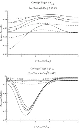
Figure 1: Coverage probability of several confidence intervals in the known-variance case, as a function of the scaled parameter ζ =
β2·M2/SD( ˆβ2·M2), using the model selection procedure with C = √
2, i.e., AIC. The nominal coverage probability is 1−α = 0.95, indicated by a gray horizontal line. The coverage target isβ1·Mˆ (top panel) and
β1·M2 (bottom panel). In each panel, the four solid curves are computed
forρ = 0.9, and the four dashed curves are forρ = 0.5. The curves in each group of four are ordered: Starting from the top, the curves show the coverage probabilities forKS(Scheff´e),KP (PoSI),KP1(PoSI1), and
KN (naive).
[image:11.612.180.433.120.531.2]resulting coverage probabilities depends on the correlation coefficient ρ, with larger values ofρcorresponding to smaller minimal coverage probabilities. But the strength of the effect varies greatly with the scenario, i.e., on whether the coverage target isβ1·Mˆ orβ1·M2. When the coverage target isβ1·Mˆ (top panel
in Figure 1), we see that the effect of model selection is comparatively minor: The smallest coverage probabilities are always obtained for the ‘naive’ interval, whose coverage probability here can be smaller as well as larger than the nominal 0.95. Irrespective of the true parameters, the actual coverage probability of the ‘naive’ interval is quite close to the nominal one here. The other intervals, i.e., the PoSI1-, the PoSI-, and the Scheff´e-interval, all have coverage probabilities larger than 0.95. [The minimal coverage probabilities here are obtained for
ζ= 0, but we found this not to be the case for other model selection procedures, i.e., for other values ofC.] When the coverage target isβ1·M2 (bottom panel in
Figure 1), however, we get a very different picture: Forρ = 0.9, the minimal coverage probability of all the intervals considered there is much smaller than 0.95, with minima between 0.55 (‘naive’) and 0.65 (Scheff´e). Forρ= 0.5, the minimal coverage probabilities of the ‘naive’ interval and of the PoSI1-interval are below, while those of the other intervals are above, the nominal 0.95. For very small values ofρ, the coverage probabilities of all the intervals considered in Figure 1 are visually indistinguishable from horizontal lines as a function ofζ
(and hence are not shown here), irrespective of the coverage target. Forρ= 0.1, for example, the coverage probability of the ‘naive’ interval is about 0.95, while that of the other intervals is above 0.95, ordered by their length. [This should not come as a surprise since in case ρ = 0 model selection has no effect on estimating the regression coefficients; furthermore, the two targets are identical in this case.]
Figure 1 illustrates that the coverage probability of confidence intervals post-model-selection depends crucially on whether the coverage target isβ1·Mˆ as in Berk et al. (2013) or the more classical coverage target β1·M2. We stress here
again that the PoSI-intervals and the Scheff´e-interval have not been designed to deal with the case where the coverage target isβ1·M2. For a more detailed
analysis of the ‘naive’ interval in the case where the coverage target isβ1·M2,
we refer to Kabaila and Leeb (2006).
For the other values ofCthat we consider, i.e., forC=plog(n) for various values ofn, we found the following: When the coverage target isβ1·Mˆ, the results are very similar to those shown in the top panel of Figure 1. To conserve space, we do not show these results here. When the target isβ1·M2, the resulting curves
are of the same shape but steeper, with coverage probabilities decreasing asC
increases. This is so because larger values ofClead to more frequent selection of the smaller modelM1, causing more bias in the resulting post-model-selection estimator; we refer to Leeb and P¨otscher (2005) and, in particular, Figure 3 in that reference, for further discussion and analysis of this phenomenon.
(PoSI), forKP1 (PoSI1), forKS (Scheff´e), and forK∗ (the smallest validK).
By construction, we haveK∗ ≤KP1≤KP ≤KS, so that the resulting curves
of minimal coverage probabilities are also arranged in increasing order.
��� ��� ��� ��� ��� ���
���� ���� ���� ���� ���� ����
ρ
��
��
�
��
����
��
��
�����
��
���
�
[image:13.612.181.431.174.341.2]������� �������� ����������� �� � �������� ��ρ
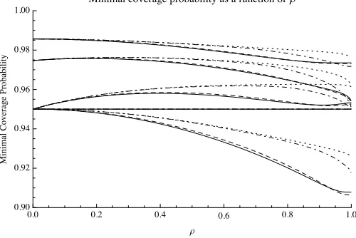
Figure 2: Minimal coverage probabilities of the confidence intervals for
β1·Mˆ as a function ofρ in the known-variance case, for C =
√
2 (solid curves), C = p
log(10) (dashed curves), C = p
log(100) (dot-dashed curves), and C = p
log(1000) (dotted curves). The nominal coverage probability is 1−α= 0.95. For each value ofC, the corresponding five curves are ordered: Starting from the top, the curves correspond to the intervals withKS,KP,KP1,K∗, andKN.
All the minimal coverage probabilities shown in Figure 2 are within 5% of the nominal level 0.95. For the ‘naive’ intervals corresponding toKN (the first
four curves from the bottom), the minimal coverage probability is below 0.95 (except for the trivial case where ρ = 0), but not by much. The intervals withK∗ have minimal coverage probabilities of exactly 0.95, for every value of
C, by construction (but note that K∗ depends on C whereas KS, KP, KP1, and KN do not). Hence, the curves corresponding to the K∗’s for the four
values of C considered here are constant and sit on top of each other. And, again by construction, all other intervals are slightly too large in the sense that their minimal coverage probability exceeds the nominal level 0.95. Concerning the influence ofC, we see that larger values of C correspond to slightly larger minimal coverage probabilities for the intervals corresponding toKN,KP1,KP,
andKS, and for most values ofρ; it should be noted, however, that – in contrast
to the case of the standard target – here the target changes with C. Overall, the difference between the coverage probabilities of all these intervals is not dramatic.
Lastly, we compare the confidence intervals for β1·Mˆ through the values of the constantsK that correspond to the intervals in question. By construction,
KS andKN are constant as a function ofρ. Note that the constantsKN,KP,
(and thus not onC), while the constantK∗does depend on the model selection
procedure (and thus onC). For a given model selection procedure, the constant
K∗ is the smallest numberK for which (2.2) holds; in particular, the interval
corresponding toKhas minimal coverage probability smaller/equal/larger than 1−αif and only ifK is smaller/equal/larger thanK∗.
��� ��� ��� ��� ��� ���
��� ��� ��� ��� ���
ρ
�
[image:14.612.181.432.198.366.2]��������� � �� � �������� ��ρ
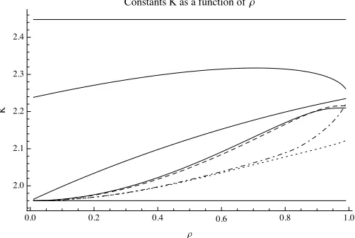
Figure 3: The constantsK that govern the width of the confidence in-tervals as a function of ρ in the known-variance case, using the model selection procedure with critical valueC. The nominal coverage probabil-ity is 1−α= 0.95. Starting from the top, the five solid curves showKS,
KP,KP1,K∗forC =
√
2 (AIC), and KN. The remaining curves show
K∗ forC =
p
log(10) (dashed curve), for C =p
log(100) (dash-dotted curve), and forC=p
log(1000) (dotted curve).
The interpretation of Figure 3 is similar to that of Figure 2, the main differ-ence being that the lengths considered here are somewhat more distorted than the minimal coverage probabilities considered earlier. The ‘naive’ interval is up to about 10% too short, while the intervals corresponding toKP1,KP, andKS
are too long, namely by up to about 5%, 15%, 25%, respectively. We also see thatK∗ decreases asC increases for most values ofρ, which is consistent with
the observations made in the second-to-last paragraph.
4
Simulation study
We now compare the ‘naive’ interval, the PoSI1 interval, and (a variant of) the PoSI interval for β1·Mˆ by their respective minimal coverage probabilities in a simulation study where the data are generated from a Gaussian overall linear modelMfull, say, of the formY =Xβ+uwith 30 observations, 10 explanatory variables, and i.i.d. standard normal errors. Moreover, we also study these intervals when the coverage target isβ1 = β1·Mfull (instead of β1·Mˆ). For the
the overall model; hence, we haver=n−p= 20 here. [To be precise, while the constantsKN as well asKP1are computed as detailed in Section 2, we consider instead ofKP defined by (2.3) the larger constant KP′ which is obtained from
(2.3) whenMis replaced by the collection ofallnon-empty subsets of{1, . . . , p}. We shall refer to the resulting interval also as a PoSI-interval in this section. The reason for this choice is that code for computingKP′ is publicly available
from the authors of Berk et al. (2013), so thatKP′ is the PoSI-constant likely
to be used by practitioners. Note thatKP1≤KP ≤KP′ holds, and hence the
performance of the interval based onKP can be easily deduced from Table 1.]
As model selectors, we consider AIC, BIC, and the LASSO: For AIC we use
thestep()function in R with its default settings, subject to the constraint that
the regressor of interest, i.e., the first one, is always included; this corresponds to minimizing the AIC objective function through a greedy general-to-specific search over the 29 candidate models (i.e.,
M consists of all submodels of the overall model that contain the first regressor). Similarly, for BIC we use the
step() function with the penalty parameter equal to log(30). And for the
LASSO, we basically select those regressors for which the LASSO-estimator has non-zero coefficients. [More precisely, we use thelars package in R and follow suggestions outlined in Efron et al. (2004, Sect.3.4): To protect the regressor of interest (the first one), we first compute the residual of the orthogonal pro-jection ofy on the first regressor; write ˜y for this residual vector, and write ˜X
for the regressor matrixX with the first column removed. We then compute the LASSO-estimator for a regression of ˜y on ˜X using the lars() function; the LASSO-penalty is chosen by 10-fold cross-validation using the cv.lars() function (in both functions, we set the intercept parameter to FALSE, and otherwise use the default settings). The selected model is comprised of those regressors in ˜X for which the corresponding LASSO coefficients are non-zero, plus the first column ofX.]
Three designs are considered for the design matrixX: For design 1, we take the regressor matrix from the data-example from Section 3 of Kabaila and Leeb (2006) (for which the minimal coverage probability of a ‘naive’ nominal 95% interval forβ1, based on a different variance estimator, was found to be no more than 0.63 in that paper). For design 2 and 3, respectively, we consider the exchangeable design and the equicorrelated design studied in Sections 6.1 and 6.2 of Berk et al. (2013). The exchangeable design is such that the corresponding PoSI-constant is small asymptotically, and the equicorrelated design corresponds to a large PoSI-constant asymptotically; cf. Theorem 6.1 and Theorem 6.2 in Berk et al. (2013). For the equicorrelated design (design 3), the difference between the PoSI-interval and the ‘naive’ interval is thus expected to be most pronounced.
surface absorbency index (0 = complete absorbency; 100 = no absorbency), estimated soil storage capacity (inches of water), infiltration rate of water into soil (inches/hour), time period during which rainfall exceeded 1/4 inch/hour, and a constant term to include an intercept in the model. Logarithms are taken of the response and of all explanatory variables except for the intercept. For the second design, we defineX(p)(a) as in Section 6.1 in Berk et al. (2013) with
p= 10 and we choose a = 10 here, and we set X =UX(p)(a), where U is a collection ofporthonormaln-vectors obtained by first drawing a set ofpi.i.d. standard Gaussiann-vectors and then applying the Gram-Schmidt procedure. And for the third design, we define X(p)(c) as in Section 6.2 in Berk et al. (2013), but such that the regressor of interest is the first one, where we choose
c=p
0.8/(p−1), and we setX =VX(p)(c), whereV is obtained by drawing an independent observation from the same distribution as U before. [Because we consider only orthogonally invariant methods here, the coverage probabilities under study are invariant under orthogonal transformations of the columns of the design matrix. In particular, the coverage probabilities for the second and for the third design actually do not depend on the matricesU andV.]
For each of the three design matrices, we simulate coverage probabilities un-der the model Y = Xβ+u for randomly selected values of the parameter β, we identify those β’s for which the simulated coverage probability gets small, and we correct for bias as explained in detail shortly. For example, consider the case where the coverage target isβ1 and where the ‘naive’ confidence inter-val is used with AIC as the model selector. We first select 10,000 parameters
β by drawing i.i.d. samples from a random p-vector b such that Xb follows a standard Gaussian distribution within the column-space of X. For each of these β’s, we approximate the corresponding coverage probability by the cov-erage rate obtained from 100 Monte Carlo samples. In particular, we draw 100 Monte Carlo samples from the overall model usingβ as the true parameter. For each Monte Carlo sample, we compute the model selector ˆM and the resulting ‘naive’ confidence interval, and we record whetherβ1is covered or not. The 100 recorded results are then averaged, resulting in a coverage rate that provides an estimator for the coverage probability of the interval if the true parameter isβ. After repeating this for each of the 10,000 β’s, we compute the resulting smallest coverage rate as an estimator for the minimal coverage probability of the confidence interval. The smallest coverage rate, as an estimator for the smallest coverage probability, is clearly biased downward. To correct for that, we then take those 1,000 parameters β that gave the smallest coverage rates and re-estimate the corresponding coverage probabilities as explained earlier, but now using 1,000 Monte Carlo samples. For that parameter β that gives the smallest coverage rate in this second run, we run the simulation again but now with 500,000 Monte Carlo samples, to get a reliable estimate of the corre-sponding coverage probability. This procedure is also used, mutatis mutandis, to evaluate the performance of the PoSI1-interval and of the PoSI-interval (with constantKP′), with AIC, BIC and the LASSO as model selectors, and also in
by a stochastic search over a 10-dimensional parameter space, and thus only provide approximate upper bounds for the true minimal coverage probabilities (cf., for example, the results for the PoSI-interval and the PoSI1-interval, when the coverage target isβ1, when BIC is used for model selection, and when the second design matrix is used forX). Table 1 summarizes the results.
Coverage Model Confidence Design 1 Design 2 Design 3 Target Selector Interval (watershed) (exchangeable) (equicorr.)
β1·Mˆ
AIC
PoSI 1.00 1.00 0.99
PoSI1 0.99 0.99 0.98
Naive 0.89 0.92 0.81
BIC
PoSI 1.00 1.00 0.99
PoSI1 0.98 0.99 0.98
Naive 0.89 0.86 0.84
LASSO
PoSI 1.00 1.00 1.00
PoSI1 1.00 1.00 1.00
Naive 0.95 0.95 0.93
β1
AIC
PoSI 0.85 0.91 0.83
PoSI1 0.76 0.91 0.77
Naive 0.62 0.82 0.54
BIC
PoSI 0.62 0.65 0.48
PoSI1 0.51 0.66 0.43
Naive 0.43 0.51 0.26
LASSO
PoSI 0.09 0.12 0.05
PoSI1 0.08 0.12 0.03
[image:17.612.135.491.203.450.2]Naive 0.07 0.10 0.01
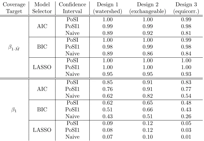
Table 1: Smallest coverage probabilities (rounded to two digits of ac-curacy after the comma) found in MC study for the coverage targets
β1·Mˆ, andβ1, using AIC, BIC, and the LASSO for model selection, for the PoSI-interval, the PoSI1-interval, and the ‘naive’ interval, each with nominal coverage probability 0.95.
close to, or below, 0.5 in some cases. This is because BIC selects smaller mod-els than AIC, typically causing more bias in the resulting post-model-selection estimator (that phenomenon is analyzed in greater detail in Leeb and P¨otscher (2005) and P¨otscher (2009)). The results for the LASSO stand out: When the coverage target isβ1·Mˆ, the PoSI1-interval (resp. PoSI-interval) gives smallest probabilities very close to one, while the smallest coverage probability of the naive interval is very close to the nominal level (0.95). But when the coverage target isβ1, all intervals have smallest coverage probabilities of around 0.1 and below. The reason for this is that the LASSO model selector, as implemented here and for the parameters used in the stochastic search for the smallest cov-erage probability, selects the smallest possible model in most cases, i.e., the model containing only the first regressor. In other words, the model selected by the LASSO is ‘nearly non-random.’ When the target is β1·Mˆ, this entails that the naive interval is approximately valid and that both PoSI intervals are too large. [Indeed, the naive interval is valid if the underlying model selector always chooses a fixed (non-random) model; cf. the discussion following (2.2).] But when the target is β1, the model selected by the LASSO typically suffers from severe bias, resulting in very small coverage probabilities for all intervals. Other model selectors can, of course, give results different from those in Ta-ble 1. The model selectors chosen here represent a selection of popular methods from the contemporary literature that exhibit an interesting range of possible scenarios for the minimal coverage probabilities of confidence intervals post-model-selection.
Acknowledgments
We thank the anonymous referee and the editor for helpful comments and feed-back. We also thank Richard Berk, Lawrence Brown, Andreas Buja, Kai Zhang, and Linda Zhao for providing us with the code to compute the PoSI-constant
KP′ used in Section 4; the entire “PoSI-group” at the University of
Pennsyl-vania for inspiring discussions during Hannes Leeb’s visit; and Francois Bachoc for constructive feedback. Karl Ewald gratefully acknowledges financial sup-port from Deutsche Forschungsgemeinschaft (DFG) grant FOR916, and Hannes Leeb’s research is partially supported by FWF grant P26354.
Appendix:
Confidence
sets
under
zero-restrictions post-model-selection
Letyand ˆσ2
be as in Section 2, and considerM={M0, M1}, where each of the two
candidate modelsMiis full-rank. Suppose we are interested in the coefficient of the
first regressorX1, that is assumed present inM1 but absent inM0. In the notation
introduced in Section 2, we thus have 1 ∈ M1 and 1 6∈ M0. Let ˆM be any model
selection procedure that chooses only betweenM0 and M1. As the model-dependent
coverage target, we consider the coefficient ofX1, which is not restricted underM1, and
and let the target be bMˆ. We consider a ‘naive’ confidence interval for bMˆ that is
defined as
IMˆ =
ˆ
β1·M1±kNσˆ1·M1 if ˆM=M1
{0} if ˆM=M0,
wherekN is chosen so thatPµ,σ(β1·M1 ∈βˆ1·M1±kNσˆ1·M1) = 1−α. [The constantkN
is the (1−α/2)-quantile of a standard normal distribution in the known-variance case and the (1−α/2)-quantile of at-distribution withrdegrees of freedom in the unknown-variance case.] The actual coverage probability ofIMˆ, as a confidence interval forbMˆ,
is at least equal to the nominal coverage probability 1−α, because
Pµ,σ(bMˆ ∈IMˆ)
= Pµ,σ(β1·M1∈IM1 and ˆM =M1) + Pµ,σ(0∈ {0},Mˆ =M0)
= Pµ,σ(β1·M1∈IM1 and ˆM =M1) + Pµ,σ( ˆM 6=M1)
= Pµ,σ(β1·M1∈IM1 or ˆM 6=M1) ≥ 1−α,
where the inequality in the last step holds in view of the choice ofkN.
References
D. W. K. Andrews and P. Guggenberger. Hybrid and size-corrected subsampling methods. Econometrica,77:721–762, 2009.
R. Berk, L. Brown, A. Buja, K. Zhang, and L. Zhao. Valid post-selection inference.
Ann. Statist.,41:802–837, 2013.
P. J. Bickel and K. A. Doksum. Mathematical Statistics: Basic Ideas and Selected
Topics. Holden-Day, Oakland, 1977.
L. D. Brown. The conditional level of Student’s t test.Ann. Math. Stat.,38:1068–1071, 1967.
R. J. Buehler and A. P. Feddersen. Note on a conditional property of Student’s t.
Ann. Math. Stat.,34:1098–1100, 1963.
P. Craven and G. Wahba. Smoothing noisy data with spline functions. Estimating the correct degree of smoothing by the method of generalized cross-validation. Numer. Math.,31:377–403, 1978.
T. K. Dijkstra and J. H. Veldkamp. Data-driven selection of regressors and the boot-strap.Lecture Notes in Econom. and Math. Systems,307:17–38, 1988.
B. Efron, T. Hastie, I. Johnstone, and R. Tibshirani. Least angle regression. Ann. Statist.,32:407–499, 2004.
K. Ewald. On the influence of model selection on confidence regions for marginal associations in the linear model. Master’s thesis, University of Vienna, 2012. P. Kabaila. Valid confidence intervals in regression after variable selection.
P. Kabaila. The coverage properties of confidence regions after model selection. Int. Statist. Rev.,77:405–414, 2009.
P. Kabaila and H. Leeb. On the large-sample minimal coverage probability of confi-dence intervals after model selection. J. Amer. Statist. Assoc.,101:619–629, 2006. H. Leeb. The distribution of a linear predictor after model selection: unconditional
finite-sample distributions and asymptotic approximations. IMS Lecture Notes -Monograph Series,49:291–311, 2006.
H. Leeb. Evaluation and selection of models for out-of-sample prediction when the sam-ple size is small relative to the comsam-plexity of the data-generating process.Bernoulli,
14:661–690, 2008.
H. Leeb and B. M. P¨otscher. The finite-sample distribution of post-model-selection estimators, and uniform versus non-uniform approximations. Econometric Theory,
19:100–142, 2003.
H. Leeb and B. M. P¨otscher. Model selection and inference: Facts and fiction. Econo-metric Theory,21:21–59, 2005.
H. Leeb and B. M. P¨otscher. Can one estimate the conditional distribution of post-model-selection estimators? Ann. Statist.,34:2554–2591, 2006a.
H. Leeb and B. M. P¨otscher. Performance limits for estimators of the risk or dis-tribution of shrinkage-type estimators, and some general lower risk-bound results.
Econometric Theory,22:69–97, 2006b.
H. Leeb and B. M. P¨otscher. Can one estimate the unconditional distribution of post-model-selection estimators? Econometric Theory,24:338–376, 2008a. H. Leeb and B. M. P¨otscher. Model selection. In T. G. Andersen, R. A. Davis, J.-P.
Kreiß, and Th. Mikosch, editors,Handbook of Financial Time Series, pages 785–821, New York, NY, 2008b. Springer.
R. A. Olshen. The conditional level of the F-test.J. Amer. Statist. Assoc.,68:692–698,
1973.
B. M. P¨otscher. Effects of model selection on inference. Econometric Theory, 7: 163–185, 1991.
B. M. P¨otscher. The distribution of model averaging estimators and an impossibility result regarding its estimation.IMS Lecture Notes - Monograph Series,52:113–129,
2006.
B. M. P¨otscher. Confidence sets based on sparse estimators are necessarily large.
Sankhya,71:1–18, 2009.
B. M. P¨otscher and H. Leeb. On the distribution of penalized maximum likelihood estimators: The LASSO, SCAD, and thresholding. J. Multivariate Anal., 100:
2065–2082, 2009.
B. M. P¨otscher and U. Schneider. Confidence sets based on penalized maximum likelihood estimators in Gaussian regression. Electron. J. Statist.,4:334–360, 2010. B. M. P¨otscher and U. Schneider. Distributional results for thresholding estimators in high-dimensional Gaussian regression models. Electron. J. Statist.,5:1876–1934, 2011.
J.O. Rawlings. Applied Regression Analysis: A Research Tool. Springer Verlag, New York, NY, 1998.
P. K. Sen. Asymptotic properties of maximum likelihood estimators based on condi-tional specification. Ann. Statist.,7:1019–1033, 1979.
P. K. Sen and E. A. K. Md. Saleh. On preliminary test and shrinkage M-estimation in linear models. Ann. Statist.,15:1580–1592, 1987.