A Theorem on the Limit Properties of Structural Change and some Implications

A Theorem on the Limit-Properties of

Structural Change and some Implications

Stijepic, Denis

Fernuniversität in Hagen (University of Hagen)

25 June 2014

Online at

https://mpra.ub.uni-muenchen.de/57580/

A theorem on the limit-properties of structural change and

some implications

Stijepic, Denis*

University of Hagen

June 2014

Abstract

Recent growth literature studies structural change in relatively specific three-sector growth models with a focus on the agriculture-manufacturing-services structure. In this paper we take another approach for studying this structural change. By using only few axioms on the properties of structural change trajectories and some mathematical theorems on the limit-properties of trajectories in the plane, we show that structural change in a three-sector framework is a relatively simple process: it is either transitory or cyclical unless there are some “exogenous” driving forces. We elaborate the implications of this result for the structural change modelling literature and topics for further research.

JEL-Codes: C61, O41

Keywords: structure, dynamics, differential equation systems, limit, Poincaré-Bendixon-theory.

*Address: Fernuniversitaet in Hagen, Fachbereich Wirtschaftswissenschaften, Universitaets-strasse 41, D-58084 Hagen, Germany. Phone: +49(0)2331/987-2640.

E-mail: [email protected].

1. INTRODUCTION

Recent growth literature studies structural change in relatively specific micro-founded

growth models with a focus on the three-sector structure

(agriculture-manufacturing-services).1 In this paper we take another approach for studying this structural change.

By using only few axioms on the properties of structural change trajectories and some

mathematical theorems on the limit-properties of trajectories in the plane (among

others Poincaré-Bendixon theory), we show that structural change in a three-sector

framework is a relatively simple process: it is either transitory or cyclical unless there

are some “exogenous” forces (e.g. technological progress or capital accumulation)

which drive it. We derive the implications of this result for the structural change

modelling literature and elaborate topics for further research.

In the next section we derive the properties of structural change. Section 3 discusses

the implications of our results.

2. A THEOREM ON THE PROPERTIES OF STRUCTURAL CHANGE

The structural change literature studies the dynamics of sectoral employment-shares

and/or sectoral GDP-shares. The employment-share of sector i is given by L_i /L,

where L_i is the number of employees in sector i and L is the number of employees in

the whole economy. Analogously, the GDP-share of sector i is given by GDP_i/GDP,

where GDP_i is the value added by sector i and GDP is the value added by all sectors.

Definition 1: Let s_i(t) denote the employment-share of sector i (or the GDP-share of

sector i), i=1,2,3. The structure of the economy at time t is given by the vector

3 3

2

1( ), ( ), ( )) (

: )

(t = s t s t s t ∈ℜ

s , which satisfies the following conditions:

(1) si(t)≥0 ∀t i=1,2,3

(2) s1(t)+s2(t)+s3(t)=1 ∀t

1

It is obvious that, since si(t) stands for the employment- or GDP-share of sector i, (1)

and (2) are satisfied: employment and output cannot be negative; furthermore, the

sum of “shares” must be equal to one.

Definition 2: Structural change refers to a continuous change in s(t) over some

finite or infinite period of time.

Thus, in this paper we do not analyse abrupt changes (jumps) in the structure of the

economy. Structural change is a continuous process, like in the previous literature.

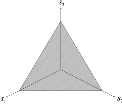
Definition 3: The domain of structural change (∆) is the set of all points s(t)

satisfying Def. 1: ∆:={s(t)∈ℜ3:s_i(t)≥0 for i=1,2,3; s₁(t)+s₂(t)+s₃(t)=1}.

Lemma 1: ∆ is a compact convex subset of the plane. (Cf. Figure 1.)

Proof: The definition of ∆ implies that ∆ is a standard 2-simplex; cf. e.g. Border (1985), p.20. It is well-known that the 2-simplex is a compact convex subset of the

plane; cf. e.g. Munkres (1984), p.2f. On 2-simplexes and structural change see

Stijepic (2014a). 

In the previous literature structural change is modelled by using (vector) differential

equations or continuous flows. These equations and flows are derived from economic

theories, e.g. optimization problems of rational individuals (producers, households,

etc.). In the following we do not require such a micro-foundation; we study the

typical differential equation (cf. Assumption 1) and/or the typical continuous flow (cf.

Assumption 2) describing structural change.

Assumption 1: The dynamics of s(t) are given by the following differential equation:

(3) s_(t)=Φ₍s_(t),x(_t)_), s_(t)∈S ⊆∆_,t∈ℜ

(4) = ∈S

where:Φ(.) is a vector-function; S _{is a connected subset of} ∆_{; s0 is given;} x_{(t) is}

a vector of real-valued “exogenous” variables.

Several aspects of this assumption are noteworthy: a) The system (3)-(4) is very general; it covers most, if not all, of the previous literature (on continuous-time

structural change modelling). b) In general, economic theories may generate differential equations which are not defined on whole ∆. Thus, we assume that the

differential equation (3) is defined on a subset S _of ∆_{. (Cf. Figure 2.)} c) _{In general,} the initial value s₀ is given by observable data; see some of the previous literature for

examples. d) In general, the structural dynamics are not only determined by the structural variables s(t) but also by some other variables x(t) which we name “exogenous” variables. The latter variables are “exogenous” in the sense that (in part)

they are explained outside the structural system (3). In the previous literature such

“exogenous” variables are, e.g., technological progress or capital.

Assumption 2: If x(t)=x=const.∀t, there exists a unique continuous solution φ(t)

of the initial value problem (3)-(4) passing through s₀ at t=0. The structure of the

economy associated with this solution is given by s(t)=φ(t)∈S _, ∈ℜ ₊

0

t .

Assumption 2 refers to a continuous solution due to Definition 2. Furthermore, the

existence of a unique continuous solution (Assumption 2) is a standard assumption in

economic and mathematical literature; see Stijepic (2014b) for examples of economic

literature; on mathematical aspects see any (introductory) book on differential

equations, e.g. Hale (2009), p.18f and p.38.

Definition 4: τ is the (positive) (semi-)trajectory associated with the solution φ(t),

A solution (φ(t)) of the initial value problem (3)-(4) can be represented by a

trajectory (τ); cf. Definition 4. In our paper this trajectory is a continuous curve in

S _{. (Cf. Figure 3.)}

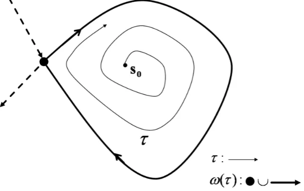
Definition 5: Structural change is transitory if s(t) is constant in the limit, i.e. if

* s s = ∞ → ( )

lim t

t

S

∈ .

Thus, transitory structural change means that the structure converges to a steady state

*

s , i.e. a state where the structure does not change. (Cf. Figure 3.)

Definition 6: Structural change is cyclical on the interval (t₁,t₂), if there exist a real

number a>0 such that s(t)=s(t−a) for t₁ <t<t₂.

Hence, cyclical structural change means that the economy repeats one and the same

structural change pattern (cycle) again and again. In this case the trajectory (τ) is a

closed curve (or: Jordan curve), e.g. a circle, contained in S _{; the economy moves}

along this curve and completes the cycle (infinitely) many times. (Cf. Figure 3.)

Theorem 1: If Assumptions 1 and 2 are satisfied and if there are no exogenous

structural change drivers (i.e. if x(t)=x=const.∀t), structural change is transitory or cyclical for all t or cyclical in the limit.

Proof: The assumptions in our paper imply that the differential equation system analysed here has the following properties:

(a) It is autonomous; cf. (3) and x(t)=x=const.∀t.

(b) It is defined on a bounded subset (S _{) of the plane; cf. Assumption 1 and Lemma}

1. Thus, τ (cf. Definition 4) is a bounded trajectory in the plane.

(c) It generates continuous and unique solutions; cf. Assumption 2.

It is well known that under these conditions the following lemma is true.

Lemma 2: Let ω(τ) denote the positive limit set of τ. If conditions (a)-(c) are

(i) ω(τ) is a fixed point (“critical point”).

(ii) ω(τ) is a closed curve (“cycle”).

(iii) ω(τ) is a homoclinic orbit (including its fixed point).

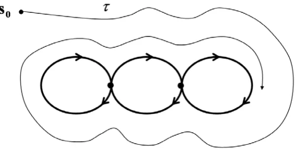
(iv) ω(τ) is a union of at least two fixed points and the trajectories

connecting them (“heteroclinic union”).

Note that the term “heteroclinic union” is not common in the literature; we use it here

as an abbreviation. Furthermore, note that a “heteroclinic union” must contain

heteroclinic trajectories and can contain homoclinic trajectories. For detailed proof

and extensive discussion of Lemma 2 see e.g. Andronow et al. (1965), Chapter VI§2,

in particular p.386f (section 4), Guckenheimer and Holmes (1990), p.45, Hale (2009),

p.55 (Theorem 1.5), or Teschl (2011), Chapter 7.3.

Lemma 2 implies almost directly Theorem 1, as we will see now.

In case (i) (cf. Lemma 2) the economy converges along trajectory τ(cf. Definition 4)

to a fixed point s*, i.e. ω(τ)=s*. That is, the solution φ(t) (cf. Assumption 2) converges to a fixed point s* for t→∞. Thus, structural change is transitory; cf. Definition 5.

Case (ii) (cf. Lemma 2) is known from the Poincaré-Bendixon theory; see e.g. Miller

and Michel (2007), p.290ff, or Hale (2009), p.51ff. ω(τ) is a closed curve. Thus, τ

is either a non-closed trajectory converging to a closed curve (i.e. the economy

converges to a “limit cycle”) or a closed trajectory (“Jordan curve”). Thus, structural

change is cyclical in the limit or cyclical for all t; cf. Definition 6.

In cases (iii) and (iv) (cf. Lemma 2) the solution φ(t) converges for t→∞ to (all)

the points of the homoclinic orbit or to (all) the points of the “heteroclinic union”, per

definition of the term “positive limit set” (ω(τ)). Therefore, structural change is

cyclical in the limit; cf. Definition 6. (Cf. Figures 4 and 5.) 

3. IMPLICATIONS

Theorem 1 shows that three-dimensional structural change is a relatively simple

behaviour. This result has interesting implications for the existing structural change

modelling literature and for further research:

1.) The number of sectors is an important modelling decision. The simple behaviour

expressed in Theorem 1 is a property of three-sector models. In higher-dimensional

models the dynamics can be more complicated. The theoretical implications of the

sensitivity of model predictions to the choice of number of sectors should be

elaborated.

2.) The previous literature (cf. Footnote 1) predicts that structural change is transitory.

That is, it predicts that the economic structure in today’s very advanced economies,

which is characterised by prevalence of services, will not change significantly in the

future. In contrast, if we allow for cyclical structural change (cf. Theorem 1), we may

expect significant structural change in the future (e.g. a return to a “prevalence of

manufacturing”).

3.) The previous literature (cf. Footnote 1) models structural change in a simplistic

way: in this literature structural change is driven by “exogenous drivers” x(t) and, in particular, by capital accumulation and technological progress. That is, when using

our notation, the following statement is true for the previous literature: if

t const

t)= .∀

(

x , then s(t)=const.∀t. (For two examples see the optional APPENDIX.) In contrast, our Theorem 1 implies that, even if x(t)=const.∀t, transitory structural change can exist. This transitory structural change may be an

important component of real-life structural change, since transitory processes can

explain a lot of dynamics if their convergence-speed is low. Therefore, it seems to be

interesting to elaborate the empirical implications and theoretical foundations of this

transitory structural change component.

LITERATURE

Acemoglu, D., Guerrieri, V. (2008). Capital Deepening and Non-Balanced Economic Growth. Journal of Political Economy, 116(3):467-498.

Verlag, Berlin. English translation (Andronov, A.A., Vitt, E.A., Khaiken, S.E. [1966]

“Theory of Oscillators”) is published by Pergamon Press, Oxford.

Border, K.C. (1985). Fixed Point Theorems with Applications to Economics and Game Theory. Cambridge University Press, Cambridge.

Buera, F.J., Kaboski, J.P. (2009). Can Traditional Theories of Structural Change Fit the Data? Journal of the European Economic Association, 7(2-3):469-477.

Foellmi, R., Zweimuller, J. (2008). Structural change, Engel's consumption cycles and Kaldor's Facts of Economic Growth. Journal of Monetary Economics,

55(7):1317-1328.

Guckenheimer, J., Holmes, P. (1990). Nonlinear Oscillations, Dynamical Systems, and Bifurications of Vector Fields. Springer, New York.

Hale, J.H. (2009). Ordinary Differential Equations. Dover Publications, Mineola, New York.

Herrendorf, B., Rogerson, R., Valentinyi, Á. (2014). Growth and Structural Transformation. In: Aghion P. and S.N. Durlauf, eds., “Handbook of Economic

Growth”, Volume 2B, Elsevier B.V.

Kongsamut, P., Rebelo, S., Xie, D. (2001). Beyond Balanced Growth. Review of Economic Studies, 68(4):869-882.

Kruger, J.J. (2008). Productivity and Structural Change: A Review of the Literature. Journal of Economic Surveys, 22(2):330–363.

Miller, R.K., Michel, A.N. (2007). Ordinary Differential Equations. Dover Publications, Mineola, New York.

Munkres, J.R. (1984). Elements of Algebraic Topology. Addison-Wesley, Menlo Park, California.

Ngai, R.L., Pissarides, C.A. (2007). Structural Change in a Multisector Model of Growth. American Economic Review, 97(1):429-443.

Stijepic, D. (2014a). A Geometrical Approach to Structural Change Modeling. Available at: http://ideas.repec.org/p/pra/mprapa/55010.html

Stijepic, D. (2014b). Structural Change in Neoclassical Growth Literature. Available

at: http://papers.ssrn.com/sol3/cf_dev/AbsByAuth.cfm?per_id=1636491

OPTIONAL FIGURES

Figure 1: ∆ (shaded area) in the Cartesian coordinate system.

Figure 3: Examples: transitory and cyclical structural change.

Figure 5: Example: ω(τ) is a “heteroclinic union”.

structural change is only driven by „exogenous” drivers, i.e. the endogenous transitory

component emphasized by Theorem 1 is neglected in the previous literature. This is not a

critique of the previous literature; the previous literature has correctly derived its statements

from the neoclassical modelling framework. Rather, the following discussion should show

which types of structural change are not studied in the previous literature; the knowledge of

these neglected types is important for further research (new approaches to modelling).

Kongsamut et al. (2001) show on p.877 that sectoral employment-shares are given by the

following equations in their model:

(A.1) ) 1 , (k F X B A g N t A A

t =−

 _, M ₌₀

t

N ,

) 1 , (k F X B S g N t S S t = 

where: N_tA, N_tM and N_tS are the employment-shares of agriculture, manufacturing and

services, respectively, at time t; A,S,B_A,B_S and X_t are exogenous parameters; F(.) is the

production function; k is capital in efficiency units; g is the growth rate of exogenous

technological progress. We can see immediately that, if there are no exogenous structural

change drivers (g=0), structural change does not take place. In contrast, our Theorem 1 shows

that, even if there are no exogenous structural change drivers, (transitory or cyclical)

structural change can arise.

In the Ngai/Pissarides (2007)-model employment-shares are given by the following equation

(see there equation (13)):

(A2) y c X x n i i = i

n is the employment-share of sector i. x_i/X is a function of exogenous parameters. c and y

are variables which are independent of n_i; cf. Ngai and Pissarides (2007), equations (24), (25)

and (12). Thus, if we use the terminology introduced in our paper, x_i/X , c and y are

“exogenous variables”. Then, we can express (A2) as follows when using our notation:

(A3) s(t)=Φ(x(t))

where x(t) is the vector of all “exogenous variables”, as defined in Assumption 1.

This equation shows the key difference between our model and the Ngai/Pissarides-model.