ISSN Online: 2327-5227 ISSN Print: 2327-5219
DOI: 10.4236/jcc.2017.56005 April 28, 2017
Performance Prediction Based on Statistics of
Sparse Matrix-Vector Multiplication on GPUs
*
Ruixing Wang
1, Tongxiang Gu
2#, Ming Li
31Country Graduate School of Chinese Academy of Engineering Physics, Beijing, China
2Laboratory of Computational Physics, Institute of Applied Physics and Computational Mathematics, Beijing, China 3Country Xi’an Aeronautics Computing Technique Research Institute, AVIC, Xi’an, China
Abstract
As one of the most essential and important operations in linear algebra, the performance prediction of sparse matrix-vector multiplication (SpMV) on GPUs has got more and more attention in recent years. In 2012, Guo and Wang put forward a new idea to predict the performance of SpMV on GPUs. However, they didn’t consider the matrix structure completely, so the execu-tion time predicted by their model tends to be inaccurate for general sparse matrix. To address this problem, we proposed two new similar models, which take into account the structure of the matrices and make the performance prediction model more accurate. In addition, we predict the execution time of SpMV for CSR-V, CSR-S, ELL and JAD sparse matrix storage formats by the new models on the CUDA platform. Our experimental results show that the accuracy of prediction by our models is 1.69 times better than Guo and Wang’s model on average for most general matrices.
Keywords
Sparse Matrix-Vector Multiplication, Performance Prediction, GPU, Normal Distribution, Uniform Distribution
1. Introduction
Sparse matrix-vector multiplication (SpMV) is an essential operation in solving linear systems and eigenvalue problems. For many iterative methods, the frac-tion of the execufrac-tion time of SpMV may be more than 80% in the total time, so the study of its performance has attracted a lot of attention. Right now, the GPU has been from a graphics accelerator to a computing device with a broad spec-trum of purposes, due to the characteristics of the multi-thread, high memory *The project is partly supported by the NSF of China (61472462, 11671049) and foundation of Key Laboratory of Computational Physics.
How to cite this paper: Wang, R.X., Gu, T.X. and Li, M. (2017) Performance Predic-tion Based on Statistics of Sparse Ma-trix-Vector Multiplication on GPUs. Jour-nal of Computer and Communications, 5, 65-83.
https://doi.org/10.4236/jcc.2017.56005
Received: March 17, 2017 Accepted: April 25, 2017 Published: April 28, 2017
Copyright © 2017 by authors and Scientific Research Publishing Inc. This work is licensed under the Creative Commons Attribution International License (CC BY 4.0).
http://creativecommons.org/licenses/by/4.0/
bandwidth. It can solve massively parallel problems and obtain very high per-formance. However, how to predict the execution time of SpMV on GPUs accu-rately is still a big challenge.
In 2003, Bolz et al. [1] first implemented conjugate gradient (CG) method on GPU which contains SpMV. Bell and Garland [2] proposed SpMV CUDA ker-nels for some well-known sparse matrix storage formats, such as compressed sparse row (CSR), Ellpack-Itpack (ELL), Coordinate (COO), Diagonal (DIA) and Hybrid (HYB). The jagged diagonal format (JAD) was used to implement the SpMV kernel in [3], and they also realized the GPU-accelerated precondi-tioned CG and GMRES methods. In this paper, we utilize the SpMV kernels in [3]: CSR-V, CSR-S, ELL and JAD.
In order to improve the performance of SpMV on GPUs, Vazquez et al. [4] presented a new sparse storage format, termed ELLR-T, which is improved from ELL format, to achieve higher performance. Monakov et al. [5] put forward a sliced ELL format and used auto-tuning to find the optimal configuration for batter performance. Zheng and Gu [6] proposed bisection ELL (BiELL) and bi-section JAD (BiJAD) format based on ELL and JAD format for optimizing SpMV on GPUs. Especially for irregular matrices, BiELL and BiJAD format can get greater load balance and higher performance by adjusting the elements sto-rage location of matrix and make the zero-padding less. Meanwhile, they rea-lized CG and GMRES method with BiELL and BiJAD format on GPU [7]. Choi et al. [8] designed blocked ELL format and select proper parameters for better performance. Guo et al. [9] proposed an auto-tuning framework that can select the parameters of SpMV kernels to obtain the optimal performance on GPUs.
ma-trices will be generated according to a GPU’s architecture features and four dif-ferent sparse matrix storage formats, then SpMV with these benchmark matrices are implemented on the GPU to obtain the execution times. We will establish two parametric models according to the results of the benchmark matrices and predict the execution time of the SpMV kernels with a given target matrix on the GPU by our models in second phase.
The performance prediction models are essentially at the statistical point of view to predict the execution time of different SpMV kernels on GPUs. Firstly, the execution time of the benchmark matrices with different parameters is re-quired, and then fitting the prediction functions according to the execution time of the benchmark matrices and two parameters. Finally, the estimated execution time of a target matrix will be got after putting two parameters into the predic-tion funcpredic-tions.
Compared with [16]’s model, the important difference of this paper is gene-rating benchmark matrices. In [16], the number of non-zero elements per row (PNZ) of the benchmark matrices is set to a fixed value. While in many practical
problems, such as in computer science or mathematics, there are many matrices are in irregular structure, which PNZ is different largely. So if PNZ of
bench-mark matrices generated is fixed, the performance prediction model will go awry to some extent and then the accuracy of prediction will be decreased. Keeping this in mind that we generated two kinds benchmark matrices whose PNZ in
the uniform distribution or normal distribution, respectively, and then establish its own performance prediction model. In the numerical experiments, we used our model to estimate the execution time of different SpMV kernels with 30 ma-trices, these matrices are from the University of Florida Sparse matrix collection [17]. The experimental results show that the average prediction error of our models are two to three times lower than [16] at least, some matrix even tens of times lower.
The remainder of this paper is organized as follows: Section 2 gives some pre-liminaries and Section 3 shows the details of the performance prediction model. Experimental results and analyses are reported in Section 4. Finally, some con-clusions and future works are stated in Section 5.
2. Preliminaries
ar-chitecture [14]. In addition, when a multiprocessor is given one or more thread blocks to execute, it partitions them into groups of 32 parallel threads termed warp.
Four sparse matrix storage formats used in our model are described below. The CSR is probably the most popular format for storing general sparse matrices [19]. To parallelize the SpMV for a matrix in the CSR format, a simple scheme called CSR-S (CSR scalar) kernel [2] is to assign each thread by one row. The main drawback of this scheme is that the pattern of memory access is un-coalesced, so it shows not very efficient. A better approach, termed CSR-V (CSR vector) is proposed in [2] and modified in [3] to realize the memory access contiguously. [2] assign a warp (32 threads) to each row, while [3] assign each row a half-warp (16 threads). In this approach, since all threads within a warp or a half-warp access non-zero elements of one row, these accesses are more likely to belong to the same memory segment, so the chance of coalescing should be higher. In addition, CSR-V kernel in [3] will be used in our model. ELL format is efficient if the maximum number of non-zeros per row is not substantially dif-ferent from the average. However, when the number of non-zeros varies largely between rows, excess padded zeros decrease the performance of SpMV. The JAD can be viewed as a generalization of ELL format which removes the assumption on the fixed-length rows [3]. Compared to the ELL format, there are fewer ze-ro-padding in the JAD format, so the performance of JAD will be better than ELL when implement SpMV on GPUs. Other details of these sparse matrix sto-rage formats can be consulted in [19].
3. The Performance Prediction Model for SpMV
The work-flow of our model is similar to [16], which contains two phases. The main difference is the criteria for generating the benchmark matrices, which we described in follows.
3.1. Phase One: The Establishment of Fitting Function for
Performance Prediction
Firstly, we give the definition of matrix strip. The strip of a matrix is a maximum sub-matrix that can be handled by a GPU with a full load of thread blocks within one iteration. Let NSM be the number of streaming multiprocessors for a
NVIDIA GPU, NHW be the number of half-warps per multiprocessor and NT
denote the number of threads per multiprocessor. Then, the size of strip for CSR-V, CSR-S, ELL and JAD format can be computed as follows:
CSR-V SM HW
S =N ×N (1)
CSR-S SM T
S =N ×N (2)
ELL JAD CSR-S
S =S =S (3) Secondly, we state the criteria for generating benchmark matrices.
• The number of rows (R):
where I is a positive integer, S is the size of strip defined for four formats (in different sub-index) as above.
• The number of non-zero elements per row (PNZ):
In [16]’s model, each row has the same PNZ for the benchmark matrices.
However, PNZ will not be same exactly for a target matrix in practical
situa-tions. So we combine with the characteristics of the matrix structure and let PNZ
to meet a certain distribution. Two distributions will be adopted: normal and uniform. In addition, the mean of the distribution will be treated as PNZ. The
benchmark matrices meet two kinds of distribution can be generated by Matlab. In addition, we assume that then on-zero elements are in single precision (float). • The number of columns (C):
For the sake of simplicity, the benchmark matrices generated in our numerical experiments will be square. Obviously, it should be assumed that C P> NZ.
Thirdly, we set parameters of benchmark matrices.
In order to get more accurate fitting functions in our models, a series of benchmark matrices will be generated according to the above criteria. A bench-mark matrix is only determined by R and PNZ. Since R S I= × , where S is
fixed for a certain sparse matrix format, we just need change the value of I to get different benchmark matrices. Due to PNZ in the benchmark matrices
fol-lows two kinds of distributions, so it is determined by the mean of each distribu-tion based on the distribudistribu-tion density P. Then combine the value of I and
P, we can obtain a benchmark matrix. • The number of strips (I ):
CSR-V: Let I=1, 2,3, ,9,10,15, 20, 25, , 45,50
In our experimental platform, the size of matrix strip for CSR-V format is fewer than other formats, in order to predict the performance accurately, we in-crease the value of I to 50.
CSR-S, ELL, JAD: Let I=1, 2,3, ,9,10
• The distribution density (P):
CSR-V: Let P 4 8 16, , , ,512 1024 1536 2048 2560 3072, , , , ,
R R R R R R R R R
=
Because of out of memory occurred in Matlab when P is too large, so we make 3072 R as the maximum value, but it does not affect the accuracy of the performance prediction.
CSR-S, ELL, JAD: Let P 4 8 16, , , ,512 1024,
R R R R R
=
Finally, the formula for calculating average the execution time of benchmark matrices TB is same as that of [16].
(
)
(
)
(
(
)
)
1 R C C 1 R C C
j j
B
M V M V
T
β φ α φ
β α
× ×
= × − = ×
=
−
∑
∑
(5)where MR C× denotes a benchmark matrix of dimension R C× ; VC is a
strips I and the number of non-zero elements per row PNZ with four formats
can be compute as follows:
CSR-V CSR-S ELL JAD
CSR-V CSR-S ELL JAD
, , ,
R R R R
N N N N
I I I I
S S S S
= = = =
(6)
Let D be the set consisting of the number of non-zero elements in each row of the target matrix. Then PNZ is set to be mode of D for CSR-V matrix,
while it is the maximum value of D for CSR-S, ELL, JAD matrices.
3.2. Phase Two: Prediction Based on the Performance Model
According to the statistics methods, we fit the performance function of SpMV for different storage formats, which based on three parameters of benchmark matrices: I , PNZ and TB. After the performance function obtained, we can
estimate the execution time of SpMV for a target matrix TT by substituting two
parameters I and PNZ of the target matrix into it.
3.2.1. CSR-V Format
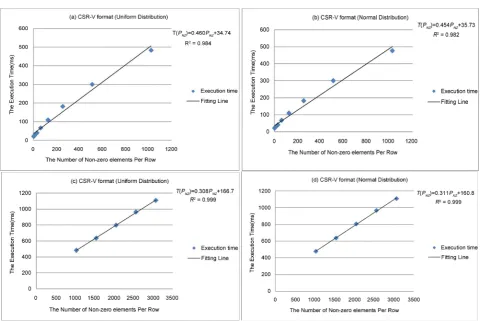
After a large amount of experiments and fitting, we found that for CSR-V ma-trices, the relationship between TB and PNZ is different when PNZ is smaller
or larger than the number of maximum threads per block (1024 for GeForce GTX 540 M). Therefore, the performance fitting function is obtained by the fol-lowing method.
• Establish the function T P
( )
NZFor the benchmark matrices with the same number of strips, we establish the relationship between PNZ and the execution time TB for SpMV. The fitting
functions of two distributions for the number of strips 40 are shown in Figure 1. As can be seen, the relationship between PNZ and TB is approximately linear,
so we make T P
( )
NZ = ×m PNZ+n.• Establish the function E I
( )
For the benchmark matrices with same PNZ, we establish the relationship
between I and the execution time E (i.e. TB in the above) of the
bench-mark matrices for SpMV. The fitting functions of two distributions for PNZ =64 and 2048 are shown in Figure 2. The relation between I and E is also ap-proximately linear, so we make E I
( )
= × +p I q.• Estimate the execution time of a target matrix
For a target matrix, we need to calculate two parameters according to the Eq-uation (6) and D: the number of non-zero elements per row P0 and the number of strips I0, then derive T P
( )
0 and E I( )
0 from above functions, respectively. In order to combat the effects of the difference about functions when the number of non-zero elements per row is smaller or larger than 1024, another execution time t0 of any previously tested benchmark matrix whoseNZ
P is set to be the number of non-zero elements per row in E I
( )
. At this point, estimated execution time of the target matrix in CSR-V format is( )
0( )
0 0
0
T P
T E I
t
Figure 1. The fitting functions of two distributions for I=40 ((a) and (b): PNZ<1024, (c) and (d): PNZ>1024).
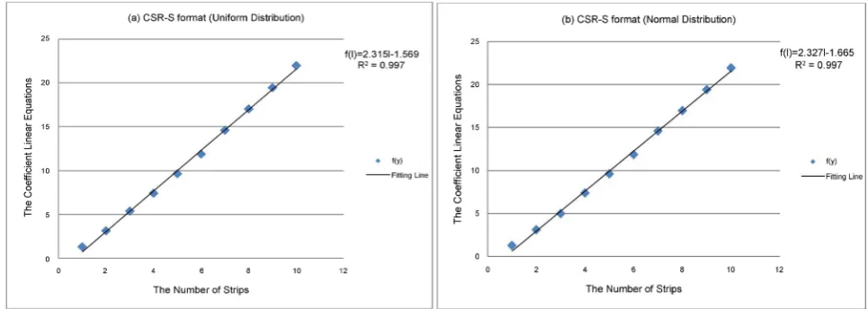
[image:7.595.60.538.419.715.2]3.2.2. CSR-S Format
• Establish the function T P
( )
NZFor the benchmark matrices with the same I , we establish the relationship between PNZand TB for SpMV. The fitting functions of two distributions for
5
I = are shown in Figure 3. As showed in the Figure, the relationship between
NZ
P and TB is approximately linear, so we make T P
( )
NZ = f I( )
1 ×PNZ +g I( )
1 (I1 can be any arbitrary value within the range of I ).• Establish the function f I
( )
For sets of benchmark matrices with different number of strips, we establish the relationship between the number of strips I and the coefficient of the li-near functions f I
( )
in T P( )
NZ . The fitting functions of two distribution areshown in Figure 4. In Figure 4, it is approximately linear between I and
( )
f I , so we make f I
( )
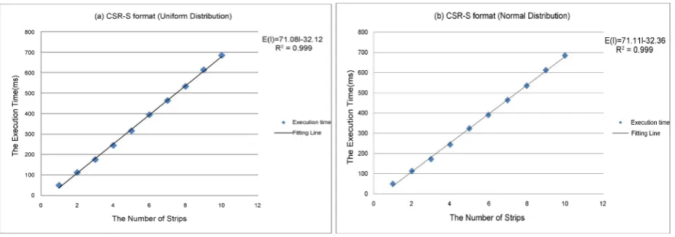
= × +A I B.• Establish the function E I
( )
= f I( )
× +P g I1( )
For Like the fitting function T P
( )
NZ , we establish the relationship betweenthe number of strips I and the execution time E (i.e. TB in the above) of
[image:8.595.63.539.337.508.2]the benchmark matrices with the same number of non-zero elements per row
Figure 3. The fitting functions of two distributions for I=5.
[image:8.595.56.539.541.713.2]1
P, which can be any arbitrary value within the range defined PNZ. The fitting
functions of two distributions for PNZ =32 are shown in Figure 5. We can see that the relationship between I and E is approximately linear, so we make
( )
( )
1( )
E I = f I × +P g I , and the intercept function g I
( )
=E I( )
− f I( )
×P1.• Estimate the execution time of a target matrix
Given a target matrix, we need to calculate two parameters according to the Equation (6) and D: the number of non-zero elements per row P0 and the number of strips I0, then derive f I
( )
0 and g I( )
0 from above functions, respectively. At this moment, estimated execution time of the target matrix in CSR-S format is T P( )
0 = f I( )
0 ×P g I0+( )
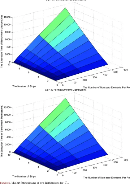
0 .After getting the performance function of CSR-S format, we find that the rela-tionship between dependent variables TB and two variables PNZ, I is saddle
surface in the functional image, that is to say, when I is fixed, the relationship between TB and PNZ is linearity and vice versa, which coincided with the 3D
fitting image we get in Matlab, as shown in Figure 6, which the darker of the colors means the smaller of the values.
3.2.3. ELL and JAD Formats
Note that, the granularity of ELL and JAD format is the same as CSR-S format, which assigns one thread to each row to implement SpMV on GPUs. Therefore, fitting the performance function of ELL and JAD format is done in a similar way with CSR-S format, except the functional expressions. In addition, the 3D im-ages obtained by the Matlab can be fitted with the performance functions and need not be repeated here.
4. Experimental Results and Analyses
[image:9.595.60.541.547.716.2]The experiments are performed on NVIDIA GeForce GTX 540 M with 1 GB global memory, the operating system is a 64-bit Linux with CUDA 6.5 driver. We evaluated our performance prediction model on 30 matrices with each sparse matrix storage format, respectively. These matrices are square real ma-trices from the University of Florida Sparse matrix collection [17]. Moreover,
Figure 6. The 3D fitting images of two distributions for TB.
in order to compare with [16]’s model, we also implement the model in [16] whose PNZ is fixed in benchmark matrices. The estimated time and the
for-mats with three models are given, which is convenient to compare with each other. We define the performance difference rate for different model as
estimated time mesured time mesured time r
D = − (7)
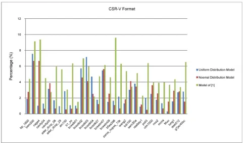
For CSR-V format, the performance difference rate of SpMV in three models of 30 matrices is shown in Figure 7. We can see that Dr in [16]’s model is
5.05% on average, while it is 2.42% and 2.56% for our normal and uniform mod-el, respectively. Compared with the [16]’s modmod-el, the prediction accuracy of the normal model and uniform model are improved by 2.08 times and 1.97 times on average, respectively.
Furthermore, there are three cases for the prediction accuracy of [16]’s model is higher than that of uniform model (such cavity05), and that of normal model (such as bcsstk04). The prediction accuracy of normal distribution model is higher than uniform distribution model for bp_1600 and other 17 matrices.
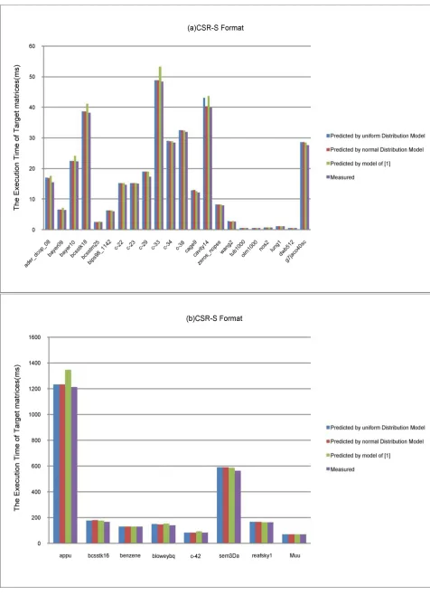
When implement SpMV on GPU with CSR-S format, the performance dif-ference rate in three models of 30 matrices is shown in Figure 8. The average
r
D in [16]’s model, our uniform and normal model is 5.44%, 3.21% and 3.52%, respectively. The average factor for the prediction accuracy of uniform model higher than that of [16]’s model is 1.69, while for normal model, it is 1.54.
[image:11.595.57.539.434.716.2]In addition, the prediction accuracy of [16]’s model is higher than that of normal model on 15 matrices (such as bcsstk16), while for uniform model the better number is 12 (such as bips98_1142). The better number for normal mod-el vs. uniform modmod-el is 13 (such as bayer09) in 30 cases.
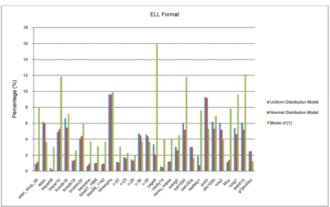
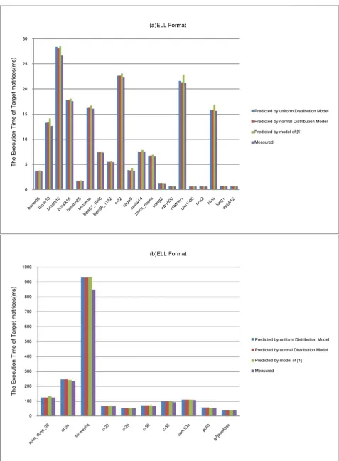
The similar results for ELL matrices are given in Figure 9. It says the average
r
[image:12.595.60.534.106.389.2]D of three models are 5.79%, 3.53% and 3.26%, respectively. The average
Figure 8. The performance difference rate of SpMV on CSR-S matrices.
[image:12.595.57.539.413.715.2]better number for the factor of normal and uniform model vs. [16]’s model are 1.77, 1.64 respectively. The better number for [16]’s model vs. normal model and uniform model is the same 7:23, while for normal model vs. uniform model it is 20:10.
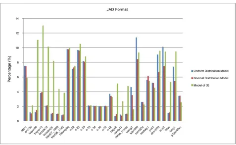
Figure 10 give the results for JAD matrices. Dr of three models are 5.97%,
3.94% and 4.28% on average, respectively. The average improved factor for nor-mal and uniform model over [16]’s model are 1.46 and 1.35. The better number for [16]’s model vs. normal model is 9:21, while for uniform model it is 11:19, while for normal model vs. uniform model it is 16:14.
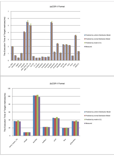
The execution time of four SpMV kernels in three model on 30 matrices is shown in Figures 11-14. There is large difference in the execution time for all matrices in different storage formats. So we put the execution time into two fig-ures: the shorter and the longer in (a) and (b), respectively. Almost all of the es-timated time of the matrices in four different storage formats is greater than the actual measured time. The possible reasons are that we take the number of strips
I by rounding up to an integer.
5. Conclusion and Future Work
[image:13.595.59.537.426.719.2]Aiming at the better performance model of SpMV on GPU based on statistics and [16], we have presented two new models, which consider the structure of matrices. We predict four SpMV CUDA kernels: CSR-V, CSR-S, ELL and JAD. The numerical result shows that the prediction accuracy of our models is higher than that of [16]’s model.
In the future, we will extend our performance prediction model to other SpMV with different storage formats on different kinds of GPUs. In addition, we will propose a new performance model to predict the execution time of a class of iterative methods on heterogeneous parallel machines.
References
[1] Bolz, J., Farmer, I., Grinspun, E. and Schroder, P. (2005) Sparse Matrix Solvers on the GPU: Conjugate Gradients and Multigrid. ACM Transactions on Graphics, 22, 917-924.
[2] Bell, N. and Garland, M. (2009) Implementing Sparse Matrix-Vector Multiplication on Throughput-Oriented Processors. Proceedings of the Conference on High Per-formance Computing Networking, Storage and Analysis, Portland, 14-20 November 2009, Article No. 18. https://doi.org/10.1145/1654059.1654078
[3] Li, R.-P. and Saad, Y. (2013) GPU-Accelerated Preconditioned Iterative Linear Solvers. TheJournal of Supercomputing, 63, 443-466.
https://doi.org/10.1007/s11227-012-0825-3
[4] Vazquez, F., Ortega, G., Fernandez, J.J. and Garzon, E.M. (2010) Improving the Performance of the Sparse Matrix Vector Product with GPUs. Proceedings of the 10th IEEE International Conference on Computer and Information Technology, IEEE Computer Society, Bradford,29 June-1 July 2010, 1146-1151.
[5] Monakov, A., Lokhmotov, A. and Avetisyan, A. (2010) Automatically Tuning Sparse Matrix-Vector Multiplication for GPU Architectures. In: Patt, Y.N., Foglia, P., Duesterwald, E., Faraboschi, P. and Martorell, X., Eds., High Performance Em-bedded Architectures and Compilers. HiPEAC 2010. Lecture Notes in Computer Science, Vol. 5952. Springer, Berlin, Heidelberg, 111-125.
https://doi.org/10.1007/978-3-642-11515-8_10
[6] Zheng, C., Gu, S., Gu, T.-X., Yang, B. and Liu, X.-P. (2014) BiELL: A Bisection ELLPACK Based Storage Format for Optimizing SpMV on GPUs. Journal of Paral-lel and Distributed Computing, 74, 2639-2647.
https://doi.org/10.1016/j.jpdc.2014.03.002
[7] Gu, T.-X., Zheng, C., Gu, S. and Liu, X.-P. (2014) Solving Sparse Linear Systems on GPUs Based on the BiELL Storage Format. Proceedings of International Conference on Parallel, Distributed Systems and Software Engineering, Singapore, 96-107. [8] Choi, J.W., Singh, A. and Vuduc, R.W. (2015) Model-Driven Autotuning of Sparse
Matrix-Vector Multiply on GPUs. ACM SIGPLAN Notices, 45, 115-126.
https://doi.org/10.1145/1837853.1693471
[9] Guo, P., Wang, L.-Q. and Chen, P. (2014) A Performance Modeling and Optimiza-tion Analysis Tool for Sparse Matrix Vector MultiplicaOptimiza-tion on GPUs. IEEE Trans-actions on Parallel and Distributed Systems, 25, 1112-1123.
https://doi.org/10.1109/TPDS.2013.123
[10] Resios, A. (2011) GPU Performance Prediction Using Parametrized Models. Mas-ter’s Thesis, Utrecht University, Utrecht.
[11] Dinkins, S. (2012) A Model for Predicting the Performance of Sparse Matrix Vector Multiply (SpMV) Using Memory Bandwidth Requirements and Data Locality. Master’s Thesis, Colorado State University, Fort Collins.
[13] Baghsorkhi, S.S., Delahaye, M., Gropp, W.D. and Hwu, W.-M.W. (2012) Analytical Performance Prediction for Evaluation and Tuning of GPGPU Applications. Workshop on Exploiting Parallelism Using GPUs and Other Hardware-Assisted Methods (EPHAM’09), in conjunction with the 2009 International Symposium on Code Generation and Optimization (CGO), Seattle, Washington DC.
[14] Hong, S. and Kim, H. (2009) An Analytical Model for a GPU Architecture with Memory-Level and Thread-Level Parallelism Awareness. Proceedings of the 36th Annual International Symposium on Computer Architecture, Austin, 20-24 June 2009, 152-163. https://doi.org/10.1145/1555754.1555775
[15] Schaa, D. and Kaeli, D. (2009) Exploring the Multiple-GPU Design Space. Proceed-ings of the 2009 IEEE International Parallel & Distributed Processing Symposium, Rome, 23-29 May 2009, 1-12. https://doi.org/10.1109/IPDPS.2009.5161068
[16] Guo, P. and Wang, L.-Q. (2012) Accurate CUDA Performance Modeling for Sparse Matrix-Vector Multiplication. Proceeding of the 2012 International Conference on High Performance Computing and Simulation (HPCS), Madrid, 2-6 July 2012, 496-502. https://doi.org/10.1109/HPCSim.2012.6266964
[17] Davis, T. and Hu, Y. (2016) The University of Florida Sparse Matrix Collection.
http://www.cise.ufl.edu/research/sparse/matrices
[18] Nvidia Corporation (2011) NVIDIA CUDA Programming Guide. Santa Clara, Nvi-dia Corporation, USA.
[19] Saad, Y. (2003) Iterative Methods for Sparse Linear Systems. Society for Industrial Applied Mathematics, Philadelphia. https://doi.org/10.1137/1.9780898718003
Submit or recommend next manuscript to SCIRP and we will provide best service for you:
Accepting pre-submission inquiries through Email, Facebook, LinkedIn, Twitter, etc. A wide selection of journals (inclusive of 9 subjects, more than 200 journals)
Providing 24-hour high-quality service User-friendly online submission system Fair and swift peer-review system
Efficient typesetting and proofreading procedure
Display of the result of downloads and visits, as well as the number of cited articles Maximum dissemination of your research work