Development and applications of electrically driven separation methods

Development and applications of electrically driven

separation methods.

BENKE, Peter I.

Available from Sheffield Hallam University Research Archive (SHURA) at:

http://shura.shu.ac.uk/19342/

This document is the author deposited version. You are advised to consult the publisher's version if you wish to cite from it.

Published version

BENKE, Peter I. (2004). Development and applications of electrically driven separation methods. Doctoral, Sheffield Hallam University (United Kingdom)..

Copyright and re-use policy

See http://shura.shu.ac.uk/information.html

Fines are charged at 50p per hour

ProQuest Number: 10694223

All rights reserved

INFORMATION TO ALL USERS

The quality of this reproduction is dependent upon the quality of the copy submitted.

In the unlikely event that the author did not send a com plete manuscript and there are missing pages, these will be noted. Also, if material had to be removed,

a note will indicate the deletion.

uest

ProQuest 10694223

Published by ProQuest LLC(2017). Copyright of the Dissertation is held by the Author.

All rights reserved.

This work is protected against unauthorized copying under Title 17, United States C ode Microform Edition © ProQuest LLC.

ProQuest LLC.

789 East Eisenhower Parkway P.O. Box 1346

Development and Application of Electrically Driven

Separation Methods

Peter I. Benke

A thesis submitted in partial fulfillment of the requirements

of Sheffield Hallam University for the degree of

Doctor of Philosophy

Abstract

Capillary Electrochromatography (CEC) is one of the newest separation techniques. It is a hybrid technique of high performance liquid chromato­ graphy (HPLC) and capillary zone electrophoresis (CZE). It combines the simplest capillary electrophoresis mode where separations are based on the differences in the electrophoretic migration of charged analytes under the influence of a high electric field with separation based on analyte partitioning between the mobile phase and stationery phase from liquid chromatography.

Mass spectrometry (MS), which requires ionized analytes in order to be detected, is an ideal detection technique for CZE. It is also a sensitive, selective and universal detector. However, CZE-MS interfacing is difficult. It is crucial to maintain a stable electrical contact throughout the CE capillary and ion-source as well as adequate grounding of the high voltage applied in CE. The main practical problem is the great mismatch in flow rates through the CE capillary and the solvent flow required for the general LC-MS ion-sources, such as electrospray. Thus, the evaluation of the interfacing is also reported.

The CEC work presented in this thesis details the examination of effects of physicochemical properties of different silica based Cis stationary phases on their chromatographic performance in CEC separations for a series of different acidic, neutral and basic type of analytes.

In the other half of this thesis, the application of a fast electrophoretic separation to improve previous HPLC separation and mass spectrometric detection of surfactants with great importance in oil recovery is reported. The surfactants, commercial nonylphenol ethoxysulphates (NEPOSp) and sulphonates (NEPOS), have been separated by reversed type CZE and the surfactants were also analysed then by mass spectrometric detection on a triple quadruple mass spectrometer using home-built co-axial sheath flow electrospray interfaces.

Acknowledgment

I would like to express my sincere thanks to:

My supervisors, Malcolm Clench and Vikki Carolan, for their help, guidance and full support throughout the course of this study.

My late supervisor, Lee Tetler for his supervision in the beginning of this research.

Boris Duerner and Edward Baidoo for their friendship and help over the years, who stood by me during the difficulties.

My colleagues and staff, especially for Joan Hague, in the Biomedical Research Centre and in the Material Research Institute of the Sheffield Hallam University, both for their advice and making my time in the department more enjoyable.

Declaration

A thesis submitted to Sheffield Hallam University for the degree of Doctor of Philosophy.

All the results and data (otherwise stated) presented in this thesis were obtained by me. No portion of the work referred to in the thesis has been submitted in support of an application for another degree or qualification of this or any other university or other institute of learning.

CONTENTS

Contents...1

Acronyms...5

Symbols and units... 6

CHAPTER 1 - Capillary Electrophoresis... 7

Introduction...8

1 Theory... 10

1.1. Electrophoretic mobility... 10

1.2. Electroosmosis...10

1.3. Electroosmotic Flow... 14

1.4. Analytical parameters in CE...16

1.4.1. Standard deviation... 16

1.4.2. Efficiency... 17

1.4.3. Resolution... 18

1.4.4. Peak Capacity... 19

1.4.5. Selectivity...20

1.4.6. Peak asymmetry... 21

1.5. Dispersion in CE... 22

1.5.1. Flow profile... 22

1.5.2. Band broadening processes...24

1.5.3. The Van Deemter model... 25

1.6. Effect of variables on EOF and analytical parameters... 27

1.6.1. Electric field... 28

1.6.1.1. Voltage...28

1.6.1.2. Capillary Length and Diameter... 29

1.6.2. Temperature...30

1.6.3. pH of the running buffer...33

1.6.4. Concentration and Ionic strength of the Running Buffer...34

1.6.5. Injection plug length...34

1.6.6. Conductivity of the sample (Electrodispersion)...35

1.7. Capillary wall modification (Coatings and Surface modifiers)... 35

1.7.1. Permanent Coatings...37

1.7.2. Dynamic Coatings...39

1.8. Instrumental Considerations...41

1.8.1. Sample injection... 42

1.8.1.1. Hydrodynamic Injection...42

1.8.1.2. Electrokinetic injection...43

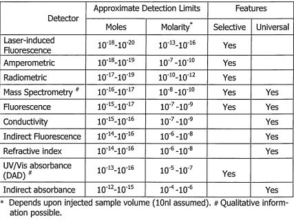
1.8.2. Detection...46

1.8.2.1. Ultraviolet/Visible detection...47

References...53

CHAPTER 2 - Capillary Electrochromatography... 59

2 Capillary Electrochromatography...60

2.1. Introduction...60

2.2. History of CEC...61

2.3. Theory...62

2.3.1. Electroosmotic flow ...62

2.3.2. Separation...65

2.4. Instrumentation... 67

2.5. CEC columns...70

2.5.1 Packed columns...70

2.5.1.1. Frits and Restrictors... 71

2.5.1.2. Packing methods...74

2.5.1.3. Conditioning... 76

2.5.1.4. CEC Stationary Phases...77

2.5.1.5. Mobile phases ... 77

2.5.2. Monolithic columns... 79

2.5.3. Open Tubular columns... 81

2.6. Conclusions... 82

References...84

CHAPTER 3 - Coupling Techniques of Capillary Electrophoresis to Mass spectrometry...90

3 Capillary electrophoresis-Mass spectrometry...91

3.1 Introduction...91

3.2 Liquid-junction interface...92

3.3 Co-axial interface...94

3.3.1 Chemical parameters (Spraying solvents)...96

3.3.2. Physical parameters (Instrumentation)...98

3.4. Sheathless or nanospray interface... 101

3.4.1 Physical parameters of the NanoTips ... 103

3.5. CEC-MS Interface Developments ...104

3.6. Study of CE-MS Nanospray Interfaces...106

3.6.1 Experimental...106

3.6.2 Discussion...108

3.6.3 Conclusions...113

3.6. Summary...114

References...115

CHAPTER 4 - Examination of Ci8 Stationary Phases for the CEC Separation of Acidic, Neutral and Basic Compounds 120 4 Examination of stationary phases... 121

4.1. Introduction...121

4.2. Silica-based stationary phase particles...121

4.3. Stationary phases in CEC... 126

4.5. Experimental...129

4.6. Results and Discussion...132

4.6.1. Physicochemical properties of silica...132

4.6.2. Effect of stationary phase chemistry on the EOF... 135

4.6.3. Chromatographic properties...137

4.6.4. Peak Asymmetry... 138

4.6.5. Efficiency ...140

4.6.6. Retention factor... 141

4.6.7. Column selectivity ...145

4.7. Column Reproducibility... 147

4.8. Conclusions :... 152

References...154

CHAPTER 5 - Separation of Anionic Nonylphenol Ethoxylate Type Surfactant mixtures by CE-MS... 158

5.1. Introduction... 159

5.2. Classification of surfactants...162

5.2.1. Anionic surfactants... 162

5.2.2. Cationic surfactants... 163

5.2.3. Amphoteric surfactants... 164

5.2.4. Non-ionic surfactants...164

5.3. Analysis of surfactants... 165

5.3.1. Anionic surfactants... 165

5.3.2. Cationic surfactants... 168

5.3.3. Non-ionic surfactants...169

5.3.4. Amphoteric surfactants... 171

5.4. Aims of the work... 172

5.5. Experimental...172

5.5.1 Reagents and Materials...172

5.5.2 Equipment ... 173

5.5.3 Sample and Buffer preparation... 173

5.5.4 CE conditions...173

5.5.5 Capillary (pre)treatment...174

5.5.5 Mass Spectrometer conditions...174

5.6. Results and discussion... 175

5.6.1. Nonylphenol ethoxylate sulphonates ans sulphates...175

5.6.2. CE-MS of nonylphenol ethoxylate sulphonates...181

5.6.2.1. Composition of sheath liquid ... 182

5.6.2.2. Sheath liquid flow rate...182

5.6.2.3. Capillary position... 183

5.6.2.4. Applied additional pressure... 184

5.6.2.5. Nebuliser and drying gas flow rate... 186

5.6.2.6. Temperature...186

5.6.2.7. Optimised parameters...186

5.7. CE-MS results... 187

5.8. Conclusions...194

References... 195

Chapter 6 - Conclusions... 197

6.1. Development of a CZE/UV separation of NPEO type surfactants 198 6.2. Analysis of nonylphenol ethoxylate surfactants by CZE/MS...198

6.3. Investigation of stationary phases for CEC...199

6.4. Overall Conclusions... 200

6.5. Future work...201

Acronyms

ACN Acetonitrile

CAPS 3-(cyclohexylamino)-l-propane-sulphonic acid CE Capillary electrophoresis

CEC Capillary electrochromatography CTAB Cetyl trimethyl ammonium bromide CZE Capillary zone electrophoresis DMSO Dimethylsulphoxide

EOF Electroosmotic flow ESI Electrospray ionisation GC Gas chromatography

HEPES N-2-hydroxyethylpiperazine-N'-2-ethanesulphonic acid HDB Hexadimethrine bromide

HPLC High performance/pressure liquid chromatography MES 2-[N-morpholino]-ethanesulphonic acid

MS Mass spectrometry

NPEOS Nonylphenol ethoxylate sulphonates sulphates NPEOSp Nonylphenol ethoxylate sulphates

ODS Octadecyl silane PVA Polyvinyl alcohol

QSSR Quantitative structure-retention relationships TRIS Tris(hydroxymethyl)-amino-methane

SAX Strong anion exchange

SCF Supercritical fluid chromatography sex Stron cation exchange

SDS Sodium dodecylsulphate SEM Scanning electron microscope SIMS Secondary ion mass spectrometry XPS X-ray photoelectron spectroscope

Symbols and Units

N Bonded phase coverage [(imol m'2] a Charge density at the surface of the shear [C cm-2] e Charge per unit surface area [C cm'2] c Concentration (of solution) [g or mol L"1]

K Conductance [Q-1]

I Current _{[A ] ,}

d(p) Density [g cm'3]

dp Diameter of particles Dim]

Sr Dielectric constant of the mobile phase [C2 J'1 m'1]

D Diffusion Coefficient [cm2 s'1]

1 eff Effective capillary length [cm]

N Efficiency (theoretical plate number)

-E Electric field strength [V cm'1]

H ep Electrophoretic mobility [cm2 V s'1]

V ep Electrophoretic velocity [mm s'1]

V EOF Electroosmotic velocity [cm s'1]

F Faraday constant [9.648x1(f C mol'1]

R Gas constant [8.314 J K'1 mol'1]

G Gravitational constant \_6.67xlff11 m3 s'2 kg'1]

I Intensity of light [W m'2]

H- EOF Mobility of electroosmotic flow [cm2 V'1 s'1]

M Molecular weight [g mol'1]

8 Molar absorptivity [L mol'1 cm'1]

A Molar conductance [fl'1 m2 mol'1]

q

£o Permittivity of vacuum [8.85xia12 C2 N 'V 2]

H Plate height [nm] .

R Resistance _[Q]

4>o Surface Potential [mV]

P Pressure [mbar]

r Radius(capillary, particle etc.) [urn]

S Surface area [m2 g'1]

T Temperature _[K]

5 Thickness of the double layer [nm]

L Total length of column [cm] n (dynamic) Viscosity of solution [g cm s' ]

V Voltage [V]

w

5 Zeta potential [mV]

CHAPTER 1

Introduction

Classical electrophoresis is one of the oldest separation techniques. It was developed by Tiselius [1] in 1937 who was later awarded a Nobel prize for his work in separation science. Separation efficiency in free solution, as used by Tiselius, was limited by the thermal diffusion caused by Joule heating and convection. For this reason, classical electrophoresis is traditionally performed in an anti-convective support media such as gels [3]. This form of electrophoresis is still used for separation of biological macromolecules, despite the efficiency and sensitivity problems and long analysis times observed.

The use of narrow tubes allowed open tube electrophoresis of free solutions to be studied, but many problems were encountered. Kolin developed rotating tube electrophoresis in 1954 [2] to reduce unwanted convection. Initial work in open tube electrophoresis, firstly using capillaries, with the minimum 1mm internal diameter available that time, was described by Hjerten in 1967 [3]. He also used rotation (along the longitudinal axis of the capillaries) to reduce convection effects. In the 70's Virtanen [5] and then Mikkers [4] used smaller (ID=~200jim) glass and Teflon capillaries to demonstrate the advantage of capillaries over narrow bore columns in electrophoresis.

Historically, Isotachophoresis (ITP) is very important in the development of modern CE. It was used as early as in 1970 by Everaerts and his group [6] to separate organic acids. ITP was the most widely used CE technique prior the 80's and the principles and practicalities learned were used later in Capillary Zone Electrophoresis (CZE).

using 75pm fused silica capillaries. Several new techniques, utilising electrophoretic effects in capillaries were developed at that time:

• Micellar electrokinetic chromatography (MEKC) a technique for the separation of non-ionic species, which do not migrate in an electric field, was developed in 1984Terabe etal. [9,10];

• Isoelectric focusing (CIEF) [11,12] by Hjerten in 1985

• Gel electrophoresis (CEG) for the size-based separation of macromolecules by Cohen and Karger in 1987 [13,14]

• Column-transient Isotachophoresis (CUP) by Karger and Foret in 1992 [15,16].

The last CE technique (of which first application can be traced back ironically to the time of birth of the CE technique itself, when Strain applied electric field across in an absorption column in 1939 [17]) to be developed, is the combination of HPLC and CE, Capillary Electrochromatography (CEC). The potential of this technique was first demonstrated by Jorgenson and Lukacs in 1981 [7,8], using fused silica capillaries similar to those employed in GC, but it took another 10 years when Knox and Grant confirmed their theoretical work in 1991 [18,19], before the resurrection of the CEC technique and it's worldwide application really started. In the last decade, several groups have made contributions [20,25] to the development of CEC, and this is a process, which is ongoing.

Instruments for CE have been commercially available since 1988. At the beginning the precision of these instruments was too poor for quantitative analyses. The worldwide spread of the application of CE started after 1993 when precision reached 1-2% RSD for peak areas and heights for the available instruments [26] and the experience of validation of the CE methods and instruments had grown [27].

1

Theory

1.1 Electrophoretic mobility

Electrophoresis is the movement of electrically charged species towards the oppositely charged electrodes in a conductive media (electrolyte) under the influence of an electric field. In capillary zone electrophoresis, separation is based on an ion's electrophoretic mobility (pe)- The rates and directions of migrations of a spherical ion are the function of the charge-to-size ratio of the ions and the signs of their charges [28,29].

r.= -r~

(i-i)

q - Number of charges on an ion; rj = Buffer viscosity; r - Ion radius

The electrophoretic velocity of an ion (ve) is directly proportional to the electric field (E) across the system

l l 2 )

E ' l <’ -3)

V - Voltage, L = Total length of the capillary.

Thus, the smaller and/or multivalent ions are moving faster than the big and/or monovalent ions, while the neutral molecules are not influenced by the electric field and they only move together with the conductive media, therefore they cannot be separated from each other.

1.2 Electroosmosis

field due to the electroosmosis, which is the basis of the possibility of separation between positive and negative ions.

When an electrolyte solution is placed into a fused silica, an electric double layer is created at the interface between solid and liquid phases [30-32]. The inner wall of fused-silica capillary is negatively charged due to the presence

Cathode

Capillary wall

Plane of shear

£

<

<

<s

<

<

<

0 G 0 G +o q G

@@ ©©

9 9

99

|-° ® ©

-o © ©

"0 ® ©

-o © ©

G ®

G© -o G@ G 0 G 0 to 0

%

G

G

ft

-o

G G G 0 0 G ft G G | 0 G

0 0 0 G 0

© ® ©

© 9

0 G G

® @©

G G G 0 0

G G ^ @ G 0

G 0

Fixed

layer Mobile layer

Diffuse double layer

O

0

0

©

©

0

©

0 0

I

I

Bulk solution

Anode

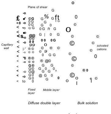
Figure 1.1 Representation of electric double layer at the fused silica surface of the capillary.

of weakly acidic silanol groups (pKg 2.2) which dissociate to silanolate groups (=Si-CT) above pH=2. Positive ions in solution gather near the capillary

surface to balance this negative charge, giving rise to an electric double layer (Figure 1.1).

The electric double layer contains a compact ion-binding region, the Stern or fixed layer, and a diffuse layer, or Gouy-Chapman layer [33,34]. The reason for the formation of the diffuse layer is that the fixed layer is not able to neutralise the surface's negative charge, due to steric hindrance. The excess cations that are firmly held in the Stern layer, close to the capillary surface are believed to be less hydrated than those in the diffuse region [35]. The cations in the Gouy-Chapman layer are more diffuse, hence the name, and able to move into the bulk solution and back. The plane where the diffuse layer begins is called the outer Helmholtz plane, and the edge for the compact region of bound cations is called the inner Helmholtz plane [33].

The potential at the fused-silica capillary wall is proportional to the charge density resulting from the dissociation of the silanol groups. The potential decreases linearly from the wall potential (<|)o) to the Stern potential (<^) in the Stern layer, and then exponentially from ^ to zero in the diffuse layer (Figure 1.2).

Plane of shear

Charge density

- z/8

G =

Stern

layer Gouy-Chapmanlayer

Fixed

layer Mobilelayer

Distance z

Figure 1.2 Diagram of charge density in the electric double layer.

The zeta potential is influenced by the dissociation of the silanol groups at the fused-silica capillary wall, the charge density in the Stern layer and the thickness of the diffuse layer. Each of these parameters depends on several variables, such as pH, specific adsorption of ions in the Stern layer and ionic strength of the electrolyte solution. The dielectric constant, viscosity and nature of the solvent also all have an effect on the zeta potential [36].

S = Thickness of diffuse double layer; e = Dielectric constant of the buffer;

e = Charge per unit surface area.

The thickness of the double layer is inversely proportional to buffer concentration.

eo = Permittivity of a vacuum; sr = Relative dielectric constant of the buffer

solution; R = Gas constant; T- Temperature; c = Concentration of the electrolyte; F - Faraday constant.

For binary electrolytes in aqueous solution, the double layer thickness of electrolytes with concentrations of 10*6 to 10'2 M ranges from 3 to 300 nm [37]. A 10 mM buffer producing an approximately 1 nm thick double layer [38]. Under an electric field, the thickness of the diffuse layer is indirectly proportional to the square root of the ionic strength of the electrolyte solution [32,35]

The pH of the solution has a major effect on the zeta potential. An increase in solution pH directly influences the charge density on the capillary wall [34,39] due to increasing deprotonation of the surface silanol groups. Zeta potentials of a silica surface in a typical aqueous CE media are in the range of 1-100 mV [40,41]

£ (1.4)

(1.5)

1.3 Electroosmotic Flow

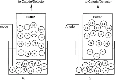
If an electric field is applied across the fused-silica capillary the cations in the fixed layer stay tightly held, but the cations in the diffuse layer can migrate towards the cathode, dragging their solvation spheres with them. Since the water molecules associated with the cations are in direct contact with the bulk solution, all the electrolyte solution moves towards the cathode. This flow is called the electroosmotic flow (EOF).

The magnitude and direction of the EOF are controlled by the zeta potential, and can be described by the Helmholtz and Smoluchowski equation [28,29]

Me o f ~ A_Anij

(1.6)

H eof = Electroosmotic mobility; s = Dielectric constant of the solution; £ =

the zeta potential and r\ = Viscosity of the solution.

The electroosmotic mobility is analogous to electrophoretic mobility, both have the same units, [cmVV's]. The same applies to electroosmotic velocity, which can be calculated on the same basis as Eq. 1.2. The observed velocity, vobs, of an ion is influenced by its electroosmotic velocity and mobility and the velocity and mobility of the running buffer (EOF)

V o t , = V E O F + (L 7 )

from Equation 1.2

V obs ~ ( M e MeO F ^ ^ (

1

8

The observed velocity of the EOF can be easily calculated using a neutral analyte, the so called neutral marker, which moves together with the EOF, by measuring migration time (or retention time), tmarker:

_ l«

V0bs— (1>9)

leff = Effective capillary length (from the point of injection to the point of detection).

The migration time for an ion can be obtained from:

t = l "L (

1

10

(M e Me o f

The calculation of the electrophoretic velocity of an ion is possible from its migration time, tm, by rearranging Eq. 1.7 and substituting into Eq. 1.9 to give:

_ l eff Le ff

e~~t T ~_{m marker} ( i . i i )

The electrophoretic velocity can be calculated from experimental parameters (rearranging Eq. 1.8 after substitution of eqs. 1.3,1.7 and 1.9) using:

M e =

( I L \_{l e f f ^} tmV

\ m J [ t ^ r V JEOF

(

1

12

As can be seen from the above equations, the separation of differently charged and neutral species (but not between the neutral species) is possible.

Under normal conditions of CE (when the negatively charged electrode is at the same side as the detector, and the EOF move towards the outlet vial) the migration order, from equation 1.8, will be as follows:

• Cations migrate first, before the EOF as their electrophoretic mobilities add to the mobility of the EOF.

• Neutral species migrate at the same rate as the EOF as the electric field has no effect on them.

• Despite the opposite direction of the electrophoretic migration of the anions, the EOF of the buffer solutions (p e o f) is usually greater than their

electrophoretic mobility. Thus, anions are carried along behind the EOF and they migrate last.

The migration order of ions with the same charge is based on their charge-to-size ratio, as described in Section 1.1.

1.4 Analytical parameters in CE

The quality of a separation method is described by efficiency, resolution and analysis (migration/retention) time. Further parameters such as peak asymmetry and selectivity also give useful information about the analytical performance of the techniques. The main advantage of capillary electrophoresis is that much higher efficiencies can be obtained in analyses, as will be explained.

1.4.1 Standard deviation

In chromatography moving solutes disperse into a diffuse band and this is detected as a Gaussian peak with standard deviation (a) due to differences in the analyte velocity within the solute zone. The resultant peak width at the baseline (w) can be expressed as

w = 4cr

(1.13) If the dispersion arises only from diffusion (which is the main cause of broadening), the standard deviation of a solute zone is

<7 = V557

(1.14) D = Diffusion coefficient of the analyte; t = migration time

Under ideal conditions in CE, the only diffusion is longitudinal as radial diffusion is negligible due to the flat flow profile.

variance (a2). Eq. 1.14 can be written after substituting migration time (Eq. 1.10) as

0.2 _

( M ' + M e o fW ( L 1 5 )

1.4.2 Efficiency

Efficiency (N) relates the analyte zone (peak) width to the distance it travelled during the separation in the system and is expressed as the number of theoretical plates (the name originates from distillation procedure theory, firstly presented by Martin and Synge (1941) and G/ueckauf (1949))

N = 1 6 x

( t V

tR = Migration time; w = peak width at the baseline

The number of theoretical plates can be related to the variance as

N = ( L \ 2 L_

H

H = Height equivalent to a theoretical plate; L = Length of column

(1.16)

(1.17)

The maximum separation efficiency of a CE system in ideal conditions, where only longitudinal diffusion contributes to brand broadening, can be derived from 1.14 and 1.10

^ = MgppV

2D _(1.18)

As diffusion is the most important factor causing brand broadening the shorter the separation time the higher the efficiency as the analytes spend less time in the capillary and therefore they have less chance to diffuse. Thus equation 1.18 illustrates one very important aspect of CE that efficiency is not based on the length of the capillary used and therefore short capillaries can be used, which means faster separations. This is in contradiction to

liquid and gas chromatography, where longer columns give higher efficiencies.

In CE high efficiency can be achieved by the application of a higher voltage (see Section 1.5.1.1-1.5.1.2), which leads to higher EOF.

1.4.3 Resolution

The most important separation parameter, the resolution (R) between two adjacent peaks is defined as the difference in migration times (t) related to the peak width:

^ _ At _ 2 ~^1 )

w w1+ w2 ( L ig )

w = average peak width at the baseline; At = separation time difference

Baseline separation is achieved for two peaks with the same area when the resolution is 1.5. When resolution is 1.0 the overlap is 2.3% and the separation time difference between the peak tops is 4a [42]. Resolution can be related to efficiency [28] as

4 v

(1.20)

Av = velocity difference between two peaks; v = average velocity of the two analytes

It can be also expressed with electrophoretic parameters as

R = 0.177 (1.21)

(f j, + f ip Q f ) ”V D

As can be seen, increasing the efficiency will result in less improvement in resolution than increasing the difference in the electrophoretic mobility of the analytes. Maximum resolution can be obtained when the average electrophoretic mobility of the analytes is equal to the EOF but in opposite direction. Although, the migration time is at maximum in this case due to Eq. 1.10.

Optimising the mobility difference between the analytes {e.g. controlling the pH, application of proper running buffer and/or organic solvents) is the main approach for achieving good resolution.

1.4.4 Peak Capacity

The separation capabilities of different techniques can be compared by the peak capacity (Cp or P). This gives information about the "ideal", maximum number of peaks that can be resolved in a given system and specified time, when the resolution between consecutive peaks is 1.0.

CP =1 + — lni - = l + — ln(l + *)

4 4 v '

(

1

22

tr = Migration (retention) time of the analyte; tnm = Migration (retention) time of a neutral marker or an unretained sample; k= retention factor.

The lower limit of peak capacity is the dead time of the system - the time of the mobile phase passes through the system - which is equivalent with W The practical maximum limit - due to the finite peak width as defined by the

plate number - is when t r/tnm is 10 in most LC and 50 in many GC

1.4.5 S

electivity

The selectivity (a) of a chromatographic system describes the separation level that can be achieved between two adjacent analytes based on their selective retention by the stationary phase (in CEC, for example). It is expressed as the distance at the peak apex between two consecutive analyte peaks:

a = -2-~ tnm

u - tnm

(1.23) ti , t2 = Migration times of the analytes; tnm = Migration time of a neutral marker.

Substituting Eq. 1.2 and 1.11 into the selectivity equation, the selectivity can be related to electrophoretic mobility (p) of the analytes

M i

a = — x const

M i

(1.24) As can be seen, selectivity can be improved by changing the difference between the electrophoretic mobilities of the analytes {e.g. altering the pH, see 1.6.3)

In partition chromatography {e.g. LC, CEC) the selectivity can be described as a function of the retention of each component by the stationary phase

k0

a ~ K (1.25)

Where k is the retention or formerly capacity factor. It describes the retention properties of the stationary phase, the ratio of the total number of molecules in the stationary and mobile phases. It can be calculated with regard to the migration times:

The dead time is the time for the mobile phase reaches to the detector throughout the system. In CE this can be related to the migration time of a neutral marker (tnm), which moves at the same velocity as the running buffer in the capillary and is unretained on the stationary phase in the case of CEC.

1.4.6 Peak Asymmetry

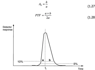
Peak Asymmetry (As) and Peak Tailing Factor (PTF) describe the deviation of the resulting peak shape from a perfect Gaussian distribution. Peak asymmetry is calculated as shown in Figure 1.3, at one-tenth of the maximum peak height, while tailing factor is calculated at 5% of the maximum peak height [44]

As ~

PTF = a + b

2 a

(1.27)

(1.28)

Detector response

10%

5%

t,r Time

Figure 1.3 Determination of peak width fractions for peak asymmetry and tailing.

A peak asymmetry value of 1.0 indicates symmetrical peaks, whereas higher values indicate "tailing" peaks and lower values indicate "fronting" peaks.

These measurements of the peak shape are important indicator values of chromatographic problems such as

- analyte-capillary wall/stationary phase interactions (absorption) causing peak tailing

- sample overloading causing peak fronting

- mismatch in sample and running buffer conductivities (electrodispersion) causing tailing or fronting

It should be noted that strictly - as the plate theory is based on symmetrical Gaussian peaks - parameters such as efficiency become more complex if asymmetry occurs. An approximate calculation, the Dorsey-Foley equation, can be used for plate numbers in the case of asymmetric peaks [42]

r

4 1 . 7 x

a + b

— + 1 . 2 5

a

(1.29) tr = retention time; a and b = the peak width fractions at one-tenth-height as in Figure 1.3.

However, asymmetry values up to 1.25 are considered as indicating acceptable peak shapes in HPLC methods and the analytical parameters are calculated as normally.

1.5 Dispersion in CE

1.5.1 Flow profile

velocity is reduced directly at the capillary wall due to frictional forces, its effect is negligible compared to the total flow profile. The overall result is a relatively flat flow profile (Figure 1.4).

This is the opposite to pressure driven systems (such as LC, GC) which have a laminar (HPLC) or turbulent (GC) flow, with parabolic flow profile due to the frictional forces which creates different flow velocities across the column/capillary.

Electroosmotic flow

Plug flow

=>

resultant peak

Pumped flow

Laminar flow

Figure 1.4 Comparison of electrically and hydrodynamically driven flow profiles and their resulted peaks

The flat flow profile of the electrically driven systems not only occurs in open tubes, but in packed capillaries as used in CEC as well (Figure 1.5). Although, the generation of the flow is mainly connected to the surface of the stationary phase particles in CEC (see Chapter 2.1), the generation of the EOF is the same.

CEC HPLC

=>

a

a

Q

a

Figure 1.5 Comparison of flow profiles through a stationary phase in CEC and HPLC.

Despite the several flow channels in the stationary phase among the particles, the EOF is uniformly distributed along the whole stationary phase, thus the same plug flow produced throughout each channel and the whole capillary, with an overall flat flow profile.

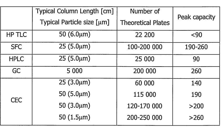
The result is that all analytes will move with the same velocity and hence peak broadening is minimal in CE systems. Therefore narrower peaks with very high efficiencies and better separations can be obtained compared to pressure driven systems (Table 1.1).

Technique N [plates/m] TLC <5000

GC 3000

SCF 260 000

HPLC 100 000

CEC 250 000

CZE 4 000 000

Table 1.1 Comparison of the most common separation techniques [28]

1.5.2 Band broadening processes

The reachable efficiency in a practical application (measured by Eq. 1.16) is generally smaller than the theoretically calculated one (Eq. 1.18), due to the presence of several dispersive processes other than the longitudinal diffusion. The total dispersion in an analytical system can be described by accounting for all possible dispersive processes which contribute to the variance of the final band broadening:

2 2 2 2 2 2 2 2

®observed / j® i . ® D iffusion ^Electrodipersion ^ In je c tio n ®Tem peralue ® Adsoption ^D ete ctio n

1.5.3 Th

e Van Deemter model

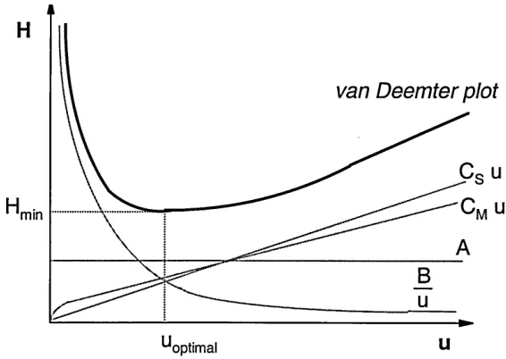
To improve the separating performance of a chromatographic system, the original plate number theory is not adequate as it is not related to the real physical and chemical processes taking place in a practical column/capillary. It was van Deemter etaL [45] who described a general equation to describe the band broadening processes in practical chromatographic separations, relating the plate height (H) to the linear velocity (u) of the mobile phase through the column. Later several corrections were published to improve the van Deemter equation [46-47]

H — A H f- (Cs + CM)u

u

(1.31) A, B and C coefficients are constants for a particular analyte and experimental condition as the flow rate is varied. They describe different band broadening processes.

van Deemter plot

'min

^optimal U

Figure 1.6 Hypothetical van Deemter plot showing the relative contribution of different components into the total plate height

solutes take during migration through a packed column. This results in different speeds for each solute as they migrate through different lengths of the packed bed during the separation. The A-term in CEC is generally less than in HPLC for any particular particle size as individual flow velocities in the different flow channels are the same due to EOF, as described in Section 1.5.1. The value of A can be reduced, thus less band broadening can be achieved by using smaller particles with a smaller size distribution. This generally improves the homogeneity of the packing. Unlike in HPLC, there is no pressure limit in electrochromatography, thus the use of much smaller particles are possible. The A term only depends on the packing geometry (density and homogeneity) of the stationary phase, and is independent of flow rate.

The B term (Molecular diffusion) is related to the concentration gradients between the sample plug and the surrounding mobile phase. This concentration gradient causes molecular diffusion in all directions independently from the flow direction. The longitudinal diffusion - along the axis of the column - will result an axial sample zone spreading. The diffusion rate is proportional to the component's diffusion coefficient and temperature (section 1.4.1). It is also depends on the time the solute spends in the column and is thus inversely proportional to the flow rate. Therefore the higher the velocity the less the diffusion occurs.

The EOF offers no advantage over pressure driven systems for the reduction of molecular diffusion. This is the main band-broadening factor in electrophoretical separations under ideal conditions.

example will stay in the stationary phase while others moved further, causing tailing.

The C term is often used in a combined form, but it can be described by two separate coefficients. The Cs term describes the diffusion in the stationary phase and Cm in the mobile phase. Both factors are dependent on the

diffusion coefficient in the given phase. Further more Cs is related to the stationary phase film thickness, while CM is related to the particle diameter and can be reduced by using smaller particles. The effect of Cs can be largely ignored as the mass transfer of the analyte onto and off of the stationary phase is a very rapid process.

The C term is directly proportional to the flow rate. The slower the flow, the more complete the equilibration can be, thus less band broadening occurs.

1.6 Effect of variables on electroosmotic flow and analytical parameters

To obtain a good separation by CE a stable and constant EOF is very important. In some techniques inhibition of the EOF is required {i.e. capillary isotachophoresis, isoelectric focusing and capillary gel electrophoresis).

It should be noted that the effect of the variables that will be described can be multi-fold {e.g. influencing the dispersion and other parameters as well) and that they can work in opposition for or support of other variables. Thus increasing or decreasing the effects of each other. Thus the optimisation of the system is very important.

The basis of EOF control, the effect of different variables will be described briefly.

1.6.1 El

ectric field

The electric field can be changed by the applied voltage or the total length of the capillary (Eq. 1.3).

1.6.1.1 Voltage

As shown by Eq. 1.2-1.3, increasing the voltage will increase the EOF. This results in shorter migration times, thus faster separation, and higher efficiencies. This suggests the use of the maximum voltage possible. The maximum available voltage is ±30kV in most commercial instruments. Unfortunately, higher voltages will result in higher current and the generation of Joule heat. The effects of the temperature will be described in Section

1= Current

The relationship between the current and voltage is described by Ohm's law

R= the resistance of the system, which is related to the buffer electrolyte and the parameters of the capillary. This can be calculated as

A = Molar conductivity of the buffer; C- Concentration of the buffer; Z=Total length of the capillary; d= Diameter of the capillary.

By combining Eqs. 1.32-1.34, the rate of heat generated can be expressed as

1

.

.

.

The heat generated is proportional to the power, P,

P = VI (1.32)

V = IR (1.33)

4AZC (1.34)

The optimal maximum voltage can be determined by plotting, E versus V (Ohm's plot). The relationship between the applied voltage and the generated current is linear until excessive heat is not generated. When this happens the resistance will rapidly decrease, causing a rapid increase in the current [27]. The maximum voltage that should be used is the voltage at the end of the linearity in the Ohm's plot.

The maximum voltage depends on the buffer's concentration, composition and pH, as well as the capillary length and diameter (as can be seen in Eqs. 1.34-1.35)

1.6.1.2 Capillary Length and Diameter

Reducing the capillary length, if the voltage is kept constant, will reduce the resistance of the system (Eq. 1.34) and consequently will increase the generated current and heat. That means that shorter capillaries have lower optimum maximum voltage.

Changes in the diameter have the opposite effect, due to the increased resistance in narrower capillaries. The maximum diameter for CE was reported to be 200pm, as above this it is not possible to effectively dissipate the heat [48].

produced heat. The resolution, on the other hand, is better for longer capillaries, but the analysis time is also longer. As can be seen, just from this section, CE optimisation can be difficult as the variable parameters and their effects are all connected.

1.6.2 Temperature

Temperature has various problematic effects in a CE system. Some of them have been explained in the previous section.

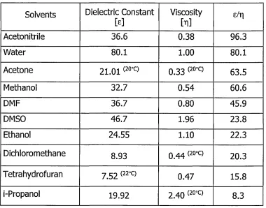
The effect of the temperature on EOF is complicated as it is influenced by two factors, the viscosity and dielectric constant of the buffer, which work against each other. These have an opposite effect on the EOF as can be seen in Eq. 1.6. The final effect of the temperature depends on the composition of the buffer and its e/rj ratio. Table 1.2 (at 25°C unless otherwise indicated).

Solvents Dielectric Constant

[e] ViscosityM s/r|

Acetonitrile 36.6 0.38 96.3

Water 80.1 1.00 80.1

Acetone _{21.01 (20°C) 0.33 (20°c) 63.5}

Methanol 32.7 0.54 60.6

DMF 36.7 0.80 45.9

DMSO 46.7 1.96 23.8

Ethanol 24.55 1.10 22.3

Dichloromethane _8.93 q 4 4 (20°C) _20.3

Tetrahydrofuran _{7.52 (22°c) 0.47 15.8}

i-Propanol _{19.92 2.40 (20°C) 8.3}

Increasing the temperature will decrease the value of both of these constants. A 1 degree Celsius change in temperature can result in a 2-3% change of viscosity (water: 2.4%), and consequently the same change in mobility [50]. The same change results in less change in the dielectric constant of water (0.5%) [27]. Therefore the overall effect for water will be an increase in EOF.

The main problem that can be caused by the generation of excess heat is when the temperature is high enough in the buffer or solute zone for boiling. This results in bubble formation. Sample decomposition or denaturation may occur as well. Such bubbles not only produce separation and detection problems {e.g. false peaks), but they can stop the EOF. Since air bubbles are not conductive, the electrical contact through out the system is broken and therefore there is no electrical field. If the method used is not open-tubular, the bubbles can damage the packed media in the capillary. This is a major problem, especially in CEC, where the formation of a good packed capillary is still a major difficulty. If bubble formation occurs, the system must be flushed out with the running buffer. This can be done easily in CZE, but not in CEC.

The heat generated can result in temperature and density gradients and subsequent convection. These temperature gradients can damage the separation, due to zone broadening and unreproducible migration times (section 1.5) [51]. The temperature in the centre of the capillary is higher than that at the edges, producing a parabolic flow profile within the capillary. Joule heating can be controlled by operating at a voltage where the heat can be effectively dispersed [51]. However, theoretical calculations have suggested that, a 1.5°C centre-to-wall temperature difference in aqueous electrolyte will not cause a serious decrease in the plate numbers of the system for thermostated capillaries with an inner radius < 50 pm [52].

Capillary

Polyimide ' coating

Centre Wall Wall

Temperature

Surrounding environment Surrounding

environment

25 375 390

25 0 390 375

Distance [pm] Figure 1.7 Schematic of temperature gradients in a CE capillary and around it.

Dissipation of heat through the walls, causing a thermal gradient between the capillary centre and the surrounding environment is shown schematically in Figure 1.7 [53].

The application of longer capillaries with narrower inner radius and larger outer diameter is advantageous due to the better heat dissipation to the

10

.72

8

6

5.58

4

3.14 1.39

2

0.53

0

0 10 20 30 40 50 60 70 80 90 100 110 120 130 140 150

r Om]

Figure 1.8 Graphical example of the calculated centre-to-wall temperature difference for capillaries with different radius (based on [52])

surrounding environment as the insulating effects of the polyimide coating is reduced.

However, the analysis time can be reduced at higher temperature and in some cases enhanced resolution can be obtained or can be used to affect protein conformation [54,55].

Despite these positive effects, the problems caused by the excess heat are generally much greater. Therefore temperature is usually not an operational variable in method development and CE systems are generally thermostated with high velocity airflow, to reduce the generated heat and maintain a constant temperature (± 0.1°C) through the analyses.

1.6.3 pH of the running buffer

The pH is the most crucial parameter in CE. It has a significant effect on the generation of EOF, since it changes the zeta potential through its influence on the deprotonation of the inner surface of the capillary. The pH dependence of the EOF for different capillary materials has been discussed by Lukacs and Jorgenson [49].

The pH also influences the analytes' electrophoretic mobility due to the changes in the degree of ionisation.

The effective mobility, peff, of a monovalent weak acid or base is determined

by _{^ eff= f i ea}

(1.36)

a = the degree of dissociation, given for a monovalent acid by

1

a ~ (l+\0pKa~pH) (1.37)

and for a monovalent base by

1

a ~ {\+\0pH-pKa) (1.38)

pKa =the acid constant.

The charge and, thus, the electrophoretic mobility of an ion are affected by the pH of the electrolyte solution [38]. Thus, altering the pH a general step in method development.

1.6.4. Concentration and Ionic strength of the Running Buffer

The EOF is reduced at constant temperature, if the ionic strength or concentration of the buffer is increased. The reason is the reduced zeta potential since the increased ionic strength compresses the diffuse double layer, and decreases its thickness (Eq. 1.5).

Reducing the buffer concentration too much, to obtain a high EOF, can cause asymmetric peaks and band broadening. The conductivity can be different in the running buffer and the sample plug and this can cause distortion in the electric field. (The ionic strength of inorganic buffers is usually higher than that of the organic buffers at the same concentration. Therefore, this must be take account when choosing a buffer for a given pH range).

1.6.5 Injection plug length

During injection it is important to minimise the sample plug length as the resolution and efficiency is diminished if it is longer than the dispersion caused by diffusion (see 1.5).

W ■

_ 2 nj

<7 Inj = 12

(

To minimise the injection contributions to the loss in efficiency, the injected plug length should be as short as possible. It is recommended that it should be less than 1-2% of the total capillary length [51,56]. This is equivalent to less than a few tens of nanolitre of sample [6-70nl] or 3-16mm plug length for generally used capillaries (L=30-80cm, I.D.=50 and 75 jum)

1.6.6 Conductivity of the sample (Electrodispersion)

The conductivity of the sample and the running buffer should be similar to avoid peak distortions caused by electrodispersion. Since the conductivity is inversely proportional to electric field strength, the electric field will be lower outside the sample zone if the running buffer has a higher conductivity than the sample. Thus, when an analyte diffuses into the buffer from the back of the sample zone it meets a lower electric field and its velocity is reduced. As the sample zone moves away, peak tailing also occurs. If the analyte diffuses into the buffer from the sample zone front, its velocity will also be reduced. But as the zone reaches this slower analyte it can diffuse back into the sample zone. This keeps the sample front sharp. The overall result will be a skewed, triangular shape peak, which can lead to loss of resolution.

To minimise band broadening the conductivity of the sample should match with the running buffer or the sample concentration should be much less (approximately one hundred times) than the concentration of the running buffer.

1.7 Capillary wall modification (Coatings and Surface modifiers)

magnitude of the EOF becomes unpredictable leading to poor repeatability of mobilities of analytes.

In particular proteins have the unfortunate property of sticking to the capillary wall due to multi-modal interactions, such as hydrophobic, hydrophilic, electrostatic, hydrogen bonding and van der Waals interactions [59]. The adsorption of the analytes reduces the separation performance due to peak broadening and tailing resulting in decreased efficiency or even the analytes total retention on the inner surface.

Capillary conditioning (pre-treatment and regeneration of the inner surface) for fused-silica is commonly used to overcome this problem. Before the application of a new silica capillary, it is generally washed through with alkaline solution - typically 1M Sodium hydroxide solution - then with water and finally with the running buffer. This procedure will ensure the full deprotonation, and uniform charge of the inner capillary wall. The regeneration of the charged capillary surface is often required between sample runs, to overcome the problem of analyte-wall interaction, or migration instability. The regeneration step applies the same procedure, but with less concentrated alkaline media (0.1M) as the silica surface can be damaged by strong alkalis, since the silica is soluble in strong bases. At pH greater than 11, dissolution of the silica capillary material becomes on issue.

Simple rinsing between the runs, with the running buffer, was also reported to help reproducibility [57]. It must be noted that capillary reconditioning with alkalines cannot be used with most of the coated capillaries and with packed CEC capillaries, as it may damage the modified inner surface or the stationary phase particles.

in the running buffer) [58,59]. Both modification methods have advantages and disadvantages.

The use of extreme pH can make capillary wall derivatisation unnecessary, although in the case of protein analysis care should be taken using such pH. Outside of their physiological conditions protein structure may be irreversibly altered, aggregation and/or unfolding may occur and biological activity may become very different.

1.7.1 Permanent Coatings

The EOF can be suppressed or controlled at a certain pH, and analyte-wall interactions can be reduced or eliminated, by coating the active sites on the inner surface of the fused-silica capillary. The active sites contain unreactive siloxane bridges, hydrogen bonding sites and ionisable vicinal, geminal and isolated silanol groups [35,44]. The structure of the silica surface will be more fully discussed in Chapter 4.

Several approaches have been tried for the preparation of permanent coatings. These can be divided into two types: (1) coatings that are covalently attached to the capillary surface; (2) coatings that are adsorbed to the surface by physical or ionic forces, which however, unlike dynamic coating are not dissolved in the running buffer during the separation [53,58,59].

This can be overcome by direct Si-C-R coupling. The direct Si-C bond can be formed by the use of a Grignard reagent. These coatings were reported to be stable between pH=2-10 [63]. However, these processes are difficult and time-consuming and the coating may not be reproducible as a result [64].

Single step procedures were described by Zhao et a/. [65]. First a static coating (using Poly(ethylene glycol), PEG) is formed on the surface, then after the evaporation of the volatile solution, the permanent coating is formed by heating.

To achieve a homogeneous coating surface, the capillary wall must be cleaned and activated prior to the coating process in a similar way to capillary conditioning. This rinsing procedure includes etching with sodium hydroxide to remove impurities from the fused-silica capillary surface, and leaching with hydrochloric acid to remove trace metals. [58]

The adsorbed coatings are prepared by flushing the capillary through with the reagent in a suitable electrolyte solution. The hydroxylic polymers usually require thermal fixation (to cross-link between the polymer chains) to become stable. Before the analysis, the unbonded reagent is flushed out of the capillary [60].

Depending on the deactivation, the EOF can be [53] : Accelerated or - e.g. polymethylsiloxane

- e.g. polyethylene glycol Decreased

- Reversibly modified by the pH - e.g. amphoteric species {e.g. proteins)

1.7.2 Dynamic Coatings

Addition of surface modifiers to the running buffer, and in-situ deactivation of the capillary wall is a simpler alternative approach. As the modifiers continuously (re)generate the coatings in each run, the stability of these are better than that of permanent coatings. The application of these additives are simple as they can be prepared by simply dissolving them in the running buffer. Dynamic coatings can be not only easily formed, but removed as well, by flushing the capillary. The additives used in dynamic coatings can interact strongly with the capillary wall by Ionic/Coulombic forces (amines, ionic additives), hydrogen bonding (neutral polymer additives) and van der Waals forces (surfactants). Dynamic coatings alter the charge and/or hydrophobicity of the capillary wall and can modify, block or reverse the EOF.

The polymers used in adsorbed coatings can be applied as additives for dynamic coatings as well (Table 3). The applied concentrations should be very low compared to permanent coatings in order not to alter the viscosity of the running buffer significantly. For example, the effect of polyvinyl alcohol (PVA) modification as permanent and dynamic coatings on protein separation and EOF has been studied [69],

Permanently coated, thermal immobilised PVA gave better efficiency and EOF suppression at higher pH (above pH=9) due to the more efficient shielding of the cross-linked multimolecular polymer layer at the surface and thus the reduced analyte-wall interactions.

Eliminated - e.g. polyvinyl alcohol - e.g. polyethylenimine Reversed

Type Effects, comments

1, Hydrophilic polymers • Polyvinyl alcohol

• Polyacrylamide • Alkyl Celluloses • Dextrans

• Shield wall charge and reduce EOF

• Increase Viscosity

2, Surfactants • Anionic (SDS)

• Cationic (CTAB, TTAB)

• Zwitter ionic (CHAPS, CHAPSO) • Non-ionic (BRIS, Triton X)

• Can decrease or reverse EOF • Easy to use, wide variety of

surfactants

• May denaturate proteins

3, Quaternary amines

• DETA, Hexadimethrine bromide • Polymers (Polybrene, Praestol)

• Can decrease or reverse EOF • Also act as ion-pairing reagents

4, Adsorbed polymers • Cellulose

• Poly(ethylene glycol) • Polyvinyl alcohol

• Poor long term stability • pH=2 - 4 range

• Relatively hydrophobic

5, Adsorbed cross-linked polymers

• Polyethyleneimine

• Reverses EOF

• Stable at physiological PH

Table 1.3 Common additives in dynamic coatings (1-3), and adhered phases (4-5) in permanent coatings [53].

Detection can be problematic when additives are used, especially post­ column detection using CE/MS coupling i.e. addition of surfactants can result in the ion current being dominated by the surfactant, difficulties can also arise in spraying due to foaming etc. [59,92]

performed by measuring the EOF and investigating its dependence on the pH of the electrolyte solution [40]. It was also found that the effectiveness of the dynamic coatings in protein separations is not always sufficient.

1.8 Instrumental Considerations

A schematic of a general capillary electrophoresis system is shown in Figure 1.9. The overall typical instrumentation is very simple and similar for all CE instruments. These include a high-voltage power supply (30kV), electrodes, a source (inlet) and destination (outlet) buffer and sample vials, fused silica capillary and a detector linked to an integrator or PC.

Capillary

EOF

packed

section _{(UV, FD, Cond. etc)}Detector

Thermostated compartment CEC frits

Anode

Cathode

Inlet vial Sample vial _{Outlet vial}Buffer Buffer

High Voltage

Power supply

Figure 1.9 Diagram of a general CE and CEC instrumentation.

The purpose of the power supply is to provide th