A rare event approach to high dimensional approximate Bayesian computation

DOI 10.1007/s11222-017-9764-4

A rare event approach to high-dimensional approximate Bayesian

computation

Dennis Prangle1 · Richard G. Everitt2 · Theodore Kypraios3

Received: 8 November 2016 / Accepted: 4 July 2017

© The Author(s) 2017. This article is an open access publication

Abstract Approximate Bayesian computation (ABC) meth-ods permit approximate inference for intractable likelihometh-ods when it is possible to simulate from the model. However, they perform poorly for high-dimensional data and in practice must usually be used in conjunction with dimension reduc-tion methods, resulting in a loss of accuracy which is hard to quantify or control. We propose a new ABC method for high-dimensional data based on rare event methods which we refer to as RE-ABC. This uses a latent variable represen-tation of the model. For a given parameter value, we estimate the probability of the rare event that the latent variables corre-spond to data roughly consistent with the observations. This is performed using sequential Monte Carlo and slice sam-pling to systematically search the space of latent variables. In contrast, standard ABC can be viewed as using a more naive Monte Carlo estimate. We use our rare event probability esti-mator as a likelihood estimate within the pseudo-marginal Metropolis–Hastings algorithm for parameter inference. We provide asymptotics showing that RE-ABC has a lower com-putational cost for high-dimensional data than standard ABC methods. We also illustrate our approach empirically, on a Gaussian distribution and an application in infectious dis-ease modelling.

Electronic supplementary material The online version of this article (doi:10.1007/s11222-017-9764-4) contains supplementary material, which is available to authorized users.

B

[email protected]

1 _{Newcastle University, Newcastle upon Tyne, UK} 2 _{University of Reading, Reading, UK}

3 _{University of Nottingham, Nottingham, UK}

Keywords ABC·Markov chain Monte Carlo·Sequential Monte Carlo·Slice sampling·Infectious disease modelling

1 Introduction

Approximate Bayesian computation (ABC) is a family of methods for approximate inference, used when likelihoods are impossible or impractical to evaluate numerically but simulating datasets from the model of interest is straightfor-ward. ABC can be viewed as anearest neighboursmethod. It simulates datasets given various parameter values, and finds the closest matches, in some sense, to the observed dataset. The corresponding parameters are used as the basis for infer-ence. Various Monte Carlo methods have been adapted to implement this idea, including rejection sampling (Beaumont et al. 2002), Markov chain Monte Carlo (MCMC) (Marjoram et al. 2003) and sequential Monte Carlo (SMC) (Sisson et al. 2009). However, it is well known that nearest neighbours approaches becomes less effective for higher-dimensional data, a phenomenon referred to as thecurse of dimensional-ity. The problem is that even under the best parameter values, it is rare for a high-dimensional simulation to match a fixed target well, essentially because there are many random com-ponents all of which must be close matches to observations. In this paper, we propose a method to deal with this issue and permit higher-dimensional data or summary statistics to be used in ABC. The idea involves introducing latent vari-ablesx. We assume data are a deterministic functiony(θ,x), whereθis a vector of parameters. Hence,xencapsulates all the randomness which occurs in the simulation process. Our approach is, for a particularθvalue, to use rare event meth-ods to estimate the probability ofxvalues occurring which produce y(θ,x)≈ yobs. As discussed later, this probability

θused in existing ABC algorithms. We estimate this prob-ability using SMC algorithms for rare events fromCérou et al.(2012). The resulting estimates are unbiased or low bias, depending on the algorithm, and can be used by many inference methods. We concentrate on the pseudo-marginal Metropolis Hastings algorithm (Andrieu and Roberts 2009), which outputs a sample from a distribution approximating the Bayesian posterior.

The intuition for the rare event probability estimates we use is as follows. Givenθ, standard ABC methods effectively simulate one or severalxvalues from their prior and calculate a Monte Carlo estimate of Pr(y(θ,x)≈yobs). This relative

error of this estimate has high variance when the probability is small, as is the case when we require close matches. The rare event technique of splittinguses nested sets of latent variables A1 ⊃ A2 ⊃ . . . ⊃ AT, representing

increas-ingly close matches. We aim to estimate Pr(A1), Pr(A2|A1),

Pr(A3|A2), . . . and take the product. If these probabilities

are all relatively large then the variance of the final estima-tor’s relative error is smaller than using a single stage of Monte Carlo [for a crude variance analysis justifying this seeL’Ecuyer et al.(2007).Cérou et al.(2012) prove more detailed results for their SMC algorithms which we sum-marise later]. We can estimate Pr(A1)using Monte Carlo

withNsamples. Next, we reuse thexsamples withx∈ A1.

We sample randomly from these N times and, to avoid duplicates, perturb each appropriately. We found a good perturbation method was a slice sampling algorithm from Murray and Graham (2016). The resulting sample is used to find a Monte Carlo estimate of Pr(A2|A1). We carry on

similarly to estimate the remaining conditional probabilities. For this approach to work well, a small perturbation of the xs must produce a corresponding small perturbation of the ys. Hence, the mapping y(θ,x)must be well chosen. This requirement is explored in Sect.6.1.

We consider two rare event SMC algorithms proposed by Cérou et al.(2012). In one, the nested sets must be fixed in advance and in the other they are selected adaptively during the algorithm. A contribution of this paper is to compare the efficiency of these algorithms within the setting of ABC. Our recommendation, discussed in Sect.6.2, is a combination of the two approaches: a single run of the adaptive algorithm to select the nested sets, followed by using these in the fixed algorithm.

1.1 Related literature

First, we highlight the difference between our approach and ABC-SMC (Sisson et al. 2009; Moral et al. 2012). These methods find parameter values which are most likely to produce simulations closely matching the observations. We argue that for high-dimensional observations, such simula-tions are rare even for the best parameter values. Instead, we

use SMC in a different way, to find latent variables which produce successful simulations. In Sect. 6.3, we discuss the possibility of combining these two approaches. Another method that seeks to find promising parameter values is ABC subset simulation (Chiachio et al. 2014). To our knowledge, this is the only other approach to ABC using rare event methods. Again, our approach differs from this by instead searching a space of latent variables.

The most popular approach to deal with the curse of dimensionality in ABC isdimension reduction. Here, high-dimensional datasets are mapped to lower high-dimensional vectors of features, often referred to assummary statistics. The quality of a match between simulated and observed data is then judged based only on their corresponding summary vectors. However, using summary statistics involves some loss of information about the posterior which is hard to quantify. Low-dimensional sufficient statistics would avoid this problem but generally do not exist, and there are many competing methods to choose summaries which make a good trade-off between low dimension and informativeness (Blum et al. 2013;Prangle 2017). An alternative approach ofNott et al.(2014) is to improve ABC output by adjusting each parameter’s margin to agree with a separate marginal ABC analysis. These analyses can each use different low-dimensional summary statistics, so that the effect of the curse of dimensionality on the margins is reduced. However, there are still issues in selecting these summaries and deal-ing with approximation error in the dependence structure. Recently, an extension has looked at assuming a Gaus-sian copula dependence structure (Li et al. 2017). More high-dimensional ABC methods are reviewed inNott et al. (2017).

Several other authors have recently investigated latent variable approaches to ABC. Neal(2012) introduced cou-pled ABC for household epidemics. This simulates latent variable vectors from their prior and, for each, finds one or many parameter vectors leading to closely matching sim-ulated datasets. These parameters, weighted appropriately, form a sample from an approximate posterior. A similar strat-egy is employed for more general applications in Meeds and Welling (2015)’s optimisation Monte Carlo and the reverse sampler ofForneron and Ng(2016). Alternatively, Moreno et al. (2016) perform variational inference, using latent variable vectors drawn from their prior in the estima-tion of loss funcestima-tion gradients. Another related method is Graham and Storkey (2016), who sample from the (θ,x) space conditioned exactly on the observations using con-strained Hamiltonian Monte Carlo (HMC). A limitation is that they(θ,x)mapping must be differentiable with respect to both arguments.

mod-els, using ABC particle filtering to estimate likelihoods for a sequence of observations (Jasra 2015).

Targino et al.(2015) use similar methods to us in a non-ABC context. They use SMC to estimate posterior quantities for a copula model conditional on a rare event. Like us, they use increasingly rare events as intermediate targets and use slice sampling for perturbation moves. A difference is our focus on estimating the probability of the rare event, and pro-viding results on the asymptotic efficiency of this. Also their perturbation updates each component ofxin turn with a uni-variate slice sampler, while we use truly multiuni-variate updates.

1.2 Contributions and overview

We provide an approximate inference method for the same class of intractable problems as ABC. Our algorithm samples from the same family of posterior approximations as ABC, but can reach more accurate approximations for the same computational cost. In particular, its cost rises more slowly with the data dimension. Therefore, it is feasible to perform inference using a larger, and hence more informative, set of summary statistics. In some cases, it is even feasible to use the full data.

Our method has various differences to competing meth-ods using latent variables. Unlike the majority of these, it does not rely solely on randomly sampling latent variables, but instead searches their space more efficiently. Also unlike HMC approaches, we do not require differentiability assump-tions fory(θ,x).

Typically, SMC methods have many tuning choices. Another benefit of our approach is that these can all be auto-mated. The tuning choices required are simply those for the ABC and PMMH algorithms.

Section2describes background information on the meth-ods we use. Section3presents our algorithm to estimate the likelihood given a particular parameter vector, and how we use this within a MCMC inference algorithm. Asymptotic results on computational cost are also given here, quanti-fying the improvement over standard ABC. The method is evaluated on a simple Gaussian example in Sect.4and used in an infectious disease application in Sect.5. Code for these examples is available athttps://github.com/dennisprangle/ RareEventABC.jl. Section 6 gives a concluding discus-sion, including when we expect our scheme to work well. “Appendix A” contains technical details of our asymptotics.

2 Background

2.1 Approximate Bayesian computation

Suppose observationsyobsare available, and we wish to learn

the parametersθof a modelπ(y|θ)(a density with respect

to a probability measure dy) given a priorπ(θ) (a density with respect to probability measuredθ). Algorithm1is an ABC rejection sampling algorithm which performs approxi-mate Bayesian inference. It requires three tuning choices: the number of simulationsN, a threshold≥0, and a distance functiond(·,·). The latter is typically Euclidean distance or a variation. It is usually sensible to scale datayappropriately so that all components make contributions of similar size to the distance, and we will assume that this has already been done.

Algorithm 1ABC rejection sampling Loop overi=1,2, . . . ,N.

1. Sampleθifromπ(θ).

2. Sampleyifromπ(y|θi).

3. Accept ifd(yi,yobs)≤. End loop

4. Return: acceptedθivalues.

The output of Algorithm1is a sample from the following approximate posterior density

πABC(θ|yobs;)∝π(θ)LABC(θ;), (1)

where

LABC(θ;)=V()−1

π(y|θ)1[d(y,yobs)≤]dy, (2)

V()=

1[d(y,yobs)≤]dy. (3)

TheABC likelihood LABCis a convolution of the exact

like-lihood function and thekernel

k(y;)=V()−11[d(y,yobs)≤], (4)

a uniform density onyvalues close toyobs. Under some weak

conditions, as → 0 the ABC likelihood converges to the exact likelihood andπABCto the exact posterior [this is shown

by Eq. (6) in “Appendix A”, which describes some sufficient conditions]. However, this causes acceptances to become rare. Thus there is a trade-off, controlled by, between output sample size and the accuracy ofπABC.

for a review of ABC, including these algorithms and related theory.

As mentioned earlier, ABC suffers from acurse of dimen-sionality issue. Intuitively, the problem is that simulations producing good matches of all summaries simultaneously become increasingly unlikely as dim(y)grows. For Algo-rithm1, it has been proved (Blum 2010;Barber et al. 2015; Biau et al. 2015) that for a fixed value ofNthe quality of the output sample as an approximation of the posterior deterio-rates asdincreases, even taking into account the possibility of adjusting. SeeFearnhead and Prangle(2012) for heuris-tic arguments that the problem also applies to other ABC algorithms.

2.2 Pseudo-marginal Metropolis–Hastings

The approach of this paper is to estimate the ABC likelihood (2) more accurately than standard ABC methods. This section reviews one approach for how such estimates can be used to sample fromπABC.

The Metropolis–Hastings (MH) algorithm samples from a Markov chain with stationary distribution proportional to an unnormalised densityψ(θ). It is often used in Bayesian inference to produce samples from a close approximation to the posterior distribution. Despite the non-independence of these samples, they can still be used to produce highly accurate Monte Carlo estimates of functions of the posterior. Simulatingθt, thetth state of the Markov chain is based on

sampling a stateθ from a proposal densityq(θ |θt−1),

typ-ically centred on the preceding stateθt−1. This proposal is

accepted asθt with probability min

1,ψ(θ)q(θt−1|θ)

ψ(θt)q(θ|θt−1)

. Oth-erwiseθt =θt−1.

This algorithm remains valid if likelihood evaluations are replaced with unbiased nonnegative estimates as follows (Andrieu and Roberts 2009). The state of the Markov chain is now(θt,ψˆt), whereψˆtis an estimate ofψ(θt), and the

accep-tance probability must be min

1, ψˆq(θt−1|θ) ˆ

ψt−1q(θ|θt−1)

.Crucially, upon acceptance ψˆt is set to the estimate ψˆ for the

pro-posalθ. So, rather than being recalculated in every iteration, this estimate is used in all future iterations until another pro-posal is accepted. A version of the resultingpseudo-marginal Metropolis–Hastings(PMMH) algorithm, specialised to this paper’s setting, is presented below as Algorithm5.

Optimal tuning of PMMH has been examined theoreti-cally byPitt et al.(2012),Doucet et al.(2015) andSherlock et al.(2015), covering the case where each ψˆ estimate is generated by an SMC algorithm. A central issue is how many SMC particles should be used to optimise the computa-tional efficiency of PMMH. All the authors conclude that this number should be tuned to achieve a particular variance of logψˆ(it’s assumed, unrealistically, that this variance does not depend onθ. In practice it’s typical to investigate the variance

at a fixed value ofθbelieved to have high posterior density). The value derived for this optimal variance differs between the authors due to their different assumptions, but all values lie in the range 0.8–3.3.Sherlock et al.(2015) also inves-tigate tuning the proposal distributionq, and suggest using proposal variance2_dim.562_(θ)2whereis the posterior variance. They perform simulation studies generally supporting both these results. One key assumption made by all the authors is that logψˆ follows a normal distribution. The validity of this assumption in our setting will be investigated later. It’s also assumed that the computational cost of SMC is proportional to the number of particles used and does not depend onθ, which is generally true for SMC algorithms.

2.3 Rare event sequential Monte Carlo

To estimate the ABC likelihood (2) in Sect.3, we will use two algorithms ofCérou et al.(2012) for estimating rare event probabilities using a SMC approach. This section reviews existing work on these algorithms. A few novel remarks which are relevant later are given at the end.

The aim is to estimate a small probability,P =Pr(Φ(x)≤

|θ). Here,xis a random variable,θis a vector of parameters, Φ maps x values to R, and is a threshold. In the ABC setting of later sections,Pwill be an estimate ofLABC(θ;)

up to proportionality. As discussed informally in Sect. 1, both algorithms act by estimating conditional probabilities Pr(Φ(x) ≤ k+1|θ, Φ(x) ≤ k)for a decreasing sequence

of values. In Algorithm2 (FIXED-RE-SMC), a fixed sequence must be prespecified. In Algorithm3 (ADAPT-RE-SMC), the sequence is selected adaptively. Whenever we use RE-SMC without an additional prefix, we are referring to both algorithms.

Cérou et al.(2012) prove that FIXED-RE-SMC produces an unbiased estimator of P, but ADAPT-RE-SMC gives an estimator with O(N−1)bias. They also analyse the asymp-totic variance of the estimators’ relative errors for large N under various assumptions. This variance is generally smaller for ADAPT-RE-SMC. Equality occurs only when FIXED-RE-SMC uses ansequence such that Pr(Φ(x)≤

k₊1|θ, Φ(x)≤k)is constant askvaries. An approximation

to this sequence can be generated by running ADAPT-RE-SMC. We discuss which RE-SMC algorithm to use within our method later. Under optimal conditions, the relative error variances decrease asT, the number of iterations, grows, so that the estimates are more accurate than using plain Monte Carlo, which corresponds to T = 1. This result could be extended to take computational cost into account. However, instead we will analyse the overall efficiency of our proposed approach in Sect.3.3.

Algorithm 2 Rare event SMC algorithm, with fixed sequence (FIXED-RE-SMC)

Input: Parameters θ, number of particles N, thresholds

1, 2, . . . , T, Markov kernels for step 3.

1. Fori=1, . . . ,Nsamplex₀(i)fromπ(x|θ). Loop over1≤t≤T:

2. CalculateIt= {i|Φ(xt(−i)1)≤t}. LetPˆt= |It|/N.

(IfPˆt=0 terminate algorithm returningPˆ =0.)

3. For i = 1, . . . ,N sample x_t(i) by drawing j uniformly from

It and applying a Markov kernel to xt(−j)1with invariant density

π(x|θ, Φ(x)≤t−1)(taking0= ∞). End loop

4. Return:Pˆ=T_t=1Pˆt.

Algorithm 3Rare event SMC algorithm, with adaptive sequence (ADAPT-RE-SMC)

Input: Parametersθ, number of particlesN, target number to accept

Nacc, acceptance thresholds, rule to generate Markov kernels for step 3.

1. Fori=1, . . . ,Nsamplex₀(i)fromπ(x|θ). Loop overt=1,2, . . .:

2. Lett be the maximum of (a) theNaccth smallestΦ(xt(i−)1)value and (b).

CalculateIt= {i|Φ(xt(−i)1)≤t}andPˆt= |It|/N.

3. For i = 1, . . . ,N sample x_t(i) by drawing j uniformly from

It and applying a Markov kernel to xt(−j)1with invariant density

π(x|θ, Φ(x)≤t−1)(taking0= ∞).

4. Ift=break loop and go to step 5, settingT =t. End loop

5. Return:Pˆ=T_t=1Pˆt.

of Moral et al.(2012). Unlike that work however, this sequence is specialised to one particularθ value rather than being used for many proposedθs.

2. In ADAPT-RE-SMC, typically Nacc particles are

accepted so that|It| = Nacc. However, there may be more

acceptances in the final iteration or if ties in distance are possible.

3. Fort ≤T,t_τ=1Pˆ_τis an upper bound onPˆin either RE-SMC algorithm. This bound can be calculated during the tth iteration of the algorithms. This will be used below to terminate the algorithms early once the estimate is guaranteed to be below some prespecified bound. 4. Thex_T(i)values can be used for inference ofx|θ, Φ(x)≤

. When this is not of interest, as in this paper, then the computational cost can be reduced by omitting step 3 (resampling and Markov kernel propagation) in the final iteration of either algorithm.

5. It’s possible for ADAPT-RE-SMC not to terminate. This could occur if thext(i)particles become stuck near a mode

whereΦ(x) > and the Markov kernel is unable to move them to other modes. In Sect.3.2, we will discuss how our proposed method can avoid this problem by terminating

once it becomes clear the final likelihood estimate will be very low.

6. When ties in the distance are possible, ADAPT-RE-SMC iterations can fail to reduce the threshold. That is, some-times step 2 can givet+1 =t. This can produce very

long run times. Possible improvements to deal with this are discussed in Sect.6.3(note that when ADAPT-RE-SMC is being used to select a sequence of thresholds then repeated values should be removed).

7. These algorithms use multinomial resampling. More effi-cient schemes exist, but are not investigated by the theoretical results ofCérou et al.(2012).

2.4 Slice sampling

We require a suitable Markov kernel to use within the RE-SMC algorithms. This must have invariant density π(x|θ, Φ(x) ≤ t−1). As discussed below in Sect. 3.2,

our ABC setting will assumeπ(x|θ)is uniform on[0,1]m. Hence, the required invariant distribution is uniform on the subset of[0,1]m such thatΦ(x)≤ t−1. We will useslice

samplingas the Markov kernel. This section outlines the gen-eral idea of slice sampling and a particular algorithm. We also include some novel material on how it can be adapted to our setting and advantages over alternative choices.

Slice sampling is a family of MCMC methods to sample from an unnormalised target densityγ (x). The general idea is to sample uniformly from the set{(x,h)|h ≤ γ (x)}and marginalise. We will concentrate on an algorithm ofMurray and Graham(2016) for the case where the support ofγ (x) is[0,1]m, or a subset of this. Their algorithm updates the current state x by first drawingh from Uniform(0, γ (x)), then proposing x values, accepting the first one for which γ (x) ≥ h. The proposal scheme initially considers large changes fromxin a randomly chosen direction, and then, if these are rejected, progressively smaller changes.

For use within RE-SMC, γ (x) can be taken to be the indicator function 1(Φ(x) ≤ t−1). This means the

con-dition γ (x) ≥ h simplifies to γ (x) > 0, so sampling h can be omitted. The resulting slice sampling update is given by Algorithm4, which is a special case of theMurray and Graham(2016) algorithm mentioned above (and similar to the hit-and-run sampler; seeSmith 1996). See their paper for details of the proof thatγ (x)is the invariant density of this Markov kernel.

Algorithm 4Slice sampling update for RE-SMC

Input: current statexof dimensionp, mapΦ(x), threshold, initial search widthw. It’s assumed thatΦ(x)≤.

1. Samplev∼N(0,Ip)

2. Sampleu∼Uniform(0, w). Leta= −u,b=w−u. Loop:

3. Samplez∼Uniform(a,b).

4. Define a vectorx byx_i=r(xi+zvi)using thereflection function:

r(y)=

m m<1 2−m m≥1

wheremis the remainder ofymodulo 2. 5. IfΦ(x)≤thenreturnx.

6. Ifz<0 leta=z, otherwise letb=z. End loop

value. On the other hand, Metropolis–Hastings rejections can lead to duplicates, which is problematic within SMC because it leads to increased variance of probability estimates.

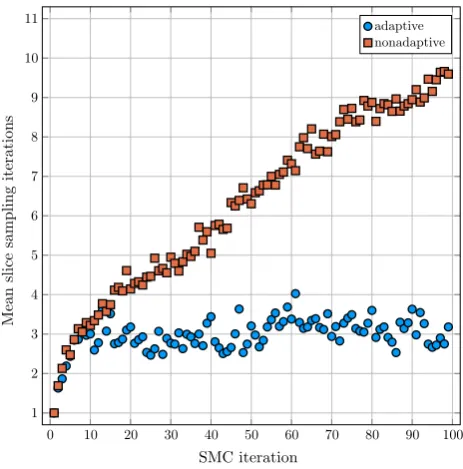
The only tuning choice required by Algorithm4 is the initial search widthw. A default choice isw = 1, but this means that the number of loops required will increase for small. To deal with this, we choosew=1 in the first SMC iteration and then selectwadaptively, as min(1,2¯z)wherez¯ is the maximum final value of|z|from all slice sampling calls in the previous SMC iteration. This choice generally shrinks wbased on the most recent value of¯z, while avoiding some unwanted behaviours. Firstly, it avoids forcingwto decrease at a fixed rate, so that eventually only very small steps would be attempted. Secondly, it avoidswgrowing above 1, which would make slice sampling expensive when local moves are required. The effect of our choice is investigated empirically later (see Fig.3).

3 High-dimensional ABC

This section presents our approach to inference in the ABC setting, using the algorithms reviewed in Sect.2. Section3.1 describes how the RE-SMC algorithms can estimate the ABC likelihood given values of θ and , and a latent variable structure. Such likelihood estimators can be used within sev-eral inference algorithms to produce approximate Bayesian inference. In this paper, we concentrate on PMMH. Sec-tion3.2presents the resulting method. Section3.3discusses the computational cost of the resultingRE-ABC algorithmin comparison with standard ABC, with particular note of the high-dimensional case.

Two versions of RE-ABC are possible, depending on whether likelihood estimates are produced using FIXED-RE-SMC or ADAPT-RE-FIXED-RE-SMC. We present both and compare them throughout the remainder of the paper. As will be

explained, in Sects. 3.2 and6.2, we conclude by arguing in favour of using FIXED-RE-SMC together with an initial run of ADAPT-RE-SMC to select thesequence.

3.1 Likelihood estimation

For now, supposeθand >0 are fixed. We aim to produce an unbiased estimate ofLABC(θ;), as defined in (2).

Suppose there exist latent variablesxsuch that the obser-vations can be written as a deterministic function y = y(θ,x). The idea is thatxandθsuffice to specify a complete realisation of the simulation process, even including details such as observation error, andy(θ,x)is a vector of partial observations. Neglectingθ, which is fixed for now,y(θ,x) will be written below as simplyy=y(x). See Sect.6.1for a discussion of properties ofy(θ,x)which help our approach work well.

We specify a densityπ(x|θ)(with respect to Lebesgue measure) for the latent variables. This is part of the specifi-cation of the model, but it can also be viewed as representing prior beliefs about the latent variables. Throughout the paper, we take π(x|θ) to be uniform on [0,1]m _{regardless of θ.}

Under this interpretation,xis a vector ofmindependent stan-dard uniform random variables which suffice to carry out the simulation process.

Now, we simply apply one of the RE-SMC algorithms usingΦ(x)=d(y(x),yobs). The small probability estimated

by these algorithms is

Pr(Φ(x)≤|θ)=

π(x|θ)1[d(y(x),yobs)≤t]dx

=

π(y|θ)1[d(y,yobs)≤t]dy,

which equals LABC(θ;)multiplied by the constant V().

Hence, using FIXED-RE-SMC we can obtain an estimate of LABC(θ;)which is unbiased, as required by PMMH. Using

ADAPT-RE-SMC produces a slightly biased estimate, and we comment on the effect of using this within PMMH in the next section.

3.2 Inference

Algorithm 5 shows the PMMH algorithm for our setting, which we refer to as RE-ABC. It can use either FIXED-RE-SMC or ADAPT-FIXED-RE-SMC when estimates of the ABC likelihood are required. We’ll use the prefixes FIXED and ADAPT to refer to the version of RE-ABC based on the corresponding RE-SMC algorithm.

Algorithm 5 Pseudo-marginal Metropolis–Hastings using RE-SMC (RE-ABC)

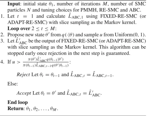
Input: initial stateθ1, number of iterations M, number of SMC particlesNand tuning choices for PMMH, RE-SMC and ABC. 1. Let t = 1 and calculate LˆABC,1 using FIXED-RE-SMC (or

ADAPT-RE-SMC) with slice sampling as the Markov kernel. Loop over2≤t≤M:

2. Propose new stateθ fromq(·|θ)and sampleufrom Uniform(0,1). 3. LetLˆ_ABCbe the output of FIXED-RE-SMC (or ADAPT-RE-SMC) with slice sampling as the Markov kernel. This algorithm can be stopped early once rejection in the next step is guaranteed. 4. Ifu> π(θ)LˆABCq(θt−1|θ)

π(θt−1)LˆABC,t−1q(θ|θt−1):

RejectLetθt=θt−1andLˆABC,t= ˆLABC,t−1. Else:

AcceptLetθt=θ andLˆABC,t= ˆLABC. End loop

Return:θ1, θ2, . . . , θM.

For FIXED-RE-ABC, the likelihood estimates are unbi-ased estimates ofLABC(θ;)up to proportionality.

There-fore, the probability of acceptance in step4corresponds to a target density proportional toπ(θ)LABC(θ;), i.e., the

stan-dard ABC posterior (1). ADAPT-RE-ABC involves biased likelihood estimates so does not sample from exactly this density. However, the bias introduced is small and may have little effect compared to the efficiency benefits of the variance reduction which ADAPT-RE-SMC provides (theoretical and practical aspects of MCMC algorithms that have this charac-ter are discussed inAlquier et al. 2016). We investigate this empirically in Sects.4and5and find no noticeable effect of bias. However, we find ADAPT-RE-SMC to sometimes be less computationally efficient in practice, and so we recom-mend using the FIXED-RE-SMC algorithm, together with a single run of ADAPT-RE-SMC to select asequence. Rea-sons for this are described shortly, and discussed in more detail in Sect.6, together with possibilities for improvement. To reduce computational costs RE-SMC can be terminated as soon as rejection is guaranteed. To implement this, after step 2 of RE-SMC check whether

tSMC

τ=1

ˆ

P_τ < uπ(θt−1)LˆABC,t−1q(θ|θt−1)

π(θ)q(θt−1|θ) ,

wheretSMC is the current value of thet variable within the

RE-SMC algorithm. If this is true, terminate the RE-SMC algorithm and reject the current proposal in the PMMH algo-rithm. The MCMC algorithm remains valid since the final RE-SMC likelihood estimate is guaranteed to be smaller than tSMC

τ=1 Pˆτ and therefore lead to rejection in PMMH.

Early termination prevents extremely long runs of RE-SMC forθvalues with low posterior densities. It is most efficient for FIXED-RE-SMC, where it is always possible to termi-nate in any iteration if the Pˆ_τ values are small enough. For ADAPT-RE-SMC, Pˆ_τ ≥ Nacc

N so there is a lower bound of

how many iterations are required before termination. This argument suggests ADAPT-RE-SMC is less computationally efficient and agrees with later empirical findings (see Fig.5). Earlier we commented that ADAPT-RE-SMC can fail to terminate in some situations. When ties in the distance are not possible, then this is usually not a problem within RE-ABC due to the early termination rule just outlined. However, care is still required the first time ADAPT-RE-SMC is run, and when it is used in pilot runs. Ties in the distance are potentially more problematic and are discussed further in Sect.6.3.

There are numerous tuning choices required in this PMMH algorithm. Most of these can be based on the output of a pilot analysis, for example an ABC analysis or a short initial run of PMMH. The estimated posterior meanμˆ can be used as an initial PMMH state. The estimated posterior varianceˆ can be used to tune the PMMH proposal density. Following the PMMH theory discussed in Sect.2.2, we sample proposal increments fromN

0,2_dim.562_(θ)2ˆ

(note that the early termi-nation rule avoids SMC calls having very long run times for someθ values, approximately meeting the assumptions of the PMMH tuning literature). The threshold sequence for FIXED-RE-SMC can be selected by running ADAPT-RE-SMC withθ = ˆμ. To select the number of particles, a few preliminary runs of FIXED-RE-SMC (or ADAPT-RE-SMC) can be performed with θ = ˆμ, aiming to produce a log-likelihood variance of roughly 1. This is at the more conserva-tive end of the range suggested by the theory reviewed earlier. A crucial tuning choice which remains is. As in other ABC methods, we suggest tuning this pragmatically based on the computational resources available. This can be done by running ADAPT-RE-SMC withθ= ˆμand=0 and stop-ping after a prespecified time, corresponding to how long is available for an iteration of PMMH. The value of t when

3.3 Cost

Here, we summarise results on the cost of ABC and RE-ABC in terms of time per samples produced (or effective sample size for PMMH algorithms), in the asymptotic case of small. Arguments supporting these results are given in “Appendix A”. Several assumptions are required, principally thatπ(y|θ)is a density with respect to Lebesgue measure— informally, the observations must be continuous. Weakening these assumptions is discussed in supplementary material. Note that the results are the same whether FIXED-RE-ABC and ADAPT-RE-ABC is used.

The time per sample is asymptotic to 1/V()for ABC and[logV()]2_{for RE-ABC (see (3) for definition ofV().)}

So, asymptotically, RE-ABC has a significantly lower cost to reach the same target density. To illustrate the effect of D=dim(y), we can consider the asymptotic case of large D(n.b. as shown in the supplementary material, when some observations are non-continuous thenDcan be replaced with the dimension of{y|d(y,yobs) < }for small.) Under the

Lebesgue assumption, (3) gives thatV()∝D. Hence, the time per sample is asymptotic to the following expressions, written in terms ofτ = 1/for interpretability: C1 = τD

for ABC andC2 = D2[logτ]2 = [logC1]2 for RE-ABC.

Hence, ABC has an exponential cost inD, while RE-ABC has only a quadratic cost. This makes high-dimensional infer-ence more tractable for RE-ABC but dimension reduction via summary statistics will remain useful in controlling the cost whenDis large.

These results assume the algorithms are run sequentially. The PMMH stage of RE-ABC is innately sequential, but particle updates can be run in parallel, providing a benefit from parallelisation. Compared to the most efficient ABC algorithms, this is an advantage over ABC-MCMC and seems roughly comparable to that of ABC-SMC algorithms.

4 Gaussian example

In this section, we compare ABC (Algorithm1) and RE-ABC (Algorithm5) on a simple Gaussian model. The model isYi ∼N(0, σ2)independently for 1≤i ≤25. We use the

priorσ ∼ Uniform(0,10). This is an interesting test case because dim(y)is large enough to cause difficulties for ABC methods but calculations are quick, and the results can be compared to those of likelihood-based methods.

4.1 Comparison of ABC and RE-ABC

We compared ABC and RE-ABC for observations drawn from the model usingσ =3. For each of=8,9, . . . ,30, we ran ABC untilN =500 simulations were accepted and calculated the root-mean-squared error and time per

accep-tance. Both FIXED-RE-ABC and ADAPT-RE-ABC were run for 2000 iterations with = 3,5,10,15,20,25. As described in Sect.3.2, pilot runs were used to tune the num-ber of particles, the Metropolis–Hastings proposal standard deviation and, where necessary, the threshold sequence. We chose the number of acceptances in all ADAPT-RE-ABC analyses to be half the number of particles. To avoid deal-ing with burn-in, we started the PMMH chains at σ = 3. For comparison, we also ran ABC-MCMC (Marjoram et al. 2003) and MCMC using the exact likelihood.

Figure1shows the results. The left panel illustrates that accuracy improves as the acceptance thresholdis reduced below roughly 15, and, as expected, all methods produce very similar results. In particular, the biased likelihood esti-mates in ADAPT-RE-ABC have a negligible effect overall. The right panel investigates the time taken per sample by ABC. For MCMC output, this is time divided by the effec-tive sample size (the IMSE estimate ofGeyer 1992.) Under ABC and ABC-MCMC, time per sample increases rapidly asis reduced. For both RE-ABC algorithms, the increase is slower, allowing smaller values ofto be investigated. Nei-ther RE-ABC algorithm is obviously more efficient than the other. This difference between ABC and RE-ABC is consis-tent with the asymptotics on computational cost described in Sect.3.3. However, for largevalues ABC and ABC-MCMC are cheaper. Overall, RE-ABC permits smallervalues to be investigated at a reasonable computational cost, producing more accurate approximations.

Figure2provides some further insight into the efficiency of the RE-ABC algorithms, by looking at the times taken for calls to the RE-SMC algorithms. These have similar distribu-tions for FIXED-RE-ABC and ADAPT-RE-ABC, indicating that there is little difference in their efficiency. One point of interest is that ADAPT-RE-SMC takes a minimum time of 0.095 seconds even when it stops early, while FIXED-RE-SMC sometimes stops early in a much shorter time. However, this happens too rarely to have much effect on overall effi-ciency.

4.2 Validity of assumptions

How-0 5 10 15 20 25 30 0.4

0.6 0_.8 1 1.2 1_.4 1_.6 1.8 2 2_.2

threshold

RMSE

0 2 4 6 8 10 12 14 16 18 20 22 24 26 28 30

10−6 10−5 10−4 10−3 10−2 10−1 100 101 102

threshold

time

/

E

SS

(s)

ABC ABC-MCMC ADAPT-RE-ABC FIXED-RE-ABC MCMC

Fig. 1 Simulation study comparing ABC, ABC-MCMC, FIXED-RE-ABC, ADAPT-RE-ABC and exact likelihood MCMC on IID Gaussian data

complete early

AD

APT−RE−ABC

FIXED−RE−ABC

0.0 0.1 0.2 0.0 0.1 0.2 0

100 200 300

0 100 200 300

time

count

Fig. 2 Histograms of times (in s) taken by calls to RE-SMC within FIXED-RE-ABC and ADAPT-RE-ABC analyses of IID Gaussian data. Both analyses used =5 and the same tuning details, chosen using a pilot run. Theleft columnis for those calls in which RE-SMC was completed, while therightshows those where it was terminated early

ever, adaptive tuning did increase the log-likelihood variance slightly so there is a small trade-off in its use.

Secondly, we investigated the distribution of likelihood estimates produced by FIXED-RE-SMC given a particu-larθ value. Recall that the theoretical literature on PMMH

0 10 20 30 40 50 60 70 80 90 100

1 2 3 4 5 6 7 8 9 10 11

SMC iteration

Mean

slice

sampling

iterations

adaptive nonadaptive

Fig. 3 Number of slice sampling iterations required under adaptive and non-adaptive rules for selecting the tuning parameterwwithin a run of FIXED-RE-SMC on IID Gaussian data

−2.5 −2 −1.5 −1 −0.5 0 0.5 1 1.5 2 2.5 3

−90

−85

−80

−75

−70

−65

−60

Sample quantile

Theoretical

quan

tile

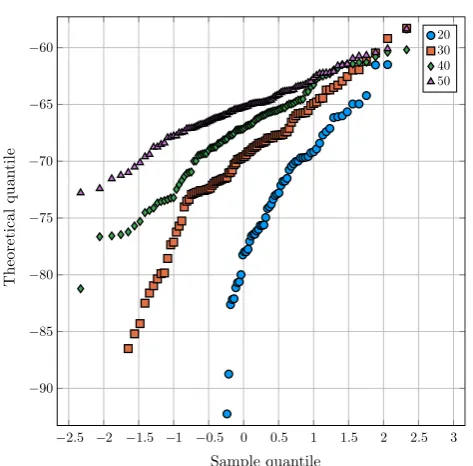
20 30 40 50

Fig. 4 Normal quantile-quantile plots of log-likelihood estimates for an FIXED-RE-SMC example under various numbers of particles. Omit-ted points correspond to likelihood estimates of zero

points are omitted from the plot. In conclusion, the normal-ity assumption seems reasonable if a sufficient number of particles are used.

5 Epidemic application

Infectious disease data are often modelled using compart-ment modelswhere members of a population pass through several stages. We will consider a model with susceptible, infectious and removed stages – the so-called SIR model (Andersson and Britton 2000). A susceptible individual has not yet been infected with the disease but is vulnerable. An infectious individual has been infected and may spread the disease to others. A removed individual can no longer spread the disease. Depending on the disease this may be due to immunity following recovery, or death.

We will use a stochastic version of this model based on a continuous time stochastic process{S(t),I(t) : t ≥ 0} for numbers susceptible and infectious at timet. The total population size is fixed atnso the number removed at time t can be derived as R(t) = n −S(t)− I(t). The initial conditions are(S(0),I(0)) = (n −1,1). Two jump tran-sitions are possible: infection(i,j) → (i −1,j+1)and removal (i,j) → (i,j −1). The simplest version of the model is Markovian and is defined by the instantaneous haz-ard functions of the two transitions, which areλ_nS(t)I(t)for infection andγI(t)for removal. The unknown parameters areλ, controlling infection rates andγ, the removal rate. A goal of inference is often to learn about the basic reproduction

number R0 =λ/γ. This is the expected number of further

infections caused by an initial infected individual in a large susceptible population. When R0<1, most epidemics will

infect an insignificant proportion of a large population. Many variations on the Markovian SIR model are possible, some of which are outlined below.

Likelihood-based inference is straightforward for fully observed data from an SIR model. However, in practice only partial and possibly noisy observations of removal times are available, producing an intractable likelihood. For many models near-exact inference is possible by MCMC methods (summarised by McKinley et al. 2014), but small changes to the details require new and model-specific algorithms. Approximate inference can be performed by ABC (sum-marised byKypraios et al. 2016), which is more adaptable but does not scale well to high-dimensional data. Here, we illustrate how RE-ABC can, without modification, perform inference for several variations on the SIR model, and do so more efficiently than standard ABC methods. As we concen-trate on a classic and well-studied dataset, our analysis does not provide any novel subject-area insights.

Section5.1describes a method of simulating from SIR models. Section5.2discusses the distance function we use to implement RE-ABC. Data analysis is performed in Sect.5.3.

5.1 Sellke construction

The Sellke construction (Sellke 1983) for an SIR model provides an appealing way to simulate epidemic models. It introduces latentinfectious periods gi ∼ Finfandpressure

thresholds pi ∼Fpressfor 1≤i ≤n, all independent. For the

Markovian SIR model,FinfisE x p(γ )andFpressisE x p(1),

but other choices are possible and may be more biologically plausible. We condition ong1=0 so that the first infection

occurs at time 0. Algorithm6shows how these variables and the parameterλ are converted to simulated removal times. To use slice sampling, we require the latent variables to be uniformly distributed a priori. Therefore, we use quantiles of thegis and pis as the latent variables.

The cost of Algorithm 6 is O(nlogn), where n is the population size. This is because the main loop runs at most 2n−1 times and involves finding the minimum of a set of up ton−1 removal times, which requiresO(logn)steps (this is the case if the set is stored as an ordered vector. The cost of adding a new item isO(logn)).

jump will typically have a large and unpredictable effect on all the subsequent jumps. For more discussion on desirable properties ofy(θ,x), see Sect.6.

Note that when Fpress is E x p(1) then R0 = λE(Finf)

(Andersson and Britton 2000). However, to our knowledge the definition ofR0has not been extended to cover general

Fpress.

Algorithm 6Sellke construction epidemic simulator Input: population sizen, scaled infection rate parameterβ=λ/n, infectious periodsg1, . . . ,gnand pressure thresholdsp2, . . . ,pn.

1. Setr1→g1(assumes individual 1 has infection time 0). 2. Setri→ ∞fori>2.

3. SetI →1 (current number infected),t→0 (current time),p→0 (current pressure).

4. WhileI>0:

5. Findpa=min{pi|pi>p}. If this set is empty usepn+1= ∞. 6. Findrb=min{ri|ri>t}.

7. Setp →p+βI(rb−t)(pressure at timerbifIdoes not change)

8. Ifpa<p:

(a) SetI→I+1,t→t+pa−p

βI ,ra→t+ga,p→ pa.

9. Else:

(a) SetI→I−1,t→rb,p→p.

10. End while

Output: Removal timesr1,r2, . . . ,rn. Infinite removal time

repre-sents an individual who is never infected.

5.2 Distance function

Recall that the data are the inter-removal times, or equiv-alently the times since the first removal. For a simulated dataset, let r₍1) ≤ r(2) ≤ . . . ≤ r(ν) denote the ordered

removal times of a dataset withνremovals. The times since first removal are thens₍i₎=r₍i₎−r₍1₎for 1≤i ≤ν. Similar

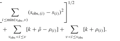
notation, with the addition of a subscriptobswill be used for the observed dataset. We define the distance between a simulated and observed dataset as:

⎡

⎣

i_≤min_(νobs,ν)

(sobs,(i)−s(i))2 ⎤ ⎦

1/2

+

νobs<i≤ν

[k+ ¯ρ−ρ₍i)] +

ν<i≤νobs

[k+ρ₍i)].

(5)

Here,kis a tuning parameter penalising mismatches between νandνobs. We takek=1000. Theρ₍i₎terms are the sorted

simulated pressure thresholds andρ¯ is the total simulated pressure (which equalsβtimes the sum of the infectious peri-ods for removed individuals). They are included to encourage these pressures to increase or decreasing appropriately to

matchνandνobs. Without the pressure terms RE-SMC

per-formed poorly due to the discrete nature ofν. See Sect.6.3 for further discussion.

5.3 Analysis of Abakaliki data

The Abakaliki dataset contains times between removals from a smallpox epidemic in which 30 individuals were infected from a closed population of 120. It has been studied by many authors under many variations to the basic SIR model. We study three models. The first model uses a Gamma(k, γ ) infectious period (similar toNeal and Roberts 2005). The second assumes pressure thresholds are distributed by a Weibull(k,1)distribution (as inStreftaris and Gibson 2012.) The third is the Markovian SIR model, but with removal times only recorded within 5 day bins. This is realised by alter-ing thesobs,(i)−s(i)term (difference between simulated and

observed day of removal) in (5) to f(sobs,(i))−f(s(i))where

f(s)=5s/5, the greatest multiple of 5 less than or equal to s. In each model, there are two or three unknown parameters: λ, controlling infection rates;γ, infectious period scale;k, a shape parameter. These are all assigned independent expo-nential prior distributions with rate 0.1, representing weakly informative prior beliefs that these parameters are less likely to be large.

We chose the acceptance threshold to be = 15 on the pragmatic grounds that this produced run times of no more than 6 hours on a desktop PC. Tuning was performed using pilot runs as described in Sect. 3.2. Of particular note is the number of particles required: 300 (Gamma infectious period), 200 (Weibull pressure thresholds) and 400 (binned removal times). First we present results for FIXED-RE-ABC, with discussion on ADAPT-RE-ABC to follow shortly. Table1summarises the approximate posterior results. As the parameters differ between models, we don’t present param-eter estimates. Instead, we give several quantities of interest for each: the R0 estimate (where defined) and the means

and standard deviations of (a) the pressure thresholds and (b) the infectious period. Most quantities are similar to each other and previous analyses (seeMcKinley et al. 2014for a summary of many of these) despite the different modelling assumptions. A noticeable difference is that the infectious period is less variable in the model where it follows a Gamma distribution.

Table 1 Approximate posterior estimates of basic reproduction numberR0and the means and standard deviations of pressure thresholds and infectious periods for the Abakaliki data under three models computed using FIXED-RE-ABC

Model R0 Pressure thresholds Infectious period

Mean SD Mean SD

5 day bins 1.16 (0.30) 0.11 (0.03) 0.11 (0.03) 11.1 (3.0) 11.1 (3.0)

Gamma infectious period 1.18 (0.24) 0.09 (0.03) 0.09 (0.03) 13.6 (3.8) 6.8 (2.2)

Weibull pressure thresholds – 0.10 (0.04) 0.11 (0.03) 12.4 (3.3) 12.4 (3.3)

The table contains Monte Carlo estimates along with standard deviations in brackets. TheR0value is not given for the Weibull pressure threshold model as no definition is available for this model

differing number of parameters in the models. So we con-clude qualitatively that are no clear differences in fit between the models.

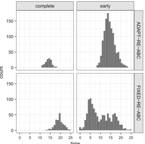
ADAPT-RE-ABC was also tried and returned parameter inference results extremely similar to those for FIXED-RE-ABC – see Table 1 in the supplementary material. This shows that, as in Sect.4, the bias in its likelihood estimates has a neg-ligible effect on the final results. However, for some analyses the run times were longer. For example, the Gamma infec-tious period model took 263 minutes for FIXED-RE-ABC and 323 minutes for ADAPT-RE-ABC. Figure5investigates this in more detail. It shows that the run time difference is because most calls to RE-SMC terminate early, and these are generally quicker under FIXED-RE-SMC. It is also interest-ing that ADAPT-RE-SMC is typically faster for completed

complete early

AD

APT−RE−ABC

FIXED−RE−ABC

0 5 10 15 20 25 0 5 10 15 20 25

0 50 100 150

0 50 100 150

time

count

Fig. 5 Histograms of times (in s) taken by calls to RE-SMC within FIXED-RE-ABC and ADAPT-RE-ABC analyses of Abakaliki data. Both analyses used=15 and the same tuning details, chosen using a pilot run. Theleft columnis for those calls in which RE-SMC was completed, while therightshows those where it was terminated early

RE-SMC calls. These findings are discussed in the next sec-tion.

We also ran ABC-MCMC for comparison, using the same MCMC andtuning choices as for RE-ABC. For run times of comparable length to RE-ABC, ABC-MCMC produced too few acceptances to calculate effective sample sizes accu-rately. Instead, we consider the time per acceptance. For ABC-MCMC this was at least 12 minutes for all models. For RE-ABC, this value was always less than 2 minutes.

6 Discussion

We have presented a method for approximate inference under an intractable likelihood when simulation of data is possible. It uses the same posterior approximation as ABC, (1), which is controlled by a tuning parameter. The advantage of our method is that smaller values ofcan be achieved for the same computational cost, resulting in more accurate infer-ence. We have shown this is the case through asymptotics (Sect.3.3) and empirically (Sects.4,5.) This increased accu-racy allows higher-dimensional data or summary statistics to be analysed in practice.

6.1 Latent variable considerations

Our method represents the model of interest with latent vari-ables x and uses SMC and slice sampling to search for promising x values. For this search strategy to work well, it seems necessary that:

– Evaluatingy(θ,x)is reasonably cheap.

– Sets of the form {x|d(yobs,y(θ,x)) ≤ }are easy to

explore using slice sampling. This would be difficult for sets made up of many disconnected components, or which are lower dimensional manifolds. Smoothness of yto changes inxwill help meet this condition.

the slice sampling algorithm (see Section 4.2 ofMurray and Graham 2016).

6.2 Adaptive and non-adaptive algorithms

The RE-ABC algorithm can use RE-SMC with a fixed sequence (FIXED-RE-SMC) or one that is chosen adaptively (ADAPT-RE-SMC). FIXED-RE-SMC provides unbiased estimates of the ABC likelihood, as required by the PMMH algorithm, while ADAPT-RE-SMC has a small bias. In prac-tice, we observe very little difference in the posterior results between the two algorithms, suggesting that this bias has a negligible effect in practice. We also note that, if desired, a bias correction approach fromCérou et al.(2012) could be applied.

Nonetheless, we recommend using the FIXED-RE-SMC algorithm within RE-ABC (together with a pilot run of ADAPT-RE-SMC to choose thesequence.) The main rea-son is that it is faster to run in practice, as found in Sect.5. Figure5 shows that this is because FIXED-RE-SMC can terminate more quickly for poor proposedθvalues. Interest-ingly, in the iterations where early termination is not required ADAPT-RE-SMC is slightly quicker. We speculate that this is because it often finds a shortersequence. Furthermore, the theory of Cérou et al. (2012) suggests that ADAPT-RE-SMC produces less variable ABC likelihood estimates, which would improve PMMH efficiency. Therefore, there may be some scope for a more efficient RE-SMC algorithm which combines the best features of the adaptive and non-adaptive approaches.

6.3 Possible extensions

More efficient sequence adaptation ADAPT-RE-ABC adapts thesequence for eachθvalue separately. One alter-native is to instead update the sequence based on information from SMC runs at previousθ values used by PMMH. This could be done using stochastic approximation (see, e.g., Andrieu and Thoms 2008;Garthwaite et al. 2016), with the aim of making the Pˆt values in Algorithm 2 as similar as

possible—which minimises asymptotic variance of the like-lihood estimates, as discussed in Sect.2.3. The result would be an adaptive MCMC algorithm, and it may be theoretically challenging to prove it has desirable convergence properties (Andrieu and Thoms 2008).

Joint exploration of (θ,x)Manyθvalues proposed by RE-ABC are rejected after calculating an expensive likelihood estimate. An appealing alternative is to update the parame-tersθconditional on sampledxvalues, for example through a Gibbs sampler with state(θ,x). Unfortunately in exploratory analyses of such methods, we found theθupdates generally did not mix well. The reason is thatxis much more

infor-mative forθthan the observationsyobs. This results in small θmoves compared to the posterior’s scale.

Alternatively, one could consider nesting an SMC algo-rithm to explorexwithin one to exploreθ, followingChopin et al. (2013) and Crisan and Miguez (2016). Exploring θ could proceed by reducing at each iteration. This might avoid the time penalty of ADAPT-RE-SMC when used in PMMH, discussed in Sect.6.2.

Discrete data RE-SMC can struggle if there is a discrete data variablex∗. It can be hard for SMC to move from accepting a set of latent variablesAto anotherA in which the range of possiblex∗values is smaller, because Pr(x ∈ A|x ∈ A, θ) may be very small. The issue is particularly obvious for ADAPT-RE-SMC as thesequence may fail to move below some threshold for a large number of iterations. For FIXED-RE-SMC, it would instead result in high-variance likelihood estimates. In Sect.5.2, this problem occurs forν, the number of removals. There we adopt an application-specific solution by introducing continuous latent variables (pressure thresh-olds) into the distance function (5). It would be useful to investigate more general solutions from the rare event lit-erature (e.g., Walter 2015). Despite these potential issues, RE-ABC can perform well with discrete data in practice, for example in the binned data model of Sect.5.3.

Non-uniform ABC kernels In this paper, the ABC likelihood (2) is a convolution of the exact likelihood and a uniform kernel (4). Alternative kernel functions have also been used in ABC (e.g.,Wilkinson 2013) such as a Gaussian:k(y;)∝ exp[−₂12d(y,yobs)]. RE-ABC could easily be adapted to

make use of these, but it is not clear what effect it would have on our asymptotic results.

Estimating log-likelihood gradients Where log-likelihood gradients can be estimated they allow more efficient infer-ence schemes based on stochastic gradient descent (Poyiadjis et al. 2011) or MCMC (Dahlin et al. 2015). Estimating such gradients from SMC algorithms is possible using the Fisher identity (Poyiadjis et al. 2011). However, the calculation would involve evaluating∇_θy(θ,x), which may be demand-ing for complicated yfunctions. Moreno et al.(2016) use automatic differentiation to evaluate this for some models. Alternatively,Andrieu et al.(2012) propose using infinites-imal perturbation analysis methods. It would be interesting to use either approach with RE-ABC.

use our likelihood estimate in algorithms which directly out-put model evidence estimates, such as importance sampling or population Monte Carlo (Cappé et al. 2004).

Acknowledgements We thank Chris Sherlock for suggesting the use of slice sampling and Andrew Golightly for helpful discussions. Open Access This article is distributed under the terms of the Creative Commons Attribution 4.0 International License (http://creativecomm ons.org/licenses/by/4.0/), which permits unrestricted use, distribution, and reproduction in any medium, provided you give appropriate credit to the original author(s) and the source, provide a link to the Creative Commons license, and indicate if changes were made.

Appendix A: Computational cost

This appendix justifies the computational costs of ABC and RE-ABC stated in Sect.3.3. The argument for ABC is rig-orous, while that for RE-ABC is more heuristic. Note that throughout this appendix there is no need to distinguish between FIXED-RE-ABC and ADAPT-RE-ABC.

The results are for the asymptotic regime of smalland hold for almost allyobs. We make several assumptions:

A1 The densityπ(y|θ)is with respect to Lebesgue measure dyof dimensionD.

A2 The distance function is Euclidean distance.

A3 Running slice sampling once requires O(1) function evaluations.

A4 RE-SMC usesO(−log Pr(d(y,yobs)≤|θ))iterations.

A5 The time required to evaluatey(θ,x)is bounded above and below by nonzero constants which do not depend onθorx.

Also, we will usually focus on the case whereDis asymp-totically large.

Informally, A1 requires that all components ofyhave con-tinuous distributions. Under A2 a key mathematical result below, (6), follows easily. Also, a consequence of A2 which we will use is that, from (3),V()∝−D_{. A3 states that the}

cost of slice sampling does not increase asshrinks. This is plausible due to our adaptive choice ofw(see Sect.2.4) and was empirically verified above (see Fig.3.) It follows that running RE-SMC requiresO(N T)function evaluations: the number is asymptotic to the number of particles multi-plied by the number of SMC iterations. A4 states that the number of iterations used by RE-SMC is asymptotically proportional to the log of the rare probability being esti-mated. This follows from a result of Cérou et al.(2012), reviewed in Sect. 2.3, that when the RE-SMC algorithm is tuned optimally Pr(Ak+1|θ,x ∈ Ak)is constant, sayα,

whereAkdenotes the eventd(y(θ,x),yobs)≤k. Therefore,

Pr(d(y,yobs)≤|θ)=αT, and taking logs gives A4. So the

assumption is that RE-SMC is tuned to perform similarly to optimal tuning. Assumption A5 states that performing a simulation has a minimum and maximum time requirement regardless of the inputs, which is usually reasonable. This ensures that computation time is asymptotic to the number of simulations performed.

Many of these assumptions can be weakened. This is dis-cussed in the supplementary material, especially for the case of the epidemic model of Sect.5.

A.1 ABC

Consider the probability of a simulation being accepted given θ:

Pr(d(y,yobs)≤|θ)=

π(y|θ)1(d(y,yobs)≤)dy.

By the Lebesgue differentiation theorem (see Stein and Shakarchi 2009for example) for almost allyobs:

lim

→0V()

−1

π(y|θ)1(d(y,yobs)≤)dy=π(yobs|θ),

(6)

Hence for small:

Pr(d(y,yobs)≤|θ)∼V(), (7)

where∼represents an asymptotic relation (note that while π(yobs|θ)does not affect this asymptotic relationship, the

acceptance probability will decrease for small π(yobs|θ),

i.e., for poorθchoices).

By assumption A5 the time per accepted sample is asymp-totic to the number of simulations per accepted sample. Using (7), the latter is asymptotic to 1/V(). In the case of large Dassumption A2 gives that this is O(τD), where τ =1/. For ABC versions of MCMC and SMC, time per accepted sample (or effective sample) is also bounded below by min_θPr(d(y,yobs)≤|θ)−1, so the same result applies.

A.2 RE-ABC

number of simulations required by an iteration of RE-ABC isO(T2). Using A4 and (7) givesT =O(−logV()).

So the number of simulations required per iteration of RE-ABC isO([logV()]2). In the case of largeDusing A2 gives that this isO(D2[logτ]2). As in the previous section, assumption A5 implies these expressions also give the time per sample of RE-ABC. They are also valid for the more relevant quantity of time per effective sample since effective sample size is proportional to the actual sample size.

References

Alquier, P., Friel, N., Everitt, R., Boland, A.: Noisy Monte Carlo: con-vergence of Markov chains with approximate transition kernels. Stat. Comput.26(1), 29–47 (2016)

Andersson, H., Britton, T.: Stochastic Epidemic Models and Their Sta-tistical Analysis. Springer, Berlin (2000)

Andrieu, C., Doucet, A., Lee, A.: Contribution to the discussion of Fearnhead and Prangle (2012). J. R. Stat. Soc. B74, 451–452 (2012)

Andrieu, C., Roberts, G.O.: The pseudo-marginal approach for efficient Monte Carlo computations. Ann. Stat.39, 697–725 (2009) Andrieu, C., Thoms, J.: A tutorial on adaptive MCMC. Stat. Comput.

18(4), 343–373 (2008)

Barber, S., Voss, J., Webster, M.: The rate of convergence for approxi-mate Bayesian computation. Electron. J. Stat.9, 80–105 (2015) Beaumont, M.A., Zhang, W., Balding, D.J.: Approximate Bayesian

computation in population genetics. Genetics 162, 2025–2035 (2002)

Biau, G., Cérou, F., Guyader, A.: New insights into approximate Bayesian computation. Annales de l’Institut Henri Poincaré (B) Probabilités et Statistiques51(1), 376–403 (2015)

Blum, M.G.B.: Approximate Bayesian computation: a nonparametric perspective. J. Am. Stat. Assoc.105(491), 1178–1187 (2010) Blum, M.G.B., Nunes, M.A., Prangle, D., Sisson, S.A.: A comparative

review of dimension reduction methods in approximate Bayesian computation. Stat. Sci.28, 189–208 (2013)

Cappé, O., Guillin, A., Marin, J.-M., Robert, C.P.: Population Monte Carlo. J. Comput. Gr. Stat.13(4), 907–929 (2004)

Cérou, F., Del Moral, P., Furon, T., Guyader, A.: Sequential Monte Carlo for rare event estimation. Stat. Comput.22(3), 795–808 (2012) Chiachio, M., Beck, J.L., Chiachio, J., Rus, G.: Approximate Bayesian

computation by subset simulation. SIAM J. Sci. Comput.36(3), A1339–A1358 (2014)

Chkrebtii, O.A., Cameron, E.K., Campbell, D.A., Bayne, E.M.: Trans-dimensional approximate Bayesian computation for inference on invasive species models with latent variables of unknown dimen-sion. Comput. Stat. Data Anal.86, 97–110 (2015)

Chopin, N., Jacob, P.E., Papaspiliopoulos, O.: SMC2_{: an efficient} algo-rithm for sequential analysis of state space models. J. R. Stat. Soc. Ser. B (Stat. Methodol.)75(3), 397–426 (2013)

Crisan, D., Miguez, J.: Nested particle filters for online param-eter estimation in discrete-time state-space Markov models. arXiv:1308.1883(2016)

Dahlin, J., Lindsten, F., Schön, T.B.: Particle Metropolis–Hastings using gradient and Hessian information. Stat. Comput. 25(1), 81–92 (2015)

Del Moral, P., Doucet, A., Jasra, A.: An adaptive sequential Monte Carlo method for approximate Bayesian computation. Stat. Com-put.22(5), 1009–1020 (2012)

Doucet, A., Pitt, M.K., Deligiannidis, G., Kohn, R.: Efficient imple-mentation of Markov chain Monte Carlo when using an unbiased likelihood estimator. Biometrika102(2), 295–313 (2015) Fearnhead, P., Prangle, D.: Constructing summary statistics for

approx-imate Bayesian computation: semi-automatic ABC. J. R. Stat. Soc. B74, 419–474 (2012)

Forneron, J.-J., Ng, S.: A likelihood-free reverse sampler of the posterior distribution. In: GonzÁlez-Rivera, G., Hill, R. C., Lee, T.-H. (eds.) Essays in Honor of Aman Ullah, pp. 389–415. Emerald Group Publishing Limited (2016)

François, O., Laval, G.: Deviance information criteria for model selec-tion in approximate Bayesian computaselec-tion. Stat. Appl. Genet. Mol. Biol.10(1) (2011). doi:10.2202/1544-6115.1678

Garthwaite, P.H., Fan, Y., Sisson, S.A.: Adaptive optimal scaling of Metropolis–Hastings algorithms using the Robbins–Monro pro-cess. Commun. Stat. Theory Methods45(17), 5098–5111 (2016) Geyer, C.J.: Practical Markov chain Monte Carlo. Stat. Sci.7, 473–483

(1992)

Graham, M.M., Storkey, A.: Asymptotically exact conditional infer-ence in deep generative models and differentiable simulators. arXiv:1605.07826(2016)

Jasra, A.: Approximate Bayesian computation for a class of time series models. Int. Stat. Rev.83, 405–435 (2015)

Kypraios, T., Neal, P., Prangle, D.: A tutorial introduction to Bayesian inference for stochastic epidemic models using Approximate Bayesian Computation. Math. Biosci.287, 42–53 (2016) L’Ecuyer, P., Demers, V., Tuffin, B.: Rare events, splitting, and

quasi-Monte Carlo. ACM Trans. Model. Comput. Simul. (TOMACS) 17(2), 9 (2007)

Li, J., Nott, D.J., Fan, Y., Sisson, S.A.: Extending approximate Bayesian computation methods to high dimensions via a Gaussian copula model. Comput. Stat. Data Anal.106, 77–89 (2017)

Marin, J.-M., Pudlo, P., Robert, C.P., Ryder, R.J.: Approximate Bayesian computational methods. Stat. Comput.22(6), 1167–1180 (2012) Marjoram, P., Molitor, J., Plagnol, V., Tavaré, S.: Markov chain Monte

Carlo without likelihoods. Proc. Natl. Acad. Sci.100(26), 15324– 15328 (2003)

McKinley, T.J., Ross, J.V., Deardon, R., Cook, A.R.: Simulation-based Bayesian inference for epidemic models. Comput. Stat. Data Anal. 71, 434–447 (2014)

Meeds, T., Welling, M.: Optimization Monte Carlo: efficient and embarrassingly parallel likelihood-free inference. In: Cortes, C., Lawrence, N.D., Lee, D.D., Sugiyama, M., Garnett, R. (eds.) Advances in Neural Information Processing Systems, pp. 2071– 2079. Curran Associates, Inc. (2015)

Moreno, A., Adel, T., Meeds, E., Rehg, J.M., Welling, M.: Automatic variational ABC.arXiv:1606.08549(2016)

Murray, I., Graham, M.M.: Pseudo-marginal slice sampling. J. Mach. Learn. Res.51, 911–919 (2016)

Neal, P.: Efficient likelihood-free Bayesian computation for household epidemics. Stat. Comput.22(6), 1239–1256 (2012)

Neal, P., Roberts, G.: A case study in non-centering for data augmenta-tion: stochastic epidemics. Stat. Comput.15(4), 315–327 (2005) Nott, D.J., Fan, Y., Marshall, L., Sisson, S.A.: Approximate Bayesian

computation and Bayes linear analysis: toward high-dimensional ABC. J. Comput. Gr. Stat.23(1), 65–86 (2014)

Nott, D.J., Ong, V.M.-H., Fan, Y., Sisson, S.A.: High-dimensional ABC. In: Scott, A., Sisson, Y.E., Beaumont, M. (eds.) Handbook of Approximate Bayesian Computation (Forthcoming). Chapman and Hall/CRC Press, Boca Raton (2017)

Pitt, M.K., Silva, R.D.S., Giordani, P., Kohn, R.: On some properties of Markov chain Monte Carlo simulation methods based on the particle filter. J. Econ.171(2), 134–151 (2012)