Multiagent Bayesian Forecasting of Time Series with Graphical Models

(1)

Multiagent Bayesian Forecasting of Time Series with Graphical Models

Yang Xiang

1

_{, James Smith}

2

_{and Jeff Kroes}

1

1_{University of Guelph, Canada} 2_{University of Warwick, UK}

Abstract

Time series are found widely in engineering and science. We study multiagent forecasting in time series, drawing from lit-erature on time series, graphical models, and multiagent sys-tems. Knowledge representation of our agents is based on dynamic multiply sectioned Bayesian networks (DMSBNs), a class of cooperative multiagent graphical models. We pro-pose a method through which agents can perform one-step forecast with exact probabilistic inference. Superior perfor-mance of our agents over agents based on dynamic Bayesian networks (DBNs) are demonstrated through experiment.

Introduction

Time series (Brockwell & Davis 1991) are found widely in engineering, science and economics, and allow useful in-ferences such as forecasting. Time series are traditionally studied under the single agent paradigm, but research under the multiagent paradigm has been seen in recent years, e.g., (Raudys & Zliobaite 2006) and (Kiekintveld et al. 2007).

Graphical models (Pearl 1988; Lauritzen 1996) have be-come an important tool for analyzing multivariate data. There is now a large literature on time series models which can be depicted by graphs. Some of the earliest models proposed are DBNs (Dean & Kanazawa 1989; Kjaerulff 1992). These graphs code a variety of conditional indepen-dence statements both with variables with the same time index and across time. One of the most successful of these is based on the class of vector autoregressive (VAR) models (Brockwell & Davis 1991) led by developments such as (Dahlhaus & Eichler 2003). A second approach adopted by (West & Harrison 1996; Koller & Lerner 2001; Pournara & Wernisch 2004; Queen & Smith 1993) develop state space analogues of these processes. Because of their simplicity and convenient closure properties, this paper fo-cuses on multiagent forecasting models of the first kind.

Under the multiagent paradigm, multiply sectioned Bayesian networks (MBSNs) (Xiang 2002) are proposed as cooperative multiagent graphical models. They are first ap-plied to static domains and have been extended to dynamic domains (An, Xiang, & Cercone 2008).

This paper proposes a technique for cooperative multia-gent forecasting with time series based on DMSBNs. For Copyright c2009, Association for the Advancement of Artificial Intelligence (www.aaai.org). All rights reserved.

these stochastic graphical models, their time series across (temporal) interface variables share the type of conditional independence structure of VAR models without linearity as-sumptions. Unlike (Raudys & Zliobaite 2006) where agents are “competing among themselves” for better financial pre-diction, agents based on DMSBNs are cooperative.

Background

Dynamic Bayesian network

A DBN (Dean & Kanazawa 1989; Kjaerulff 1992) models a dynamic domain over a finite time period. Our formulation follows that of (Xiang 1998).

Definition 1 A DBN of horizon k is a quadruplet G = (Sk_i₌₀Vi,Sk_i₌₀Gi,Sk_i₌₁Fi,Sk_i₌₀Pi). Vi is a set of

vari-ables for time intervali. Giis a DAG whose nodes are

la-beled by elements ofVi.Fiis a set of arcs each directed from

a node in Gi−1to a node inGi. Each nodev ∈ S k i=0Vi

is conditionally independent of its non-descendants given its parents π(v). Pi is a set of probability distributions

Pi={P(v|π(v))|v∈Vi}.

Gmodels a dynamic domain overk+ 1intervals, each of which is referred to as intervalior timei. Virepresents the

state of the domain at intervaliandGimodels the uncertain

dependency among elements ofVi. Fiis a set of temporal

arcs representing how the domain evolves over time. Definition 2 In a DBN G of horizon k, subset F Ii =

{x|∃(x, y) ∈ Fi+1}is the forward interface ofVi (0 ≤

i < k). SubsetBIi ={z|∃(x, y)∈Fi, z∈f mly(y)∩Vi}

is the backward interface of Vi (0 < i ≤ k). Denote

Gi = (Vi, Ei), where Ei is the set of arcs, and Di =

(Vi∪F Ii−1, Ei∪Fi). The pair Si = (Di, Pi)is a slice

of the DBN andDiis the structure ofSi.

2 e a b d e f c a b d f c a b d f e a b d e f 1 1 1 1 1 0 0 0 0 0 c0 c1 2 2 2 2 2 K K K K K K ... ... ... D1 D2 DK D0 Figure 1: An example DBN.

The joint probability distribution (jpd) of the domain over k+ 1intervals is the product of distributions in all slices.

(2)

Fig. 1 shows a DBN whereV1 ={a1, b1, c1, d1, e1, f1}, E1 = {(a1, b1),(b1, d1),(c1, e1),(d1, e1),(e1, f1)}, F1 = {(a0, b1),(f0, f1)}, F I1 = {a1, f1}, and BI1 = {a1, b1, e1, f1}. Note that subscripts are used to index tem-poral distribution of variables and dependency structures.

Multiply Sectioned Bayesian Networks

An MSBN models a domain, typically spatially distributed among a set of agents. The domain dependency is captured by a set of (overlapping) graphs, defined below and illus-trated in Fig. 2.

Definition 3 LetGi _{= (}_Vi_{, E}i_{) (}_i _{= 0}_,₁₎_{be two graphs.}

G0andG1are graph-consistent if subgraphs ofG0andG1

spanned byV0_∩_V1 _{(keeping nodes in}_V0_∩_V1 _{and arcs}

among them only) are identical. Given two graph-consistent graphsGi _{= (}_Vi_{, E}i_{) (}_i _{= 0}_,₁₎_{, the graph}_G _{= (}_V0_∪ V1, E0∪E1)is the union ofG0andG1, denoted byG= G0∪G1. Given a graphG= (V, E), a decomposition ofV

intoV0_and_V1_{such that}_V0_∪_V1₌_V _and_V0_∩_V1₆₌_∅_,

and subgraphsGi₍_i_{= 0}_,₁₎_of_G_{spanned by}_Vi_,_G_{is said}

to be sectioned intoG0_and_G1_.

section union b a d c e b a d c c d e

Figure 2: Illustration of graph union and section. To ensure exact probabilistic inference, distributed graph-ical models need to satisfy the following conditions. Def. 4 specifies how domain variables are distributed.

Definition 4 Let G = (V, E) be a connected graph sec-tioned into subgraphs{Gi _{= (}_Vi_{, E}i₎_}_{. Let the subgraphs}

be organized into an undirected tree Ψwhere each node is uniquely labeled by aGi_{and each link between}_Gk_and_Gm

is labeled by the non-empty interfaceVk ∩Vm such that for eachGi_and_Gj_in_Ψ_{and each}_Gx_{on the path between}

GiandGj,Vi∩Vj ⊂Vx. ThenΨis a hypertree overG. EachGi_{is a hypernode and each interface is a hyperlink.}

A pair of hypernodes connected by a hyperlink is said to be

Figure 3: A trivial MSBN with hypertreeG1−G0−G2. Fig. 3 shows three subgraphs which section a graphG(not shown). A corresponding hypertree has the topologyG1−

G0−G2. Def. 5 specifies what variables agent interfaces contain. This condition ensures conditional independence given the interface.

Definition 5 LetGbe a directed graph sectioned into sub-graphs{Gi}such that a hypertree overGexists. A node

x(whose parent set in G, possibly empty, is denotedπ(x)) contained in more than one subgraph is a d-sepnode if there exists at least one subgraph that containsπ(x). An interface

I is a d-sepset if everyx∈I is a d-sepnode.

For the above hypertree related to Fig. 3, it has two iden-tical d-sepsets {a, b, c}. Each d-sepnode is shown with a dashed circle. Def. 6 combines the above definitions to spec-ify the dependence structure of an MSBN.

Definition 6 A hypertree MSDAGG=S_iGi_{, where each}

Giis a DAG, is a connected DAG such that (1) there exists a hypertreeΨoverG, and (2) each hyperlink inΨis a d-sepset.

Def. 7 defines an MSBN and specifies its associated prob-ability distributions, which is illustrated in Fig. 3.

Definition 7 An MSBN M is a triplet M = (V, G, P).

V =S_iVi _{is the domain where each}_Vi _{is a set of}

vari-ables, called a subdomain. G = S_iGi(a hypertree MS-DAG) is the structure where nodes of each DAGGi_are

la-beled by elements ofVi_{. Each node}_x_∈_V _{is conditionally}

independent of its non-descendants given its parentsπ(x)in

G. P = S_iPi _{is a collection of probability distributions,}

where Pi = {P(x|π(x))|x ∈ Vi}, subject to the follow-ing condition: For eachx, exactly one of its occurrences (in aGicontaining{x} ∪π(x)) is associated withP(x|π(x)), and each occurrence in other DAGs is associated with a con-stant (uniform) distribution.

Each tripletSi _{= (}_Vi_{, G}i_{, P}i₎_{is called a subnet of}_M_.

Two subnetsSi_and_Sj_{are adjacent if}_Gi_and_Gj_are

adja-cent on the hypertree.

Note that if a variable xoccurs inGi _and_Gj ₍_i ₆₌ _j₎_,

x’s parentsπi(x)inGimay differ from its parentsπj(x)in Gj_. _{Note also that superscripts are used to index spatial}

distribution of variables and dependency structures. For exact, distributed inference, each subnet is compiled into a local junction tree (JT), where each cluster is asso-ciated with a potential. The MSBN is thus compiled into a linked junction forest (LJF). Operation UnifyBelief al-lows an agent to bring potentials in its local JT into con-sistency. Operation CommunicateBelief allows potentials in all agents to reach global consistency. The full posteriors can then be retrieved from the relevant potentials. Due to space, readers are referred to (Xiang 2002) for details.

Dynamic Multiply Sectioned Bayesian Networks

A DMSBN models a domain that is both spatially distributed and temporally evolving. In the following definition, sub-scripts are used to index temporal evolution and supersub-scripts are used to index spatial distribution.

Definition 8 A DMSBNDM of horizonkis a quadruplet

G= ( k [ i=0 Vi, k [ i=0 Gi, k [ i=1 Fi, k [ i=0 Pi). Vi = SjV j

i is the domain for time interval i, where

V_ij is a subdomain for time i. Gi = SjG j

i (a

(3)

each DAGGj_i = (V_ij, E_ij)are labeled by elements ofV_ij.

Fi = SjF j

i is a collection of temporal arcs, where F j i

is a set of arcs each directed from a node in Gj_i−1 to a

node in Gj_i. Each nodev ∈ Sk_i₌₀Vi is conditionally

in-dependent of its non-descendants given its parents π(v)in

Sk

i=0Gi. Pi =SiP j

i is a collection of probability

distri-butions, whereP_ij = {P(x|π(x))|x∈ V_ij}, subject to the following condition: For each x∈Vi, exactly one of its

oc-currences (in aGj_icontaining{x}∪π(x)) is associated with

P(x|π(x)), and each occurrence in other DAGs for timeiis associated with a constant distribution.

The j’th subnet of DM for time i is a triplet S_ij = ( ˆV_ij,Gˆj_i,Pˆ_ij). Its (enlarged) subdomain is Vˆ_ij = V_ij ∪

F I_ij−1, whereF I

j

i ={x|∃(x, y) ∈F j

i+1}is the forward interface ofV_ij (0≤i < k)andF I−j1=∅. Its (enlarged)

subnet structure isGˆj_i = ( ˆV_ij,Eˆ_ij), whereEˆj_i =E_ij∪F_ij. The set of probability distributions (one per node) in the subset is Pˆ_ij = {P(x|π(x))|x ∈ Vˆ_ij} except that each

x∈F I_ij−1is assigned a constant distribution.

A slice ofDM for timeiis

Mi= [ j Sj_i = ([ j ˆ V_ij,[ j ˆ Gj_i,[ j ˆ P_ij).

A DMSBN is time-invariant ifGiandGjare isomorphic,

FiandFjare isomorphic, andPiandPjare equivalent for

i6=j.PiandPjare equivalent ifGiandGjare isomorphic,

FiandFj are isomorphic, and for every variablexiinGi

and its isomorphic counterpart xj inGj,P(xi|π(xi))∈Pi

is identical toP(xj|π(xj))∈Pj. In this work, we focus on

time-invariant DMSBNs.

The above definition of a DMSBN is based on a forward interface. This is not necessary as our results apply to other alternative temporal interfaces as well.

Properties of DMSBNs

We establish the fundamental relations between DMSBN, DBN and MSBN. Proposition 1 does so relative to DMSBN and DBN. Its proof is straightforward by comparing Def. 1 and Def. 8.

Proposition 1 LetDM be a DMSBN of horizonk. Then,

Gj= ( k [ i=0 V_ij, k [ i=0 Gj_i, k [ i=1 F_ij, k [ i=0 P_ij) is a DBN for eachj.

Note that from Def. 8, for each variable xwith multiple occurrences at timei, only one occurrence is associated with P(x|π(x))and each other occurrence is associated with a constant distribution. Hence, the product of distributions at all nodes in the above DBN is not necessarily identical to the marginal of JPD fromDM marginalized down toSk_i₌₀V_ij. Proposition 2 establishes the relation between a DMSBN and an MSBN.

Proposition 2 LetDM be a DMSBN of horizonkandMi

be a slice ofDMfor timei. ThenMiis an MSBN.

Proof: The proof is straightforward by comparing Def. 7 and Def. 8 and noting the following: Although in each subnet S_ij ofMi,G j i is enlarged intoGˆ j i withF I j i−1andF j i, the

tem-poral arcsF_ijdo not introduce direct connection betweenGj_i andGk

i for allk6=j. Hence, wheneverGi=S_jGji is a

hy-pertree MSDAG,Gˆi=SjGˆ j

i is also a hypertree MSDAG.

Note that for each x∈F I_ij−1in the subnetS

j

i, it has no

parent inSj_i and is assigned a constant distribution in Def. 8. Hence,P(F I_ij−1)as defined byS

j

i is a constant distribution

as well. More precisely, the following marginalization

X ˆ Vi\F Iij−1 Y j ˆ P_ij (where Vˆi= [_ˆ V_ij)

is a constant distribution. We summarize this in the follow-ing Lemma, which is needed in our later analysis.

Lemma 1 LetDM be a DMSBN of horizonkandMi be

a slice ofDM for timei > 0. Then, in each subnet, the distribution over forward interfaceF I_ij₋₁

P(F I_ij−1) = X ˆ Vi\F Iji−1 Y j ˆ P_ij (where Vˆi= [_ˆ V_ij) is a constant distribution.

Multiagent Forecasting

We consider a dynamic problem domain that can be repre-sented as a DMSBN. The domain is populated by a set of agents. Each agentAj_{is in charge of the subdomain}_Vj

i and

has the access of subnetS_ij fori= 0,1, ..., k. At any time i, subdomains are organized into a hypertree and we refer to each interface on the hypertree as an agent interface at time i. Variables contained in agent interfaces are public.

We assume that the knowledge ofAj _over_Vj

i is

propri-etary. Hence, variables inV_ij that are not contained in any agent interface ofAj_{are private variables of}_Aj_{. The}

depen-dency structure among them as well as numerical parameters that quantify the structure are also private toAj. As a result, a centralized representation of the domain is not feasible.

On the other hand, agents share a common interest that motivates them to cooperate truthfully within the limit of their privacy. That is, any message exchanged regarding public variables must be consistent with the true belief of the sending agent. No messages regarding private variables will be communicated.

We make the interface observability assumption: At time i, all variables in each agent interface are observed by the two corresponding agents. In addition, each agent Aj _may

carry out additional observations over its subdomain V_ij. The task of agents is to forecast the state of the domain at timei+ 1based on all observations obtained up to time i.

The above generalizes a number of cooperative situations such as the following in a supply chain:

Forcasting in a supply Chain In order to meet needs of production operations for workers (to be hired or laid-off),

(4)

equipment (to be purchased or reconfigured), and materi-als (to be ordered and shipped), arrangements often must be made in advance. Forecast allows such needs to be an-ticipated so that necessary arrangements are made in time. As an example from the equipment perspective, manu-facturing of a particular part, device or component requires equipment setup and reconfiguration. Per-part cost is re-duced if set up is performed for a large batch of parts to be manufactured. Constant switching between manufactur-ing of different parts increases per-part cost and should be avoided. On the other hand, maintaining a large inventory over an extended period is also costly. Hence, accurate pre-diction of short-term demand allows optimal planning of the manufacturing process.

In a supply chain, a demand (from a consumer) of a given component (produced by one manufacturer) generates a de-mand of parts (likely produced by several other manufactur-ers) that the component is composed of. This interdepen-dency among suppliers makes isolated forecasting by indi-vidual manufacturers less accurate. A cooperative forecast-ing is advantageous here as it benefits from knowledge and observations of all agents over their individual subdomains. Better forecasting will allow better planning and more cost-effective operation by all suppliers.

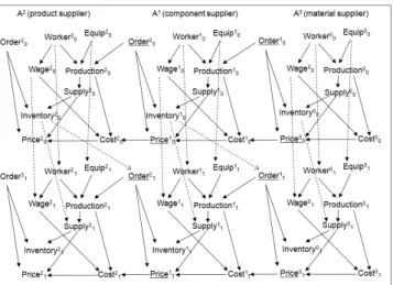
Fig. 4 illustrates such a multiagent system of three agents over two time intervals. Spatial dependences are along the horizontal direction and temporal evolution is along the ver-tical direction. For each supplier, availability of skilled workers, adequate equipment, and material (or component) ordered constrain the level of production, which in turn determines the amount of supply produced and influences the unit cost. Availability of skilled workers influences the workers’ wage, which in turn affects the unit cost. The unit cost is also affected by the sale price of the material from the next supplier down the chain. The amount of supply and the order incoming from the next supplier up the chain de-termine the inventory left and affect the unit sale price.

Figure 4: A DMSBN based multiagent system. Temporally, the current availability of workers, the cur-rent workers’ wage level, and the curcur-rent availability of

ade-quate equipment are closely dependent on their status in the previous time interval. Inventory left from the previous time interval affects both the current level of supply and the order of material from the next supplier down the chain.

Forecasting Algorithms

Forecasting proceeds as follows: At timei= 0, agents com-municate through the MSBN M0 to acquire prior for their respective subdomains. So each agentAj _{acquires a prior}

P( ˆV₀j)fori= 0.

Then each agentAj acquires observationsobsj₀ and up-dates its belief about its subdomain Vˆ₀j to get a posterior P( ˆV₀j|obsj₀) for i = 0. Due to d-sepset agent interface and interface observability, this step can be performed at each agent’s local JT without communication. After this the MSBNM1 is loaded into agents. The subnet forVˆ₁j is separated from the subnet forVˆ₀jthrough the forward inter-face, and a prior over the temporal interface is defined from a marginalization ofP( ˆV₀j|obsj₀). Through the MSBNM1, agents communicate and forecast fori = 1. That is, each agent Aj _{obtains the prior} _P_{( ˆ}_Vj

1|obs0)for i = 1, where obs0includes observations ati= 0by all agents.

From then on at each i, each agent Aj acquires obser-vationsobsj_i and updates its belief about its subdomain Vˆ_ij to get the posterior P( ˆV_ij|obsj₀, ..., obsj_i). It is performed at each agent’s local JT without communication. After this the MSBNMi+1is loaded into agents. The subnet forVˆij+1 is separated from the subnet for Vˆ_ij through a temporal interface, and a prior over the interface is obtained from marginalization ofP( ˆV_ij|obs₀j, ..., obsj_i). UsingMi+1with the priors, agents communicate and forecast fori+ 1. Each agentAjobtains the priorP(V_ij₊₁|obs0, ..., obsi)fori+ 1.

The above is enabled through a compilation of the DMSBN. Its subnets for each timei are compiled into an LJF and reused for each time instance. The compilation is similar to that for MSBNs, except that for each subnet of timei,F I_ij−1is contained in a cluster in the local JT and so isF I_ij. We denote the local JT of agentAj _{compiled from}

its subnetS_ijbyT_ij.

We assume that no forecast is made for the intervali= 0. The following diagram illustrates agent activities and their timing. The first line shows a sequence of time intervals each bounded by a pair of vertical bars. In the second line, the labelobs0 refers to local observation made during interval 0, and the label f orecast1 refers to forecasting on interval 1. The observation and forecasting activities are grouped into two algorithms InitialObservation and Forecast specified below. The third line illustrates which activities in the 2nd line are included in the execution of each algorithm.

| interval0 | interval1 | interval2 |... obs0 f orecast1 obs1f orecast2 obs2f orecast3... < Init >< F orecast >< F orecast > ...

(5)

Algorithm 1 (InitialObservation) At start of interval 0,

each agentAj_{does the following:}

1 load local JTT₀jinto memory;

2 enter local observations from interval0; 3 perform UnifyBelief;

Algorithm 2 (Forecast) At end of interval i ≥ 0, each agentAjdoes the following:

1 retrieve potentialB(F I_ij)from its local JTT_ij; 2 replaceT_ijbyT_ij₊₁in memory;

3 find a clusterQinT_ij₊₁such thatQ⊇F I_ij;

4 update potentialB(Q)intoB0(Q) =B(Q)∗B(F I_ij); 5 respond to call on CommunicateBelief;

6 answer forecasting queries on intervali+ 1; During intervali+ 1,Aj_{does the following:}

7 enter local observations from intervali+ 1; 8 perform UnifyBelief;

Note that for eachx∈F I_ij−1in the subnetS

j

i, it has no

parent inS_ij and is assigned a constant distribution. Hence, B(F I_ij₋₁)inT_ijis a constant distribution immediately after the local JT is loaded into memory.

CommunicateBelief is called upon an arbitrary agent during each interval.

Theorem 1 After execution of InitialObservation at each

agent, followed by Forecast from interval 0toi−1, fol-lowed by the first 6 lines of Forecast at end of intervali, the answers from each agent to forecasting queries on interval

i+ 1are exact.

Proof: We prove this by induction on time intervals. During InitialObservation, the LJF loaded in line 1 is globally consistent. In line 2, observations are entered at each agent. As agent interfaces are d-sepsets and due to interface observability assumption, each (enlarged) subdo-mainVˆ₀j is conditionally independent on each other subdo-mainVˆk

0 wherek6=j, given observations on an agent inter-face between them. Therefore, line 3 is equivalent to Com-municateBelief without actual communication. After line 3, not only each local JTT₀j is locally consistent, but also the LJF at interval 0 is globally consistent. From Theorem 8.121_{in (Xiang 2002), and the fact that}_{F I}j

0is contained in a single cluster inT₀j,B(F I₀j)retrieved from a unique cluster inT₀jis exact: That is,

B(F I₀j) =const∗P(F I₀j|obsj₀) =const∗P(F I₀j|obs0), where ‘const’ is a constant,obsj₀is the local observation by Aj ati= 0, andobs0includes observations ati= 0by all agents.

For the base casei = 0, we need only to consider one execution of the first 6 lines of Forecast at each agent. Based

1

Briefly, after agents enter their local observations,

Communi-cateBelief renders cluster potentials in each local JT to be exact

posteriors.

on the above argument,B(F I₀j)retrieved at line 1 is exact. At line 2, the LJF for i = 1 is loaded. From Lemma 1, marginalization of B(Q)toF I₀j is a constant distribution. Therefore, before line 4 is executed,B(Q) =const∗P(Q\

F I₀j|F I₀j), and the potential associated with local JTT₁j is B( ˆV₁j) =const∗P( ˆV₁j\F I₀j|F I₀j). After line 4 is executed, the potential overQbecomes

B0(Q) =const∗P(Q\F I₀j|F I₀j)∗P(F I₀j|obsj₀) =const∗P(Q|obsj₀).

This implies that the potential over T₁jbecomes

B0( ˆV₁j) =const∗P( ˆV₁j\F I₀j|F I₀j)∗P(F I₀j|obsj₀) =const∗P( ˆV₁j|obsj₀).

That is, the potential over T₁j has been conditioned on ob-servation obsj₀. This, however, makes the LJF fori = 1

inconsistent. After line 5, from Theorem 8.12 in (Xiang 2002), the LJF for i = 1 is again globally consistent and B0_{( ˆ}_Vj

1) =const∗P( ˆV

j

1|obs0). Hence, forecasting oni= 1 at line 6 is exact. This concludes the proof for the base case. Assume that the theorem holds when i = m. That is, when line 6 of Forecast is executed at end of intervalm, the LJF fori=m+ 1is globally consistent and, for eachAj,

B0( ˆV_mj₊₁) =const∗P( ˆV_mj₊₁|obs0, ..., obsm).

Hence, forecast oni=m+ 1is exact.

We consider intervali =m+ 1. First, each agent com-pletes lines 7 and 8 with respect to the LJF for interval m+ 1. Due to d-sepset agent interfaces and interface ob-servability, each subdomainVˆ_mj₊₁is conditionally indepen-dent on each other subdomain Vˆmk+1 wherek 6= j, given observations on an agent interface between them at inter-valsi= 0,1, ..., m, m+ 1. Therefore, line 8 is equivalent to CommunicateBelief. After line 8, the LJF for interval m+ 1is globally consistent, andB(F I_mj₊₁)retrieved from T_mj₊₁in line 1 during next execution of Forecast satisfies

B(F I_mj₊₁) =const∗P(F I_mj₊₁|obsj₀, ..., obsj_m, obsj_m₊₁). At line 2, the LJF fori=m+ 2is loaded by agents. After line 4, the potential overT_mj₊₂becomes

B0( ˆV_mj₊₂) =const∗P( ˆV_mj₊₂|obsj₀, ..., obsjm, obs j m+1), and the LJF fori=m+ 2is inconsistent. After line 5, the LJF is again globally consistent and B0( ˆV_mj₊₂) = const∗

P( ˆV_mj₊₂|obs0, ..., obsm, obsm+1). Hence, forecast at line 6 oni=m+ 2is exact.

Experiments

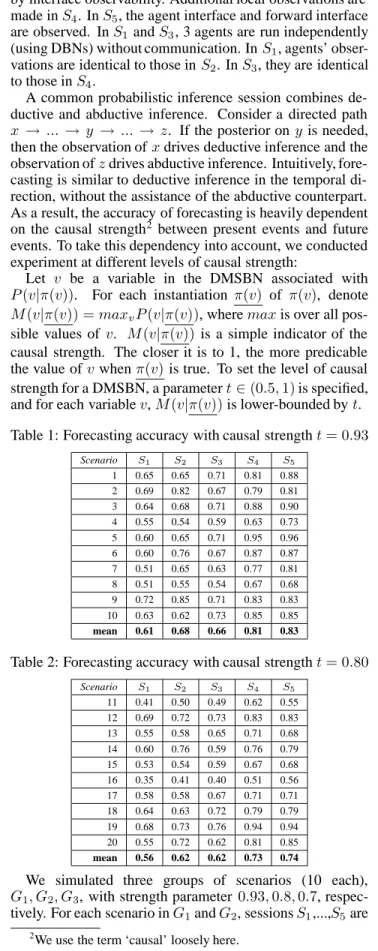
The 3-agent supply chain DMSBN in Fig. 4 and the equiv-alent centralized DBN are implemented using WebWeavr-IV. Each batch of experiment is conducted on a group of ten scenarios each of horizon 7, simulated from the DBN. For each scenario, five forecasting sessions (S1,...,S5) may be run. S2,S4 andS5 are run using the DMSBN. In S2,

(6)

only variables in agent interfaces are observed as assumed by interface observability. Additional local observations are made inS4. InS5, the agent interface and forward interface are observed. InS1andS3, 3 agents are run independently (using DBNs) without communication. InS1, agents’ obser-vations are identical to those inS2. InS3, they are identical to those inS4.

A common probabilistic inference session combines de-ductive and abde-ductive inference. Consider a directed path x → ...→ y → ... → z. If the posterior ony is needed, then the observation ofxdrives deductive inference and the observation ofzdrives abductive inference. Intuitively, fore-casting is similar to deductive inference in the temporal di-rection, without the assistance of the abductive counterpart. As a result, the accuracy of forecasting is heavily dependent on the causal strength2 _{between present events and future} events. To take this dependency into account, we conducted experiment at different levels of causal strength:

Let v be a variable in the DMSBN associated with P(v|π(v)). For each instantiation π(v) of π(v), denote M(v|π(v)) =maxvP(v|π(v)), wheremaxis over all

pos-sible values of v. M(v|π(v)) is a simple indicator of the causal strength. The closer it is to 1, the more predicable the value ofv whenπ(v)is true. To set the level of causal strength for a DMSBN, a parametert∈(0.5,1)is specified, and for each variablev,M(v|π(v))is lower-bounded byt. Table 1: Forecasting accuracy with causal strengtht= 0.93

Scenario S1 S2 S3 S4 S5 1 0.65 0.65 0.71 0.81 0.88 2 0.69 0.82 0.67 0.79 0.81 3 0.64 0.68 0.71 0.88 0.90 4 0.55 0.54 0.59 0.63 0.73 5 0.60 0.65 0.71 0.95 0.96 6 0.60 0.76 0.67 0.87 0.87 7 0.51 0.65 0.63 0.77 0.81 8 0.51 0.55 0.54 0.67 0.68 9 0.72 0.85 0.71 0.83 0.83 10 0.63 0.62 0.73 0.85 0.85 mean 0.61 0.68 0.66 0.81 0.83

Table 2: Forecasting accuracy with causal strengtht= 0.80 Scenario S1 S2 S3 S4 S5 11 0.41 0.50 0.49 0.62 0.55 12 0.69 0.72 0.73 0.83 0.83 13 0.55 0.58 0.65 0.71 0.68 14 0.60 0.76 0.59 0.76 0.79 15 0.53 0.54 0.59 0.67 0.68 16 0.35 0.41 0.40 0.51 0.56 17 0.58 0.58 0.67 0.71 0.71 18 0.64 0.63 0.72 0.79 0.79 19 0.68 0.73 0.76 0.94 0.94 20 0.55 0.72 0.62 0.81 0.85 mean 0.56 0.62 0.62 0.73 0.74

We simulated three groups of scenarios (10 each), G1, G2, G3, with strength parameter 0.93,0.8,0.7, respec-tively. For each scenario inG1andG2, sessionsS1,...,S5are

2

We use the term ‘causal’ loosely here.

run. For each scenario (of horizon 7), six forecastings are made. The accuracy over 13 variables (distributed among agents) in each forecasting is recorded. Tables 1 and 2 show the average accuracy over13×6 = 78variables.

By comparing results between S1 andS2, and between S3 andS4, it can be seen that DMSBN agents have more accurate forecasting than DBN agents. By comparing results betweenS1 andS3, and betweenS2,S4 andS5, it can be seen that more observations result in more accurate forecasts by both DBN and DMSBN agents.

In addition, we run session S5 for each scenario inG3, and the average accuracy over 10 scenarios is 0.53. From the average accuracies ofS5inG1,G2andG3, i.e., 0.83, 0.74 and 0.53, respectively, it is clear that stronger causal strength in the environment results in more accurate forecasting.

Acknowledgements

We acknowledge the financial support from Discovery Grant, NSERC, Canada, to the first author, and funding from EPSRC CRiSM Initiative through the second author.

References

An, X.; Xiang, Y.; and Cercone, N. 2008. Dynamic multiagent probabilistic infer-ence. International Journal of Approximate Reasoning 48(1):185–213.

Brockwell, P., and Davis, R. 1991. Time Series: Theory and Methods (2nd Ed.). Springer, New York.

Dahlhaus, R., and Eichler, M. 2003. Causality and graphical models for time se-ries. In Green, P.; Hjort, N.; and Richardson, S., eds., Highly Structured Stochastic Systems. Oxford University Press. 115–137.

Dean, T., and Kanazawa, K. 1989. A model for reasoning about persistence and causation. Computational Intelligence 5(3):142–150.

Kiekintveld, C.; Miller, J.; Jordan, P.; and Wellman, M. 2007. Forecasting market prices in a supply chain game. In Proc. 6th inter. joint conference on autonomous agents and multiagent systems, 1–8. ACM.

Kjaerulff, U. 1992. A computational scheme for reasoning in dynamic probabilistic networks. In Dubois, D.; Wellman, M.; D’Ambrosio, B.; and Smets, P., eds., Proc. 8th Conf. on Uncertainty in Artificial Intelligence , 121–129.

Koller, D., and Lerner, U. 2001. Sampling in factored dynamic systems. In Doucet, A.; de Freitas, J.; and Gordon, N., eds., Sequential Monte Carlo in Practice , 445– 464. Springer-Verlag.

Lauritzen, S. 1996. Graphical Models. Oxford.

Pearl, J. 1988. Probabilistic Reasoning in Intelligent Systems: Networks of Plausible Inference. Morgan Kaufmann.

Pournara, I., and Wernisch, L. 2004. Reconstruction of gene networks using Bayesian learning and manipulation experiments. Bioinformatics 20(17):2934– 2942.

Queen, C., and Smith, J. 1993. Multi-regression dynamic models. J. Roy. Statist. Soc. Ser. B 55(4):849–870.

Raudys, S., and Zliobaite, I. 2006. The multi-agent system for prediction of financial time series. In Artificial Intelligence and Soft Computing - ICAISC 2006, LNCS 4029. Springer. 653–662.

West, M., and Harrison, P. 1996. Bayesian Forecasting and Dynamic Models (2nd Ed). Springer.

Xiang, Y. 1998. Temporally invariant junction tree for inference in dynamic Bayesian network. In Mercer, R., and Neufeld, E., eds., Advances in Artificial Intel-ligence. Springer. 363–377.

Xiang, Y. 2002. Probabilistic Reasoning in Multiagent Systems: A Graphical Mod-els Approach. Cambridge University Press, Cambridge, UK.