Error voltage based open switch fault diagnosis strategy for matrix converters with model predictive control method

Error-Voltage Based Open-Switch Fault Diagnosis

Strategy for Matrix Converters with Model Predictive

Control Method

Abstract—This paper proposes an error-voltage based open-switch fault diagnosis strategy for matrix converter (MC). A finite control set model predictive control (FCS-MPC) method is used to operate the MC. The MC system performances under normal operation and under a single open-switch fault operation are analyzed. A fault diagnosis strategy has also been implemented in two steps. First, the faulty phase is detected and identified based on a comparison of the reference and estimated output line-to-line voltages. Then, the faulty switch is located by considering the switching states of the faulty phase. The proposed fault diagnosis method is able to locate the faulty switch accurately and quickly without additional voltage sensors. Simulation and experimental results are presented to demonstrate the feasibility and effectiveness of the proposed strategy. 1

Keywords—Fault diagnosis; finite control set model predictive control; matrix converter; single open-switch fault

I. NOMENCLATURE source voltage

source current input voltage

max min

input current

output phase voltage [ ] actual output line-to-line voltage [ ] reference output line-to-line voltage [ ] estimated output line-to-line voltage [ ]

load current [ ] line-to-line load current [ ]

∗ _{source current reference [} ∗ ∗ ∗_] ∗ _{load current reference [} ∗ ∗ ∗ _]

prediction of source current [ ] prediction of load current [ ]

1

Manuscript received January 1, 2017; revised February 26, 2017; accepted April 10, 2017. This work was supported by the Major Program of the National Natural Science Foundation of China under Grant 61490702, the China Scholarship Council under Grant 201606370137.

amplitude of source phase voltage

∗ _{amplitude of source current reference} ∗ _{amplitude of load current reference}

∅ the angle of the source current phase shift between the source voltage and current

the angle of the load current output active power

input active power filter resistance filter inductance filter capacitance load resistance load inductance the sampling period the capacitor voltage of the clamp circuit

II. INTRODUCTION

Matrix converters (MCs) are a promising family of direct AC-AC power electronic converters. Compared with the conventional power converters, the matrix converter possesses the advantages of bi-directional power flow with full four-quadrant operation, sinusoidal input and output currents, controllable input power factor, high power density and no DC-link energy storage elements [1]-[3]. Nevertheless, the components of MC may suffer several kinds of electrical faults. These components include capacitors, printed circuit boards (PCBs), semiconductor devices, solder joints, and connectors [4]-[5]. Among them, the power device module is the most vulnerable component, reportedly accounting for 34% of failures in converter systems (21% of semiconductor and 13% of solder joint) [6]. The failure of power device can be classified as open circuit failure and short circuit failure [7]. As a protection circuit is always installed in MC system, a fast fuse in series with each of the switches can be employed when a short circuit fault occurs, then a short circuit failure is changed into an open circuit failure. When an open-switch fault occurs in one phase of the MC as shown in Fig. 1, the clamp circuit has to conduct the current that originally flowed through the faulty phase, and then the clamp voltage will be

Patrick Wheeler

Department of Electrical and Electronics Engineering The University of Nottingham, Nottingham, UK

[email protected]

Hanbing Dan, Tao Peng, Mei Su, Hui Deng,

Qi Zhu, Ziyi Zhao,

School of Information Science and Engineering Central South University, Changsha, China

enlarged. This would accelerate the damage in a normal switch and lead to the occurrence of a secondary fault. If the faulty switch is not located in time, fault tolerant operation of the MC [8]-[9] cannot follow the isolating of the faulty switch. Therefore, issues, including real-time monitoring of the operating state and fault diagnosis of the MC, are gradually brought into sharp focus due to the demands for high reliability and lifetime.

In the existing literature, the methods for diagnosing an open-switch fault in power converters can be divided into two types: the signal processing-based approach and the analytical model-based approach [10]. For the signal processing-based approach in a MC system, the discrete wavelet transform analysis of measured output current is an example of a fault diagnosis method [11]. However, the diagnosis time is long if the fault occurs near the zero crossing of the faulty phase current. The analytical model-based approach for MC systems can be seen in [12]-[18]. In [12], the faulty phase is identified under the condition when the load current is equal to zero for 30 consecutive sampling periods. Then an additional algorithm is used to locate the faulty switch. In [13], the fault diagnosis method is proposed for Alesina-Venturini (AV). The diagnosis approach utilizes the special feature of the AV method, such as the load currents, the angles of the input and output voltage space vectors, and the duty cycles of the switches. However, these fault diagnosis methods in [12]-[13] require relatively long detection times. In [14], a fault diagnosis method based on the analysis of the currents circulating through the drive system is presented. This method can detect the faulty switch within a minimum of one switching period, in the example given about 0.08 ms after the fault occurs. However, an additional current sensor is needed to monitor the clamp current.

To reduce the detection time and avoid additional sensors, the fault diagnosis method in [15] moves the load current sensors ahead of the clamp circuit connection. This arrangement detects and locates the faulty switch according to the information from the current sensors during the zero vectors. The accurate detection of the current sensor depends on an adequate zero vector time. This method is therefore not fit for MC applications where a high voltage transfer ratio is needed as the zero vector time will be small.

In [16], the proposed fault recognition method can detect and locate the faulty switch with voltage error signals dedicated to each switch, based on a direct comparison of the input and the output voltages. In [17]-[18], the differences between the measured and predicted output voltages are used as the criterion for the diagnosis. However, the diagnosis methods in [16]-[18] require additional voltage transducers and analog to digital converters (ADC) with a very high bandwidth, which adds the system cost.

The finite control set model predictive control (FCS-MPC) has been shown to be a very interesting alternative for the modulation and control of MCs [19]-[21]. It uses the time-discrete model of the MC topology to predict the future

values of, for example, the load currents and decides the most suitable switching state for the next sampling period. The FCS-MPC possesses several advantages, such as fast dynamic response, easy inclusion of nonlinearities and constraints of the system [22]-[24]. Currently, the fault diagnosis for the MC with FCS-MPC has not been considered in depth.

In [25] a fault diagnosis method for MCs is proposed which monitors the load currents and considers the switching state to locate the faulty switch. It is simpler to diagnose the exact location of the open-circuit switch in a MC with FCS-MPC. However, it is difficult to diagnosis the open-circuit fault switch when the following two conditions are satisfied simultaneously: i) The frequency of the load current is same with the frequency of the input voltage. ii) The phase difference between the input voltage and the output current isπ. The current-based fault diagnosis [25] has been proposed for MC with FCS-MPC. However, voltage-based fault diagnosis strategy for MC with FCS-MPC has not been considered but may have some important advantages. Ideally, the fault diagnosis strategy should be accomplished without increasing the overall system cost and complexity. Thus, this paper uses the load model to estimate the actual output line-to-line voltage. The reference output line-to-line voltage is obtained from the input voltage and the switching states. Then the difference between the estimated output line-to-line voltage and the reference output line-to-line voltage is used to detect an open-circuit fault. The switching state is utilized to locate the faulty switch. Therefore, the additional hardware and large computational burdens are avoided. In addition, the advantages of voltage-based fault diagnosis, such as fast detection and an inherent high immunity to the false alarms, are inherited. The proposed fault diagnosis method in this paper has been described in [26], more principle details and experimental results are added in this paper.

This paper is organized as follow. In Section II, the normal operation based on FCS-MPC is presented. In addition, the MC performance under open-switch fault operation is analyzed. Then, in section III, the fault diagnosis method is described in detail. Finally, simulation and experimental results are presented to demonstrate the feasibility of the proposed strategy.

III. MC SYSTEM

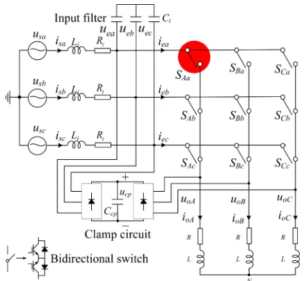
The matrix converter topology is shown in Fig. 1. The circuit consists of nine bi-directional switches, an input filter, and a clamp circuit. The bi-directional switches connect a three phase voltage source to a three phase resistance-inductance load for bi-directional energy flow. The input filter filters the switched input current of the converter to attenuate the switching frequency harmonics. The clamp circuit consists of 12 fast-recovery diodes to connect the clamping capacitor between the input and output terminals, to avoid overvoltage coming from the grid side and the load side.

[image:3.595.53.273.51.254.2]

Fig. 1. Matrix converter topology.

prohibited between the input lines, respectively. The switching states of each load phase must satisfy

+ + =1

+ + =1

+ + =1

Aa Ab Ac

Ba Bb Bc

Ca Cb Cc

S S S

S S S

S S S

     (1)

where SXy (X ∈ {A, B, C}, y ∈ {a, b, c}) equals to ‘1’ when

switch SXy is turned on and equals to ‘0’ when switch SXy is

turned off, respectively. So the MC can generate 27 valid switching states. The reference output line-to-line voltages and input currents can be obtained as follows

1

1

1

oAB Aa Ba Ab Bb Ac Bc ea

oBC Ba Ca Bb Cb Bc Cc eb

oCA Ca Aa Cb Ab Cc Ac ec

u S S S S S S u

u S S S S S S u

u S S S S S S u

          _ _{  }                         (2) T

ea Aa Ab Ac oA

eb Ba Bb Bc oB

ec Ca Cb Cc oC

i S S S i

i S S S i

i S S S i

       _                      (3)

For the sake of completeness of this paper and for an easy understanding of the faulty operation of an MC, the FCS-MPC that rules the normal operation of an MC will be presented firstly. Then, the faulty operation of MC with an open-switch fault is analyzed.

A. Normal Operation with FCS-MPC [27]

The continuous-time models of input filter and load are given as follow

e

e s

s e

s

d

dt _{A B}

d dt                           u u u i i

i (4)

o

o o

d

L R

dt  

i

u i (5) where

0 1 / 0 1 /

1 / / 1 / 0

i i

i i i i

C C

A B

L R L L

     _{ } _{ }       (6) Then, the discrete models are achieved as

1

1

k k k

e e s

k k k

s s e

G H                      

u u u

i i i (7) 1

(1 )

k s k s k

o o o

T T R

L L



  

i u i (8) where

AT_s

Ge ,

H



A



1

(

G I B



)

(9) To obtain the desired load currents and unity power factor for the MC, the following cost function is used.

2 2

* *

* _oP _{o s}P _s

g i i  i i (10) where the weighting factor λ is empirically adjusted [28]. The predicted values of the load currents and the source currents can be obtained according to (7) and (8), respectively. The reference value of load current is given by

* * * *

o cos cos( 2 / 3) cos( 2 / 3)

T

o_I m  Iom   Iom   _

i (11)

The reference value of source current is given as follow

* * * *

cos cos( 2 / 3) cos( 2 / 3) T

s _Ism  Ism   Ism   _

i (12)

The input and output active powers are calculated from (13) to (15).

* 2 3 2

o om

P  I R (13)

* * 2

3 (

cos

)

2

in sm sm sm i

P



U I





I

R

(14) o

in

P P



 (15) where η denotes the system efficiency.

Hence, the amplitude of the expected source current ∗ can be calculated as [27]





2 * 2

* 4

2

sm sm i om

sm

i

U U R I R

I R        

 (16)

At each sampling period, the cost function values of 27 valid switching states are calculated. Finally, according to the following equation, the switching state N that produces the minimum value is applied in the next sampling period.

g[ ]

N



min{ [1], [2],

g

g



, [ ],

g i



, [27]}

g

(17) B. Single Open-Switch Fault Operation

voltage, the input filter is ignored to simply the analysis in the equivalent circuit. The arrow in Fig. 1 specifies the direction of positive load phase current flow. Assume that switch is suffering an open-switch fault and is applied. When the direction of load phase-A current is positive, the output terminal of load phase-A will be connected to the negative terminal of the capacitor in clamp circuit. The corresponding equivalent circuit is shown in Fig. 2 (a). When the direction of load phase-A current is negative, the output terminal of load phase-A will be connected to the positive terminal of the capacitor in clamp circuit. The corresponding equivalent circuit is shown in Fig. 2 (b). Thus, the actual output phase voltages are expressed as follow

max

emin

, 0

, 0

oA cp oA

oA cp oA

ea

oB Ba Bb Bc

eb

Ca Cb Cc

oC

ec

u u u faulty i

u u u faulty i

u

u S S S

u

S S S

u

u

  

  

 

   _{  }



   _{  }

 

  _{ }

 

，

， (18)

The actual output line-to-line voltages are achieved as

(a)

(b)

Fig. 2. The equivalent circuit when switch is suffering an open-switch fault and is applied. (a) Load phase-A current >0, (b) Load phase-A current

<0.

emax

emin

emax

emin

, , 0

, , 0

( ) ( )

( )

, 0

, 0

oAB cp oB oA

oAB cp oB oA

oBC Ba Ca ea Bb Cb eb

Bc Cc ec

oCA cp oC oA

oCA oC cp oA

u u u u faulty i

u u u u faulty i

u S S u S S u

S S u

u u u u faulty i

u u u u faulty i

   

 

   



 _{   }

 

 



 _{   }



   

 

(19)

Meanwhile, since the load phase-A current charges the capacitor of the clamp circuit, the capacitor voltage of the clamp circuit is larger than the maximum input line-to-line voltage. Under normal operation, the actual output line-to-line voltage will be same with the reference value . If is suffering an open-switch fault and is applied, the actual output line-to-line voltage and will be different from the reference value and according to (2) and (19). This feature can be exploited later for fault detection.

[image:4.595.315.547.305.667.2]

To obtain the output line-to-line voltage without requiring extra voltage sensors, the load model is built as follow

[image:4.595.66.262.327.644.2]

o

o

o

0

oA

A oA N

oB

B oB N

oC

C oC N

oA oB oC

di

u Ri L u

dt di

u Ri L u

dt di

u Ri L u

dt

i i i

       _{  }              (20)

where is the voltage between the load neutral point and the ground point of the power supply.

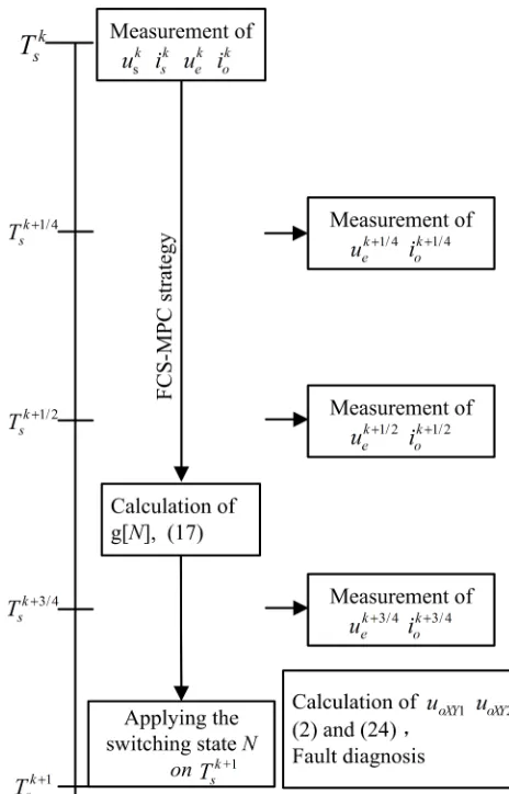
According to (20), the actual output line-to-line voltage can be estimated if the derivative part of the load current is known. In order to obtain an accurate derivative part of the load current, the load currents are sampled four times in a sampling period as shown in Fig. 3. The sampling values at and the known switching state at kth sampling period are used for calculation of variables at . Then, all switching states are applied for prediction of variables at . The switching state making the cost function minimum will be applied in the (k+1)th sampling period. The sampling values at / ,

/

and / are used for estimation of the output line-to-line voltage. Since the switching state stays the same from to , the sampling values will not be disturbed by the four-step current-based commutation [29]. Assume output load current is

( ) oX( ) ( , , )

f t i t XA B C (21) According to Taylor’s formula, the following equations can be obtained.

s s s s

s s

s s s s

s s '

s 4 s 2 s 2 4

( )

s 2 4

3 '

s 4 s 2 s 2 4

( )

s 2 4

( + ) ( + ) ( + ) * ( ) ( + ) * ( ) ( + ) ( + ) ( + ) * ( )

( + ) * ( )

T T T T

T T

n n

T T T T

T T

n n

f kT f kT f kT

f kT

f kT f kT f kT

f kT             (22)

When the high order part ∑ ( ) _{kT + ∗ ( )}

, … is

neglected, the derivative part of the load current is obtained as follow

s s s

s s

3

' 2 2

s 2 s 4 s 4

( +T) _T ( + T) _T ( +T)

f kT  f kT  f kT (23)

Compared with the common method, equation (23) is more accurate to the true value with consideration of the second order part of the load current. The actual output line-to-line voltages are estimated by substituting (23) into (20) as follow

1/ 2 2 3/ 4 1/ 4

o o 2

1/ 2 2 3/ 4 1/ 4

o o 2

1/ 2 2 3/ 4 1/4

o o 2

( ) ( ) ( ) s s s

k L k k

AB AB oAB T oAB oAB

k L k k

BC BC oBC T oBC oBC

k L k k

CA CA oCA T oCA oCA

u u Ri i i

u u Ri i i

u u Ri i i

                            (24) where =

1 / 4, =

1 / 2, 3 / 4 =

j j j

oAB oA oB

j j j

oBC oB oC

j j j

oCA oC oA

i i i

j k

i i i

k k

i i i

              (25)

By the way of monitoring the load currents based on (24), the actual output line-to-line voltages under faulty operation are estimated without additional voltage sensors.

In addition, the reference output line-to-line voltage is obtained from the input voltage and the switching states according to (2). Note that to suppress the disturbance, the mean value of input voltage in (2) is obtained as follow

1/ 4 1/ 2 3/ 4 1

e 3( )

k k k

e e e

u  u  u  u  (26) IV. FAULT DIAGNOSIS METHOD

From the discussion in the previous section, the output line-to-line voltages under faulty operation are not equal to the reference values. Based on these observations, this section proposes a fault detection algorithm which uses two steps to identify the fault. The first step detects the occurrence of the fault and identifies the faulty phase. The second step locates the faulty switch.

A. Step 1: Detection and Identification of the Open-Circuit Phase

Three error voltages , and are defined as the residuals, which are shown as

o 1 o 2

o 1 o 2

oC 1 oC 2

AB AB AB

BC BC BC

CA A A

u u u u u u               (27)

Under normal conditions, the output line-to-line voltages equal to their reference values. As a result, the residuals of the output line-to-line voltage are ideally zero (in practical cases, they are expected to be a very small valuedue to the voltage drop across the IGBTs in a conducting state, the dead time of switch commutation, etc.). The residuals are within a small threshold. When single open-switch fault occurs at the switch , the value of the output phase voltage with respect to the supply neutral will change. It will be equal to either the positive or the negative DC-bus voltage of the clamp circuit according to the direction of the output phase current. The residuals related to the faulty output phase are shown as

emax

emin

, 0 , 0

ey cp oX

XY

ey cp oX

u u u for i

u u u for i

             (28)

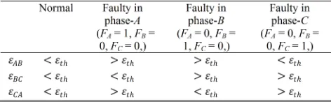
where X, Y ∈ {A, B, C},  , y ∈ {a, b, c}. The residuals related to the faulty output phase will exceed a threshold. While the residual of thetwonormal output phases preserves a low value.

TABLEI RESIDUALS UNDER NORMAL AND FAULTY SITUATIONS

under normal and faulty situations are illustrated. FX (X ∈ {A,

B, C}) equals to ‘1’ whenthe load phase-X is faulty and equals to ‘0’ when the load phase-X is normal.

B. Step 2: Location of the Open-Circuit Switch

After the detection and recognition of faulty phase, the open-circuit switch must be located. For the MC with FCS-MPC, the switching state taken in a sampling period is clear and constant. In addition, only one switch is turned on for connecting each output phase to the input phase. Therefore, the switch which connects the faulty phase to the input phase is located as the open-circuit switch. The algorithm to locate the open-circuit switch after identifying the faulty phase is presented as follow

0 0

0 0

0 0

Aa Ab Ac A Aa Ab Ac

Ba Bb Bc B Ba Bb Bc

Ca Cb Cc C Ca Cb Cc

F F F F S S S

F F F F S S S

F F F F S S S

     

 _   

     

     

     

(29)

Where (X ∈ { , , }, ∈ { , , }) equals to ‘1’ when is open-circuit and equals to ‘0’ when is normal. For example, if ( > )&&( < ) &&( > ), from Table I, = 1, = 0, = 0, and the current switching state is = 1, = 0, = 0. According to (29), = 1. As a result, is regarded as the open-circuit switch.

The described technique employs a direct comparison between the reference and estimated output line-to-line voltages to locate the open-circuit switch, without any requirement of additional voltage sensors. Thus, for the improvement of the MC reliability, based on the proposed detection and identification of the failed switch, fault tolerant operation of the MC drive systems can be followed by isolating the faulty devices.

V. SIMULATION RESULTS

To verify the effectiveness of the proposed fault diagnosis method, some numerical simulations are carried out by using Matlab/Simulink. All the components of MC topology used in the simulation are chosen from the power system block set in the Simulink and the dead time of the device is not taken account. The corresponding component parameters are indicated in Table II. To make the fault diagnosis method more robust and to minimize the possibility of the false alarms, a positive threshold is selected, which is 60V in the simulation.

Fig. 4 and Fig. 5 show the simulation results of the MC system with ∗ = 10A, = 30Hz during normal and faulty operation when the fault diagnosis and tolerant methods

TABLEII PARAMETERS OF THE SIMULATION

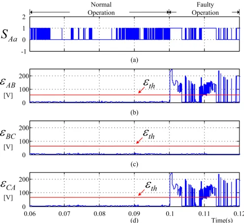
are unused. As shown in Fig. 4, during normal operation, the MC system is operated with FCS-MPC, which employs a time-discrete model of the MC topology and a cost function to select the best switching state for the next sampling period. Three load currents are seen to be sinusoid with low distortions. In addition, the estimated line-to-line voltage is nearly equal to the reference output line-to-line voltage. During faulty operation, the fault is simulated by imposing permanent zero gate signals to both IGBTs belonging to switch . The load phase-A current is distorted and rapidly decreased to zero after the open circuited fault of occurs at t= t1, the load phase-B current and load phase-C current are also affected. In addition, since the actual line-to-line voltage is not the reference output line-to-line voltage, the estimated output line-to-line voltage is different from the reference output line-to-line voltage. As shown in Fig. 5, during normal operation, three residual errors , and

are all below the threshold value. During faulty operation, residual error is below the threshold value, while residual errors and are above the threshold value when predictive controller intends to give “ON” signal to . This phenomenon above is used for the fault diagnosis.

Fig. 6 and Fig. 7 show the simulation results of the MC system with ∗ = 10A, = 30Hz during normal and faulty operation when the fault diagnosis and tolerant methods are activated. The fault diagnosis method in Section IV is applied while the fault tolerant strategy in [25] is applied. The fault tolerant strategy selects the appropriate switching state for the remaining eight switches to minimize the error between the load current and the reference current. As shown in Fig. 6, during normal operation, three residual errors , and are all below the threshold value, and the fault detection signal remains zero. During faulty operation, when predictive controller intends to give “ON” signal to , a “OFF” signal is imposed to switch instead to simulate the open-circuit failure. Therefore, the load current flows through both the matrix converter and the clamp circuit. The actual output line-to-line voltage is different from the reference output line-to-line voltage. As a result, the residual errors and exceed the threshold. Three residual errors and the switch signal satisfy ( = 1)&&( >

[image:6.595.45.281.64.137.2] [image:6.595.328.540.64.172.2]

Fig. 4. Simulation results of the MC system with ∗ = 10A, = 30Hz during normal and faulty operation when the fault diagnosis and tolerant methods are unused. (a) The load current . (b) The load current . (c) The load current . (d) The reference output line-to-line voltage . (e) The estimated output line-to-line voltage .

Fig. 5. Simulation results of the MC system with ∗ _{= 10A, = 30Hz}

during normal and faulty operation when the fault diagnosis and tolerant methods are unused. (a) The gate signal of the switch . (b) The residual error . (c) The residual error . (d) The residual error .

Fig. 6. Simulation results of the MC system with ∗ _{= 10A, = 30Hz}

during normal and faulty operation when the fault diagnosis and tolerant methods are activated. (From t = 0.06 to t = 0.12) (a) The gate signal of the switch . (b) The residual error . (c) The residual error . (d) The residual error . (e) The faulty detection signal .

[image:7.595.309.558.53.336.2] [image:7.595.40.287.57.345.2] [image:7.595.308.561.398.683.2] [image:7.595.41.289.404.631.2]

switch . (b) The residual error . (c) The residual error . (d) The residual error . (e) The faulty detection signal .

VI. EXPERIMENTAL RESULTS

The error-voltage based fault diagnosis method is further evaluated on an experimental prototype. The experimental setup comprises nine bi-directional switches FF200R12KT3_E and a controller, whose core control chip is TMS320F28335 and EP2C8T144C8N. The load current is obtained by the current sensor LT208-S7. The analog-to-digital conversion (ADC) chip in the control board is MAX1308. The actual sample instant is about 100ns later than the desired sample instant. The impact of the delay during the ADC conversion process can be nearly neglected. The other parameters of the experimental setup are the same of the simulation parameters shown in Table II.

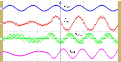
In order to ensure the load current regulation and unity power factor operation, the FCS-MPC technique is adopted to control the MC under normal condition. The experimentally measured result under normal condition is shown in Fig. 8, where the Ch1 trace is the actual source voltage ; the Ch2 trace is the actual source current ; the Ch3 trace is the actual output line-to-line voltage ; and the Ch4 trace is the actual load current . As shown in Fig. 8, when the reference load current changes from 6A/30Hz to 12A/60Hz, the unity input power factor is obtained and the actual load current tracks the reference load current. Fig. 9 also shows the experimentally measured results under the same condition as Fig. 8. In Fig. 9, the Ch1 trace is the actual load current ; the Ch2 trace is the reference output line-to-line voltage ; the Ch3 trace is the estimated output line-to-line voltage ; the Ch4 trace is the error voltage . It is clear that the reference output line-to-line voltage and estimated output line-to-line voltage are almost coinciding, and error voltage is less than 20V. In addition, there is no misdiagnosis, regardless the change of reference load current.

The error voltages , and in normal and faulty operation are compared in Fig. 10. Where the Ch1 trace is the actual load current ; the Ch2, Ch3 and Ch4 traces are error voltages , and respectively. As indicated in Fig. 10. Under normal operation, the error voltages , and are all less than 20V. Under faulty operation, when predictive controller intends to give “ON” signal to , a “OFF” signal is imposed to switch instead to simulate an open-circuit failure. Therefore, the load current flows through both the matrix converter and the clamp circuit. The error voltages and are both larger than 100V, while the error voltage is less than 20V. Thus, the different feature of the error voltages under normal and faulty operation can be used for the fault detection and location. The threshold error voltage is set as 60V according to the above analysis.

According to the above analysis, the fault diagnosis method in section IV is applied. As shown in Fig. 11 (a), an open-circuit fault is imposed on the switch at t=t1. The

load current in Ch1 is distorted after t=t1. Ch2, Ch3 and Ch4 show three residual errors , and between

, , based on known switching states and , , based on the load model. Since ( =

1)&&( > )&&( < ) &&( > ), the switch is diagnosed as the faulty switch. This phenomenon can be seen more clearly from the enlarged drawing of a dotted box in Fig. 11 (b). As indicated in Fig. 11 (b), the diagnosis time is only a sampling period time (100us). To obtain the better quality of the load current under faulty operation without additional hardware, the fault tolerant strategy in [25] is applied. To validate the universality of the proposed fault diagnosis method, the reference load current frequency is set as same as the source voltage frequency. The open-circuit fault switch in this condition is difficult to be detected for the fault diagnosis method in [25]. The experimental result for the proposed fault diagnosis method in this paper is shown in Fig. 12, where the Ch1 trace is the actual load current ; the Ch2, Ch3 and Ch4 traces are error voltages , and respectively. The faulty switch is also detected and located during a sampling period.

Fig. 8. Experimentally measured results of the MC system in the normal condition with the reference load current set from ∗ = 6A, = 30Hz to

∗ _{= 12A, = 60Hz. (Ch1: [250V/div], Ch2: [10A/div], Ch3: [250V/div],}

Ch4: [20A/div], Time: [10ms/div])

Fig. 9. Experimentally measured results of the MC system in the normal condition with the reference load current set from ∗ _{= 6A, = 30Hz to} ∗ _{= 12A, = 60Hz. (Ch1: [20A/div], Ch2: [200V/div], Ch3: [200V/div],}

[image:8.595.309.558.320.449.2] [image:8.595.309.558.498.626.2]

[image:9.595.41.289.56.194.2]

Fig. 10. Experimentally measured results of the MC system with ∗ _{= 10A,}

= 30Hz during normal and faulty operation when the fault diagnosis and tolerant methods are unused. (Ch1: [20A/div], Ch2: [250V/div], Ch3: [250V/div], Ch4: [250V/div], Time: [10ms/div])

(a)

(b)

Fig. 11. Experimentally measured results of the MC system with ∗ = 10A, = 30Hz during normal and faulty operation. (a) The fault diagnosis and tolerant methods are activated. (b) The enlarged drawing of the dotted box. (Ch1: [20A/div], Ch2: [250V/div], Ch3: [250V/div], Ch4: [250V/div])

(a)

[image:9.595.310.561.56.350.2]

(b)

Fig. 12. Experimentally measured results of the MC system with ∗ = 12A, = 50Hz during normal and faulty operation. (a) The fault diagnosis and tolerant methods are activated. (b) The enlarged drawing of the dotted box. (Ch1: [20A/div], Ch2: [250V/div], Ch3: [250V/div], Ch4: [250V/div])

VII. CONCLUSION

An error-voltage based open-switch fault diagnosis strategy for MCs controlled with a FCS-MPC method has been investigated. The error-voltage is obtained by comparing the reference output line-to-line voltage and the estimated output line-to-line voltage. The reference output line-to-line voltage is obtained based on the input voltage and known switching state, while the estimated output line-to-line voltage is obtained based on the load model. The proposed fault diagnosis strategy is cost-saving and space-saving because no additional voltage sensor is needed. In addition, compared with the fault diagnosis time 1.4ms in [25], the detection time of the proposed fault diagnosis strategy is only a sampling period (100us). Meanwhile, the high immunity to the false alarm is also guaranteed. Finally, simulation and experimental results demonstrate the feasibility and effectiveness of the error-voltage based open-switch fault diagnosis strategy.

REFERENCES

[1] L. Empringham, J. W. Kolar, J. Rodriguez, P. W. Wheeler, and J. C. Clare, “Technological issues and industrial application of matrix converters: a review,” IEEE Trans. Ind. Electron., vol. 60, no. 10, pp. 4260-4271, 2013.

[2] J. Rodriguez, M. Rivera, J. W. Kolar, and P. W. Wheeler, “A review of control and modulation methods for matrix converters,” IEEE Trans. Ind. Electron., vol. 59, no. 1, pp. 58-70, 2012.

[image:9.595.39.288.252.541.2]

and H. P. Krug, "Development of mcs and its applications in industry,"

IEEE Trans. Ind. Electron., vol. 5, pp. 4-12, 2011.

[4] U. M. Choi, F. Blaabjerg, S. Jorgensen, S. Munk-Nielsen, and B. Rannestad, “Reliability improvement of power converters by means of condition monitoring of igbt modules,” IEEE Trans. Power Electron., vol. pp, no. 99, pp. 1-1, 2016.

[5] S. Yang, A. Bryant, P. Mawby, D. Xiang, L. Ran, and P. Tavner, “An industry-based survey of reliability in power electronic converters,”

IEEE Trans. Ind. Appl., vol. 47, no. 3, pp. 1441–1451, May/Jun. 2011. [6] E. Wolfgang, “Examples for failures in power electronics systems,”

presented at ECPE Tutorial ‘Reliability of Power Electronic Systems’, Nuremberg, Germany, Apr. 2007

[7] R. Wu, F. Blaabjerg, H. Wang, M. Liserre, and F. Iannuzzo, " Catastrophic failure and fault-tolerant design of IGBT power electronic converters-an overview," in Proc. 2013 IEEE Industry Electronics Society Annual Conference, pp. 507-513.

[8] J. D. Dasika and M. Saeedifard, "A fault-tolerant strategy to control the matrix converter under an open-switch failure," IEEE Trans. Ind. Electron., vol. 62, pp. 680-691, 2015.

[9] S. Khwan-on, L. de Lillo, L. Empringham, and P. Wheeler, "Fault-tolerant matrix converter motor drives with fault detection of open switch faults," IEEE Trans. Ind. Electron., vol. 59, pp. 257-268, 2012.

[10] S. X. Ding, "Model-based fault diagnosis techniques design schemes, algorithms, and tools," Berlin: Springer -Verlag, 2008.

[11] P. G. Potamianos, E. D. Mitronikas and A. N. Safacas, "Open-circuit fault diagnosis for matrix converter drives and remedial operation using carrier-based modulation methods," IEEE Trans. Ind. Electron.,vol. 61, pp. 531-545, 2014.

[12] K. Nguyen-Duy, T. Liu, D. Chen, and J. Y. Hung, "Improvement of matrix converter drive reliability by online fault detection and a fault-tolerant switching strategy," IEEE Trans. Ind. Electron., vol. 59, pp. 244-256, 2012.

[13] S. M. A. Cruz, A. M. S. Mendes and A. J. M. Cardoso, "A new fault diagnosis method and a fault-tolerant switching strategy for matrix converters operating with optimum Alesina-Venturini modulation,"

IEEE Trans. Ind. Electron., vol. 59, pp. 269-280, 2012.

[14] S. Khwan-on, L. de Lillo, L. Empringham, and P. Wheeler, "Fault-tolerant matrix converter motor drives with fault detection of open switch faults," IEEE Trans. Ind. Electron., vol. 59, pp. 257-268, 2012.

[15] C. Brunson, L. Empringham, L. De Lillo, P. Wheeler, and J. Clare, "Open-circuit fault detection and diagnosis in matrix converters," IEEE Trans. Power Electron.,vol. 30, pp. 2840-2847, 2015.

[16] S. M. A. Cruz, M. Ferreira, and A. J. M. Cardoso, "Output error voltages - a first method to detect and locate faults in matrix converters," in

Proc.2008 IEEE Industrial Electronics Annual Conference, pp. 1319 - 1325.

[17] S. M. A. Cruz, M. Ferreira, A. M. S. Mendes, and A. J. M. Cardoso, "Analysis and diagnosis of open-circuit faults in matrix converters,"

IEEE Trans. Ind. Electron., vol. 58, pp. 1648-1661, 2011.

[18] S. Kwak, "Fault-tolerant structure and modulation strategies with fault detection method for matrix converters," IEEE Trans. Power Electron., vol. 25, pp. 1201-1210, 2010.

[19] S. Muller, U. Ammann, and S. Rees, "New time-discrete modulation scheme for matrix converters," IEEE Trans. Ind. Electron., vol. 52, no. 6, pp. 1607-1615, 2005.

[20] M. Rivera, P. W. Wheeler, and A. Olloqui, "Predictive control in matrix converters - part I: principles, topologies and applications," in Proc.

2016 IEEE International Conference on Industrial Technology, pp. 1091-1097.

[21] M. Rivera, P. W. Wheeler, and A. Olloqui, "Predictive control in matrix converters - part II: control strategies, weaknesses and trends," in Proc.

2016 IEEE International Conference on Industrial Technology, pp. 1098-1104.

[22] J. Rodriguez, M. P. Kazmierkowski, J. R. Espinoza, P. Zanchetta, H. Abu-Rub, H. A. Young, and C. A. Rojas, "State of the art of finite control set model predictive control in power electronics," IEEE Trans. Ind. Informatics, vol. 9, pp. 1003-1016, 2013.

[23] S. Kouro, P. Cortes, R. Vargas, U. Ammann, and J. Rodriguez, "Model predictive control — a simple and powerful method to control power converters," IEEE Trans. Ind. Electronics, vol. 56, pp. 1826-1838, 2009. [24] P. Cortes, M. P. Kazmierkowski, R. M. Kennel, D. E. Quevedo, and J. Rodriguez, "Predictive control in power electronics and drives," IEEE Trans. Ind. electronics, vol. 55, no. 12, pp. 4312-4324, 2008.

[25] T. Peng, H. Dan, J. Yang, H. Deng, Q. Zhu, C. Wang, W. Gui, and J. M. Guerrero, "Open-switch fault diagnosis and fault tolerant for matrix converter with finite control set-model predictive control," IEEE Trans. Ind. Electronics, vol. 63, no. 9, pp. 5953-5863, 2016.

[26] H. Deng, T. Peng, H. Dan, M. Su, J. Yu, “Error-voltage based open-switch fault diagnosis strategy for matrix converters with model predictive control method,” in Proc. 2016 IEEE Energy Conversion Congress and Exposition, pp. 1-7.

[27] M. Rivera, C. Rojas, J. Rodriguez, and J. Espinoza, “Methods of source current reference generation for predictive control in a direct matrix converter,” IET Power Electronics, vol. 6, pp. 894-901, 2013.

[28] P. Cortes, S. Kouro, B. La Rocca, R. Vargas, J. Rodriguez, J. I. Leon, S. Vazquez, and L. G. Franquelo, "Guidelines for weighting factors design in model predictive control of power converters and drives," in Proc.

2009 IEEE International Conference on Industrial Technology, pp. 1-7. [29] N. Burany, "Safe control of four-quadrant switches," in Proc. 1989