Disformal dark energy at colliders

Philippe Brax,1,∗ _{Clare Burrage,}2,† _{and Christoph Englert}3,‡ 1

Institut de Physique Th´eorique, Universit´e Paris-Saclay, CEA, CNRS, F-91191 Gif/Yvette Cedex, France

2_{School of Physics and Astronomy, University of Nottingham, Nottingham, NG7 2RD, United Kingdom} 3

SUPA, School of Physics and Astronomy, University of Glasgow, Glasgow, G12 8QQ, United Kingdom

Disformally coupled, light scalar fields arise in many of the theories of dark energy and modified gravity that attempt to explain the accelerated expansion of the universe. They have proved difficult to constrain with precision tests of gravity because they do not give rise to fifth forces around static non-relativistic sources. However, because the scalar field couples derivatively to standard model matter, measurements at high energy particle colliders offer an effective way to constrain and potentially detect a disformally coupled scalar field. Here we derive new constraints on the strength of the disformal coupling from LHC run 1 data and provide a forecast for the improvement of these constraints from run 2. We additionally comment on the running of disformal and standard model couplings in this scenario under the renormalisation group flow.

I. INTRODUCTION

Evidence for the acceleration of the expansion of the universe comes from a wide variety of cosmological ob-servations [1–4], which probe the expansion history of the universe and the way in which the distribution of light and matter has evolved to form structures. There is currently no convincing theoretical explanation for this expansion. Introduction of a cosmological constant re-quires an extreme fine tuning to explain why its value is so small, when quantum fluctuations of standard model fields want to drive its value to the highest energy scale of the theory [5]. In contrast to the hierarchy problem, the cosmological constant problem is a fine tuning problem that exists even at low energies (smaller than the elec-troweak scale) within the Standard Model. Attempts to solve the cosmological constant problem, either by intro-ducing new fields or by modifying the gravitational sec-tor [6, 7], typically suffer from either related fine-tuning problems or an inability to match current observations. Almost all attempts to solve the cosmological constant problem introduce new, light scalar degrees of freedom that we will call dark energy.∗ _{Therefore, even without} knowing the complete explanation for the accelerated ex-pansion of the universe, we can learn about the form of the underlying theory by studying the behaviour of the resulting dark energy scalars.

As dark energy is part of a hypothesised solution to the cosmological constant problem it is expected to interact with both standard model and gravitational fields [8]. The expectation that dark energy would couple to

stan-∗_{Electronic address: [email protected]}

†_{Electronic address: [email protected]} ‡_{Electronic address: [email protected]}

∗_{We use the term dark energy to include any scalar field that is} introduced as part of a solution to the cosmological constant prob-lem, not just those that directly drive the expansion of the universe to accelerate.

dard model fields has proved particularly difficult to em-bed in the theory, as Yukawa type interactions are ex-cluded by the results of fifth force searches [9] to a high degree of accuracy. However these measurements only re-strict one particular class of interaction between dark en-ergy and the standard model, those that arise through a conformal coupling where matter fields move on geodesics of a metric ˜gµν = A(φ)gµν, wheregµν is the spacetime metric and A an arbitrary function of the dark energy scalar field. A second class of interactions, termed dis-formal, is possible. In a disformal theory matter fields move on geodesics of the metric ˜gµν =gµν+B(φ)∂µφ∂νφ, where again B is an arbitrary function of φ. Disfor-mal interactions have been shown to arise in the four dimensional effective theory resulting from various brane world scenarios [10, 11], in branon models [12, 13] and in theories of massive gravity [14, 15]. Disformal cou-plings are particularly interesting in theories where an (approximate) shift symmetry for the scalar field is used to protect the mass of the dark energy scalar, and ensure that it can remain light on cosmological scales. Unlike conformal couplings, disformal couplings to matter do not break this shift symmetry. One prime example is provided by the Goldstone modes of a global symmetry where the interaction potential results from a soft and explicit breaking of the symmetry. Axion quintessence models fall into this category and are an example of a thawing model of dark energy [16]. These theories do not make a definitive prediction for the scale of the dis-formal interaction, allowing it to lie anywhere between the dark energy scale Λ∼10−3 _{eV and the Planck scale} MP ∼ 1018GeV. It must therefore be determined by experiment.

In contrast to conformal couplings, which are tightly constrained by experiments, disformal couplings have proved difficult to study experimentally. In particular disformal interactions hide from fifth force searches ex-tremely successfully because they are not sourced by static, non-relativistic matter distributions. A new ap-proach is needed to study disformal dark energy

tions.

Disformal interactions are derivative interactions be-tween a light scalar field and matter, therefore they can be most efficiently probed at high energies. The possibil-ity of using particle colliders to constrain disformally cou-pled scalars was first proposed by Kaloper [17]. In previ-ous work, two of us have shown that such couplings can be studied and constrained both in terrestrial laborato-ries and from observations of stars [18]. A constraint was estimated from early mono-photon searches at the Large Hadron Collider (LHC) and required the coupling scale M & 102 _{GeV. A comparable constraint was obtained} from restricting additional energy losses in supernovae. These constraints are eleven orders of magnitude stronger than the bounds that can be obtained from local tests of gravity [19]. A variety of other observational probes of disformal couplings have been previously considered: the disformal interactions of scalars with photons can be probed in laboratory experiments [20] and astrophysical observations [21]. In models motivated by Galileon theo-ries and massive gravity, constraints have been put on the disformal interactions from studying gravitational lensing and the velocity dispersion of galaxies [22, 23]. Further cosmological implications of disformal scalars have been considered in [24–31].

We briefly review the models considered in this paper in section II. In section III we consider constraints on this class of models that arise from precision measurements at the Large Electron Positron Collider (LEP). Specifically, we compute the oblique corrections and investigate the impact of disformally coupled scalars on theZboson line shape. Section IV is devoted to setting constraints from LHC measurements using the full run 1 data sets avail-able from both ATLAS and CMS. In particular we study constraints from di-lepton, mono-photon and mono-jet production in association with missing transverse energy and extrapolate promising channels to the end of run 2. We also comment on modifications to the recently discovered Higgs boson phenomenology that arise from disformally coupled scalars. Throughout we will use a “mostly minus” convention for the Minkowski metric.

II. DISFORMAL DARK ENERGY

A scalar field couples disformally to matter if matter fields move on geodesics of the metric [32]

˜

gµν =gµν+B(φ)∂µφ∂νφ , (1) where gµν is the space time metric, and B is an arbi-trary function of the scalar field φ. In this work we will only considerB(φ) = 1/M4_{, whereM is a constant} with dimensions of mass. This is the leading order term in a Taylor expansion of B(φ) and will be sufficient to demonstrate the effects of a disformal coupling at the LHC which will appear first at order (E/M)2_{, where E} is the characteristic energy of the process under discus-sion. The value of φ may very from place to place in

the universe leading to a possible redressing of the scale M, which would need to be taken into account in order to compare constraints derived from different places cor-rectly. We will not discuss variations in the background value ofφfurther in this work.

Matter fields are conserved with respect to the metric in equation (1) so that

˜

DµT˜µν= 0, (2)

where ˜Dµ is the covariant derivative with respect to the disformal metric of equation (1), and

˜

Tµν = √2 −˜g

δSm δg˜µν

(3)

is the Jordan frame energy momentum tensor.

The interactions between the scalar field φ and stan-dard model fields that arise from interactions with the metric in equation (1) occur at all orders in (E/M)4_, however if we are only interested in the leading order effects of the disformal coupling then the relevant inter-action terms in the inter-action are

S= 1 M4

Z

d4_x√_g∂

µφ∂νφTµν, (4)

where now Tµν _{= (2/}√

−g)(δSm/δgµν) is the Einstein frame energy-momentum tensor, defined with respect to the space-time metricgµν. In this work we restrict our at-tention to interactions of the form given in Equation (4), other possible derivative interactions of the same mass dimension are discussed in the Appendix. However we will show in Section V that if they are initially chosen to be absent additional operators are not generated by quantum corrections at order 1/M4_.

III. CONSTRAINTS FROM ELECTROWEAK PRECISION MEASUREMENTS

A. Oblique corrections

A customary way of assessing the impact of new physics on standard model processes is via its impact on precision measurements performed during the LEP era. A framework which is typically adopted to analyse modifications in the gauge sector are the oblique correc-tions parametrised by the S, T, U parameters of Peskin and Takeuchi [37, 38]:

V V

FIG. 1: One-loop and leading 1/M4 contribution to the vector V = γ, W±, Z polarization functions Πµν(q2) = Π(q2_)g

µν +. . . mediated by a virtual disformal scalar

cou-pling.

S= 4s 2 wc2w α

_ΠZZ(m2

Z)−ΠZZ(0) m2

Z

−c 2 w−s2w

cwsw

ΠγZ(m2

Z)−ΠγZ(0) m2

Z

−Πγγ(m 2 Z) m2

Z

, (5a)

T = 1 α

ΠW W(0) m2

W

−ΠZZ_m2(0) Z

−2_csw w

ΠγZ(0) m2

z

, (5b)

U = 4s 2 w α

ΠW W(m2

W)−ΠW W(0) m2

W

−c2w

ΠZZ(m2

Z)−ΠZZ(0) m2

Z

−s2w

Πγγ(m2 Z) m2

Z

−2swcw

ΠγZ(m2

Z)−ΠγZ(0) m2

Z

, (5c)

where the Π functions denote SM vector boson polariza-tion funcpolariza-tions andcW, sW are cosine and sine of the weak mixing angle, respectively. From their definition it be-comes obvious that the Peskin-Takeuchi parameters cap-ture beyond the standard model (BSM)-induced effects in the gauge sector in aq2 _{expansion of the polarization} functions to leading order. S, T, U parametrise “univer-sal” modifications due to BSM physics in the gauge sec-tor, i.e. the parameters provide an approximation to the full next-to-leading order results under the assumption that the BSM physics arises in the gauge sector only. As such, consistency with existing constraints on the Peskin-Takeuchi parameters should not be understood as con-sistency of a particular model with electroweak precision measurements, it merely acts as a first test that a par-ticular model has to pass.

The contributions of the disformally coupled scalar at one loop and leading order in 1/M4_{are sketched in Fig. 1.} The polarization function for the photon reads:

Πγγ(q2_{) =} q2 32π2

m_φ

M

4

. (6)

This is consistent with intact gauge invariance. For bro-ken directions (andZ−γ mixing) we have

ΠγZ(q2_{) = 0, (7)}

ΠV V(q2_{) =} 1 128π2 m

2 φ(4q

2 −3m2

V) +10m2VA0(m2φ)

mφ

M2

2

, (8)

where V =W±_{, Z and A}

0(m2) is the scalar loop func-tion in the Passarino Veltman language [40, 41] in D

-dimensional regularisation

A0(m2) =

(2πµ)4−D iπ2

Z

dDq 1 q2_−m2

=₋m2

_m2

4πµ2

D/2−2

Γ

1₋D 2

, (9)

whereµis the so-called ‘t Hooft mass that keeps track of mass units inD dimensions and cancels in renormalised quantities. With these equations, it is easy to see that the contributions of the _∼ q0_{, q}2 _{pieces to the} Peskin-Takeuchi parameters Eq. (5) vanish identically. Note that due to the appearance of only A0 functions in the gauge boson self-energies_∼q2_{there are no contributions} to the extended set of precision observables as defined in [42], which capture the impact of BSM effects on the vector boson self-energies∼q4_{. Therefore no constraints} can be placed on the disformal coupling scale M from precision measurements ofS, T andU. We will comment on the impact on running couplings in section V.

B. Z boson phenomenology

(a)

Z

µ

µ+

(b)

Z

µ

µ+

Z→µ+_µ−_(φφ)

M [GeV]

Γ

BSM

/

ΓSM

−

1

100 90 80 70 60 50 40 30 20 10 10

1

0.1

0.01

0.001

0.0001

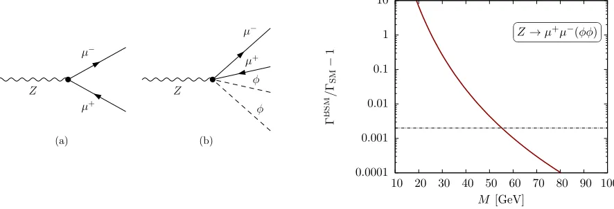
FIG. 2: Modification of the Z boson width to leptons (here concretely forZ →µ+µ−) due to “dressing” the decay using the new interaction with two scalars. The leading order Feynman diagram contributing to this decay is shown in (a) and an example diagram contributing to the modification of the decay at∼1/M4 _{is shown in (b). Note that the individual fermion} legs and the Z boson propagator can also be dressed with a φ2 _{insertion and these diagrams are not shown. Similarly the} production of theZ boson receives modifications. The vertical line represents the current bound onZ→µ+µ−[39].

The size of the BSM correction as a function of M is shown in Fig. 2. We can use this to set a lower limit on M; however an explicit calculation shows that this lower bound is only weak,M &60 GeV.

IV. CONSTRAINTS FROM LHC SEARCHES

The form of the disformal coupling means that disfor-mal scalars can be produced on shell in a collider and, as they will not interact in the detector, will leave only missing energy as a signature of their presence. This means that missing energy searches for dark matter can be adapted to place constraints on disformally coupled dark energy models. In this section we recast recent analyses performed by ATLAS and CMS in the mono-jet [33], mono-photon [34, 35] and di-lepton [36] searches, where available, to reinterpret these measurements and set constraints on the scaleM.† _{By validating our} analy-sis against the 8 TeV results we can also extrapolate our findings to the upcoming run 2 and estimate the limit that will be set in the near future.

For the actual analyses we include the signal and all dominant backgrounds and simulate them with Feyn-Rules [45], MadEvent [46], Sherpa [47] and Her-wig++ [48], jet clustering is performed with Fast-Jet [49]. Throughout the numerical analysis we make the specific choice thatmφ= 1 MeV. However our results will be independent of the mass of such a light scalar, and so will be valid for all lighter masses.

Setting limits on effective field theories at colliders can

†_{Mono-lepton searches [43, 44] crucially depend on a correct} model-ing of the missmodel-ing energy resolution, and we do not consider these searches.

suffer from shortcomings if the new physics scale is re-solved by the experiment [50–55]. An effective field the-ory description is only valid if the probed energy scales are lower than the scale of new physics, e.g. if resonances or thresholds remain unresolved. These shortcomings can be mended by reverting to concrete UV complete sce-narios (but limits become model dependent as a conse-quence) or by separating energy scales consistently on the basis of renormalisation group equations [50, 56]. In the scenario we consider in this paper it is important to high-light a difference compared to similar issues in dark mat-ter searches: while complete field theoretic models can be constructed in dark matter-related analyses, a concrete model implementation is not available in the analysis of strongly coupled gravitational effects due to the intrin-sic non-linear and non-renormalisable nature of gravity in a perturbative field theory context. In what follows, this issue should be kept in mind; while limit setting is a viable qualitative strategy in the absence of a signal, the interpretation of a possible excess seen withM in the TeV region will require the inclusion of non-linear effects which are formally higher order in our (E/M)4 expan-sion. We will comment on the validity of the set limits in light of resolved energy scales later in section V.

Mono-Photon searches

Both ATLAS and CMS have published analyses in mono-photon searches for the full run 1 data set [34, 35] with similar sensitivities.

CMS reconstruct jets using the anti-kT algorithm [57] to cluster particles into jets with resolution parameter‡

450 400 350 300 250 200 150 400

350

300

250

200 observed limit expected limit

Emiss T [GeV]

min

M

[GeV]

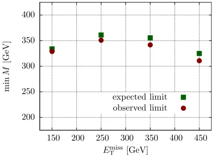
FIG. 3: Results of the ATLAS dilepton search confronted with disformal scalar coupling model. For further details see the text. ATLAS do not quote uncertainties and hence we only show central values.

D= 0.5 and define isolated photons based on the energy deposit in a cone of ∆R =p∆Φ2_{+ ∆η}2 _{< 0.3 (where} Φ and η are the azimuthal angle and pseudo-rapidity, respectively) around the photon candidate, which is re-quired to be smaller than 5% of the candidate’s energy based on the expected shower profile. The transverse en-ergy of the photon is required to beET(γ)>145 GeV. Since a full detector simulation is not available, we ap-proximate this energy with the Monte Carlo information for the transverse momentum. Events with more than one jet with pT > 30 GeV and light leptons (isolation is based on a hadronic energy deposit in the vicinity of ∆R < 0.3 by less than 20% of the candidate pT) with pT >10 GeV are vetoed if they are separated from the photon by ∆R >0.5. The final selection requires a miss-ing transverse energy Emiss

T >140 GeV, well separated from the photon in azimuthal angle ∆Φ(Emiss

T , γ) > 2. We include an expected missing energy resolution by fit-ting the expectation of CMS particle flow as outlined in [59]. After these steps CMS exclude an upper cross sec-tion limit of 14 fb, which translates into a lower limit of

CMS: M &419 GeV (10)

in our analysis.

ATLAS follow a similar strategy, selecting photons withpT(γ)>125 GeV in|ηγ|<1.37, ETmiss>150 GeV and ∆Φ(Emiss

T , γ)>0.4. Jets are reconstructed with the anti-kT algorithm with D = 0.4 and vetoed if pT ,j > 30 GeV and ∆Φ(Emiss

T , j)<0.4. Electrons (pT >7 GeV, |η_| <2.47) and muons (pT >6 GeV, |η| <2.5) are ve-toed. ATLAS exclude 6.1 events at 95% confidence level

to the conical size of the jet combined from particle tracks in the azimuthal angle–pseudo-rapidity plane. An excellent review of jet physics is provided in [58].

for the run 1 luminosity of 20.1/fb. This translates in our implementation into

ATLAS: M &447 GeV, (11)

which is consistent with the CMS limit.

Di-Lepton searches

ATLAS have published a dark matter search in a Z+missing energy search based on the run 1 data set in [36]. In their analysis, ATLAS require electrons to haveET >20 GeV,|η|<2.47 and consider muons with pT > 20 GeV,|η| < 2.5. Isolation is defined by re-quiring the hadronic energy deposit in a cone of size ∆R < 0.2 around the candidate to be less than 10% of the candidate’sET and only tracks withpT >1 GeV are considered in this isolation criterion. Jets are recon-structed with the anti-kT algorithm with D = 0.4, and pT >25 GeV and|η|<2.5.

Candidate events need to have a di-lepton system con-sistent with theZ boson 76 GeV_≤m``≤106 GeV and the missing energy has to be well separated from the di-lepton pair: ∆Φ(Emiss

T , ``) >2.5. Further, ATLAS im-poseη``_<2.5,

|p`` T −E

miss T |/p

``

T <0.5. Events with jets withpT >25 GeV are finally removed and ATLAS con-sider four search regions based on a inclusive selection of missing energy and provide expected and observed fidu-cial cross sections at 95% confidence level.

Implementing these analysis steps, we can again trans-late these limits into lower limits on the disformal cou-pling scale M, as depicted in Fig. 3. The sensitivity is maximised for theEmiss

T >250 GeV search region, where the trade off between differential signal cross section en-hancement due to the probed energy in the disformal cou-pling and decreasing background cross sections becomes optimal. For more stringent requirements, the signal be-comes kinematically suppressed.

Mono-Jet searches

The most recent mono-jet analysis exploiting the full run 1 data set has been provided by the CMS collabora-tion in [33]. In this analysis particles are clustered into jets using the anti-kT algorithm [57] with D = 0.5 and requiring the leading jet to have transverse momentum and rapidity

pT ,j1 >110 GeV,|ηj1|<2.4. (12) A second jet

pT ,j2 >30 GeV,|ηj2|<4.5 (13) is allowed if it is separated from the first jet by

550 500 450 400 350 300 250 1000

750

500

250

observed

expected limit±1σ

CMS extrapolated run 2

CMS, 8 TeV, 19.7/fb

Emiss

T [GeV]

m

in

M

[G

eV

]

FIG. 4: Minimum scaleM extracted from the CMS mono-jet search of [33] in the different search regions based on the inclusive search regions characterised byEmiss

T (for details see text). We also show the improvement based on an extrapo-lation of the 8 TeV analysis to the 13 TeV LHC run 2 with 100/fb.

The analysis vetos events with more than two jets with pT >30 GeV and |ηj|< 4.5. Events with isolated lep-tons are vetoed ifpT ,`>10 GeV; isolation is defined by requiring the total hadronic energy deposit in a cone of size 0.4 around the lepton candidate being smaller than 20% of its transverse momentum. The analysis selects 7 inclusive search regions based on an additional missing energy threshold.

We validate our analysis in these different search re-gions, taking into account theZ+jets, QCD-jets,t¯t+jets, W+ jets and diboson+jets backgrounds and missing en-ergy resolution is included in an analogous manner to that of the previous sections. We find excellent agree-ment of our analysis with the CMS background tem-plates, especially for the dominant backgrounds and most inclusive selections. The agreement of our simulation with the Z + jets template in particular, provides con-fidence that we can set a trustable limit on the presence of an additional missing energy contribution that is the main signature of our model in this channel. For the fake-dominated background contributions as QCD jets, we use the CMS results to derive a differential efficiency, which we will later use in our 13 TeV projections without further modification.

The results of the 8 TeV CMS analysis, recast along the above lines is shown in Fig. 4. Comparing the findings of the mono-jet search to the previously discussed channels, we see that the mono-jet search is the most sensitive to our scenario. In light of this result we extrapolate the 8 TeV CMS to LHC run 2 in Fig. 4 using the CLs method of [60, 61]. Most of this improvement stems from a sig-nificant signal cross section increase by a factor of 10. It is not entirely unexpected that this particular anal-ysis performs better than the other channels discussed above. The particular form of the interaction basically amounts to QCD-like BSM production suppressed by the

H→gg

H→ZZ→4`

H→b¯b

M [GeV]

signal

strength

−

1

220 200 180 160 140 120 100 80 60 10

1

0.1

0.01

FIG. 5: Modifications of the Higgs boson signal strength as a function ofM for the gluon fusion production mode at 8 TeV, estimated using Higgs effective field theory [64–66]. The modifications are analogous to the 2-body and 4-body decay sample Feynman diagrams shown in Fig. 2.

scaleM, and the relative sensitivity follows the paradigm that events induced by strong couplings give tighter con-straints on new physics than those produced by weak couplings because jet production is the most abundant high transverse momentum process at the LHC.

A note on modified Higgs phenomenology

Finally we comment on potential modification of Higgs phenomenology. The crucial observable is the “signal strength”

µik=

[σ{i}(H)×BR(H → {k})]BSM [σ{i}(H)×BR(H→ {k})]SM

, (15)

V. RUNNING OF COUPLINGS

In the previous sections we have focused on direct mea-surements of and constraints on the presence of a mal interaction. In section III A we saw that the disfor-mal scalar does not lead to oblique corrections. Not all BSM effects are expressed through oblique corrections and we analyse other observables in the following. We will see that these effects are highly suppressed and lim-ited to kinematic thresholds in the limit mφ/M 1, where we can trust our expansion in terms of an effective field theory deformation of the SM. We will also comment on potential modifications of the running of couplings due to the presence of the disformal interactions.

Taking the contribution to the vector polarization functions as a starting point we can check whether the presence of the additional derivatively-coupled scalars impacts the running of SM couplings. In particular any impact on the top Yukawa couplings, as well as on the Higgs self interaction will have important consequences on the stability of the electroweak vacuum. By working out the ∼M−4 _{corrections to wave function} renormali-sations and SM vertices we can compute potential con-tributions to the SM β functions. Introducing the MS parameter inD= 4₋2εdimensional regularisation

∆ = Γ(1 +ε) ε

4πµ2 µ2

R

ε

(16)

we haveA0(m2) =m2∆ +O(ε). µR is the renormalisa-tion scale that effectively replacesµ in the renormalisa-tion procedure. We can calculate the renormalisarenormalisa-tion ∼ 1/M4 _{of the Higgs and top wave functions in the} MS scheme (note that all corrections vanish in the limit mφ→0 in dimensional regularisation)

δZH= 1 32π2∆

m_φ

M

4

, (17)

δZt= 3 64π2∆

m_φ

M

4

. (18)

The renormalisation of the ¯ttH vertex to_∼1/M4 _is

δZ¯ttH= 1 16π2 ∆

m_φ

M

4

, (19)

which leads to an operator renormalisation

δZ =δZ¯ttH−δZt− 1

2δZH = 0, (20) which implies no contribution_∼1/M4_{to the anomalous} dimension of the Yukawa coupling yt and its running is therefore not affected by the presence of the disformal coupling.

Similarly we can compute the renormalisation of the quartic interaction operator in the Higgs potential by in-vestigating the four point vertexH4 _{(Fig. 6)}

δZH4= 3 8π2∆

m_φ

M

4

(21)

and again we find an operator renormalisation

δZ =δZH4−2δZ_H= 0, (22) meaning that again the disformal scalar has no impact on the running of the quartic Higgs interaction.

We have checked that similar cancellations happen in the renormalisation of all other SM couplings. This can-cellation is not an accident, but happens due to the inde-pendence of the external and internal symmetries of the considered effective field theory.

The deformation of the disformal interactions, on the other hand, has a dynamic dependence on scale which, if external and internal symmetries are independent, should be limited to the interaction itself as well as invariants of the external (diffeomorphisim) symmetry. Due to the complicated dynamics of the SM as a whole, to analyse this we focus on a simple subsector of the SM; QED with the top as a single massive fermion. Concretely we look at the renormalisation of the operator

Odis= cT M4T

µν_∂

µφ∂νφ (23)

and specifically at the dressed top propagator as probe of the Wilson coefficientcT.

In this model, the wave function renormalisation for the scalarφis given by

δZφ = 21 8π2∆

m_t

M

4

(24)

and the full top renormalisation, including the 1/M0_part in general gauge is

δZt= α 9π∆ξ+

3 64π2∆

m_φ

M

4

, (25)

whereξis the gauge parameter. Theφ2_{-dressed top} prop-agator, Fig. 7 is renormalised by

δZt¯tφ2= α

9π∆ξ (26)

and therefore the operator renormalisation constant is (see e.g. [67] for a detailed discussion of renormali-sation in effective field theories)

δZOdis=− 3 64π2∆

m_φ

M

4

−₈21_π2∆

m_t

M

4

, (27)

which implies an anomalous dimension

γcT =

dδZOdis d logµR

= 1

16π2

3 2

m_φ

M

4

+ 84mt M

4

,

(28)

such that the renormalisation group equation (RGE) reads

cT(Λ) =

Λ M

γcT

H

H

H

H φ

H

H

H

H

φ

φ H

H

H

H

φ φ

H

H

H

H

φ φ

FIG. 6: One-loop corrections to theH4 operator at order 1/M4.

t

t

φ

φ A

t

t

t

t

φ

φ t

A

A

t

t

φ

φ

A t

t

φ

φ t

A

FIG. 7: One-loop corrections to thettφφ¯ vertex in the considered toy model, extended by the disformal coupling.

after inserting the boundary conditioncT(M) = 1. Since the anomalous dimension is positive definite, it flows to small coupling in the infrared, consistent with the behav-ior of a coupling that parametrises the interaction with SM energy-momentum. It is important to note that when calculating the operator renormalisation in Eq. (27) we do not obtain spurious singularities, which would need to be absorbed by additional counter terms unrelated to Odis. The presence of such terms would be tantamount to a RGE flow-induced mixing of _Odis with other inde-pendent operators§ _{that are excluded from our effective} theory of Eq. (23) at the UV scale (by construction). While such terms could in principle be present, see the appendix, our constraints can be understood as consis-tent limits on the operator_Odis alone.

Furthermore, in the previous sections we have found limits in the 650 GeV range, which are mass scales easily resolved by the LHC at 8 TeV. In principle this raises the question of whether we can trust our effective field theory prescription if the most sensitive region to the presence of disformal couplings is given bypT ,j > M in, e.g., the mono-jet analysis. However, equipped with the above RGE equations we can separate the scale of mea-surement and new physics consistently (see e.g. [50] for a related discussion in Higgs phenomenology): If the new physics scale is indeed higher than the resolved scale we can compute the modified limit using RGE equations like Eq. (29). Since the top quark is the heaviest particle in the SM, we can expect that Eq. (29) also gives a reason-able estimate of the size of these effects in the full SM. If we push the fundamental scale M outside the LHC coverage the effectively resolved scale due to Eq. (29) re-mains numerically unchanged due to the smallness of the anomalous dimension γcT and our limit is solid against these aforementioned issues.

§_{Independent in this context means that redundancies are removed} with equations of motion.

The findings for the running of the disformal coupling deserve a few additional remarks. Firstly, the renormal-isation is not only gauge-invariant, i.e. the terms ∼ ξ drop out, but all terms _∼ 1/M0 _{cancel in the} calcula-tion. This means that the internal symmetries which are expressed as the zeroth order in the _∼M−4 _expansion do not influence the running of the disformal coupling. The leading term in the renormalisation only depends on invariants of Lorentz symmetry (masses and gauge cou-plings) and arises purely from wave function renormalisa-tion constants (Eq. (26) is pure gauge), meaning that the coupling remains universal under renormalisation group flow. This is an explicit realisation of the result derived in [68] by Hui and Nicolis, who demonstrated that once a universal coupling between a scalar field and matter has been postulated, this coupling is stable against classical and quantum renormalisations in the matter sector.

If we take the calculation at face value (and neglect the potential presence of higher order terms) the running of cT (with UV boundary conditioncT(M) = 1) is given as a function of all masses in the theory, which displays the running of the energy momentum tensor by all explicit sources of the breaking of conformal invariance.¶ _The running is not influenced by the gauge couplings, this demonstrates that the dynamics of internal and external symmetries factorize reminiscent of the general structure discussed by Coleman and Mandula [70].

VI. CONCLUSIONS

If dark energy couples to matter disformally our best chances to detect these interactions come from events oc-curring at high energies: While precision measurements

at LEP provide a bound onM, the LHC offers the best current prospects for such a study, and we have shown that mono-jet searches performed by the CMS collabo-ration provide the best current constraint on the energy scale of the disformal coupling M &650 GeV. The par-ticular form of the interactions, coupling to the energy momentum tensor, decouples the disformal scalar from precision electroweak observables as well as from the run-ning of SM couplings, in agreement with the expectation of a factorisation of outer and inner symmetries in in-teracting QFT. This leaves direct detection as the main collider avenue to set constraints on the presence of dis-formal couplings. To this end we extrapolate the CMS mono-jet result to the higher energy collisions at the 13 TeV LHC run 2 and estimate that the 8 TeV result can be improved toM &750 GeV for a run 2 luminosity of 100 fb−1, or even higher if systematics are improved.

Acknowledgments

We would like to thank Nemanja Kaloper and David Seery for very helpful discussions during the prepara-tion of this work. PhB acknowledges partial support from the European Union FP7 ITN INVISIBLES (Marie Curie Actions, PITN- GA-2011- 289442) and from the Agence Nationale de la Recherche under contract ANR 2010 BLANC 0413 01. CB is supported by a Royal So-ciety University Research Fellowship. CE is supported in part by the IPPP Associateship programme and is grateful to the Mainz Institute for Theoretical Physics (MITP) for its hospitality and its partial support during the completion of this work.

Appendix: Additional interactions

In this work we have studied the leading order be-haviour when matter fields move on geodesics of a purely

disformal metric. However if we wanted to relax this as-sumption there are a two other possible types of operator that would allow the scalar field to interact with matter in a universal way that have the same mass dimension as those considered here. Firstly, the scalar field may also couple conformally to matter. If this coupling is purely a function of the scalar derivatives then the leading order interaction with matter is:

(β/M4_)(∂φ)2_{T (A.1)}

for constantβ. Secondly, additional terms arise because the energy momentum tensor of the matter fields is only uniquely defined up to addition of terms proportional to the equations of motion. In general relativity the energy momentum tensor remains finite under the renormalisa-tion group flow after allowing for the inclusion of such terms [71]. For the Higgs scalar in Minkowski space, for example, this allows for the inclusion the term

R(˜g)|H|2

(A.2) where ˜gµν is the disformal metric of Eq. (1), and R is the associated Ricci scalar. Written explicitly in terms of the disformal scalar this allows for the inclusion of interactions of the form

γ M4((φ)

2

− ∇µ∇νφ∇µ∇νφ)|H|2 (A.3)

We stress, however, that if β and γ are assumed ini-tially to be zero, as in the main body of this article, then they remain zero under the renormalisation group flow, at least to order (E/M)4_{. If these terms are allowed to} be non-zero then the renormalisation group is expected to mix these coefficients withcT via the equations of mo-tion.

[1] G. Efstathiou, W. Sutherland, and S. Maddox, Nature 348, 705 (1990).

[2] S. Perlmutter et al. (Supernova Cosmology Project), As-trophys.J.517, 565 (1999), astro-ph/9812133.

[3] A. G. Riess et al. (Supernova Search Team), Astron.J. 116, 1009 (1998), astro-ph/9805201.

[4] O. Lahav and A. R. Liddle (2014), 1401.1389. [5] S. Weinberg, Rev.Mod.Phys.61, 1 (1989).

[6] E. J. Copeland, M. Sami, and S. Tsujikawa, Int.J.Mod.Phys.D15, 1753 (2006), hep-th/0603057. [7] T. Clifton, P. G. Ferreira, A. Padilla, and C. Skordis,

Phys.Rept.513, 1 (2012), 1106.2476.

[8] A. Joyce, B. Jain, J. Khoury, and M. Trodden, Phys.Rept.568, 1 (2015), 1407.0059.

[9] E. Adelberger, B. R. Heckel, and A. Nelson, Ann.Rev.Nucl.Part.Sci.53, 77 (2003), hep-ph/0307284.

[10] C. de Rham and A. J. Tolley, JCAP1005, 015 (2010), 1003.5917.

[11] T. Koivisto, D. Wills, and I. Zavala, JCAP1406, 036 (2014), 1312.2597.

[12] J. Alcaraz, J. Cembranos, A. Dobado, and A. L. Maroto, Phys.Rev.D67, 075010 (2003), hep-ph/0212269. [13] J. Cembranos, A. Dobado, and A. L. Maroto, Phys.Rev.

D70, 096001 (2004), hep-ph/0405286.

[14] C. de Rham, G. Gabadadze, and A. J. Tolley, Phys.Rev.Lett.106, 231101 (2011), 1011.1232.

[15] C. de Rham and G. Gabadadze, Phys.Rev.D82, 044020 (2010), 1007.0443.

1407.1861.

[19] J. Sakstein, JCAP1412, 012 (2014), 1409.1734. [20] P. Brax, C. Burrage, and A.-C. Davis, JCAP1210, 016

(2012), 1206.1809.

[21] P. Brax, P. Brun, and D. Wouters (2015), 1505.01020. [22] M. Wyman, Phys.Rev.Lett. 106, 201102 (2011),

1101.1295.

[23] S. Sjors and E. Mortsell, JHEP 1302, 080 (2013), 1111.5961.

[24] M. Zumalacarregui, T. Koivisto, D. Mota, and P. Ruiz-Lapuente, JCAP1005, 038 (2010), 1004.2684.

[25] T. S. Koivisto, D. F. Mota, and M. Zumalacarregui, Phys.Rev.Lett.109, 241102 (2012), 1205.3167.

[26] D. Bettoni, V. Pettorino, S. Liberati, and C. Baccigalupi, JCAP1207, 027 (2012), 1203.5735.

[27] C. van de Bruck, J. Morrice, and S. Vu, Phys.Rev.Lett. 111, 161302 (2013), 1303.1773.

[28] P. Brax, C. Burrage, A.-C. Davis, and G. Gubitosi, JCAP 1311, 001 (2013), 1306.4168.

[29] J. Neveu, V. Ruhlmann-Kleider, P. Astier, M. Besanon, A. Conley, et al., Astron.Astrophys. 569, A90 (2014), 1403.0854.

[30] C. van de Bruck and J. Morrice (2015), 1501.03073. [31] P. Brax, C. Burrage, A.-C. Davis, and G. Gubitosi, JCAP

1503, 028 (2015), 1411.7621.

[32] J. D. Bekenstein, Phys.Rev. D48, 3641 (1993), gr-qc/9211017.

[33] V. Khachatryan et al. (CMS) (2014), 1408.3583. [34] V. Khachatryan et al. (CMS) (2014), 1410.8812. [35] G. Aad et al. (ATLAS), Phys.Rev.D91, 012008 (2015),

1411.1559.

[36] G. Aad et al. (ATLAS), Phys.Rev.D90, 012004 (2014), 1404.0051.

[37] M. E. Peskin and T. Takeuchi, Phys.Rev. D46, 381 (1992).

[38] M. E. Peskin and T. Takeuchi, Phys.Rev.Lett. 65, 964 (1990).

[39] K. Olive et al. (Particle Data Group), Chin.Phys.C38, 090001 (2014).

[40] G. Passarino and M. Veltman, Nucl.Phys. B160, 151 (1979).

[41] A. Denner, Fortsch.Phys.41, 307 (1993), 0709.1075. [42] R. Barbieri, A. Pomarol, R. Rattazzi, and A. Strumia,

Nucl.Phys.B703, 127 (2004), hep-ph/0405040. [43] V. Khachatryan et al. (CMS) (2014), 1408.2745. [44] G. Aad et al. (ATLAS), Phys.Rev.D90, 012004 (2014),

1404.0051.

[45] A. Alloul, N. D. Christensen, C. Degrande, C. Duhr, and B. Fuks, Comput.Phys.Commun.185, 2250 (2014),

1310.1921.

[46] J. Alwall, M. Herquet, F. Maltoni, O. Mattelaer, and T. Stelzer, JHEP1106, 128 (2011), 1106.0522.

[47] T. Gleisberg, S. Hoeche, F. Krauss, M. Schonherr, S. Schumann, et al., JHEP0902, 007 (2009), 0811.4622. [48] M. Bahr, S. Gieseke, M. Gigg, D. Grellscheid, K.

Hamil-ton, et al., Eur.Phys.J.C58, 639 (2008), 0803.0883. [49] M. Cacciari, G. P. Salam, and G. Soyez, Eur.Phys.J.

C72, 1896 (2012), 1111.6097.

[50] C. Englert and M. Spannowsky, Phys.Lett. B740, 8 (2015), 1408.5147.

[51] O. Buchmueller, M. J. Dolan, and C. McCabe, JHEP 1401, 025 (2014), 1308.6799.

[52] P. Harris, V. V. Khoze, M. Spannowsky, and C. Williams, Phys.Rev.D91, 055009 (2015), 1411.0535.

[53] T. Jacques and K. Nordstrm (2015), 1502.05721. [54] M. R. Buckley, D. Feld, and D. Goncalves, Phys.Rev.

D91, 015017 (2015), 1410.6497.

[55] U. Haisch and E. Re (2015), 1503.00691.

[56] G. Isidori, A. V. Manohar, and M. Trott, Phys.Lett. B728, 131 (2014), 1305.0663.

[57] M. Cacciari, G. P. Salam, and G. Soyez, JHEP0804, 063 (2008), 0802.1189.

[58] G. P. Salam, Eur.Phys.J.C67, 637 (2010), 0906.1833. [59] C. Englert, M. Spannowsky, and C. Wymant, Phys.Lett.

B718, 538 (2012), 1209.0494.

[60] A. L. Read, J.Phys.G28, 2693 (2002). [61] A. L. Read, CERN-OPEN-2000-205 (2000).

[62] C. Englert, A. Freitas, M. Mhlleitner, T. Plehn, M. Rauch, et al., J.Phys.G41, 113001 (2014), 1403.7191. [63] M. Klute, R. Lafaye, T. Plehn, M. Rauch, and D. Zerwas,

Europhys.Lett.101, 51001 (2013), 1301.1322.

[64] B. A. Kniehl and M. Spira, Z.Phys.C69, 77 (1995), hep-ph/9505225.

[65] J. R. Ellis, M. K. Gaillard, and D. V. Nanopoulos, Nucl.Phys.B106, 292 (1976).

[66] M. A. Shifman, A. Vainshtein, M. Voloshin, and V. I. Zakharov, Sov.J.Nucl.Phys.30, 711 (1979).

[67] G. Buchalla, A. J. Buras, and M. E. Lautenbacher, Rev.Mod.Phys.68, 1125 (1996), hep-ph/9512380. [68] L. Hui and A. Nicolis, Phys.Rev.Lett. 105, 231101

(2010), 1009.2520.

[69] C. Englert, J. Jaeckel, V. Khoze, and M. Spannowsky, JHEP1304, 060 (2013), 1301.4224.

[70] S. R. Coleman and J. Mandula, Phys.Rev. 159, 1251 (1967).