Mod´elisation Math´ematique et Analyse Num´erique
hp
–VERSION DISCONTINUOUS GALERKIN METHODS FOR
ADVECTION–DIFFUSION–REACTION PROBLEMS ON POLYTOPIC MESHES
ANDREA CANGIANI
1, ZHAONAN DONG
1, EMMANUIL H. GEORGOULIS
2and PAUL HOUSTON
3Abstract. We consider thehp–version interior penalty discontinuous Galerkin finite element method (DGFEM) for the numerical approximation of the advection–diffusion–reaction equation on general computational meshes consisting of polygonal/polyhedral (polytopic) elements. In particular, newhp– versiona priorierror bounds are derived based on a specific choice of the interior penalty parameter which allows for edge/face–degeneration. The proposed method employs elemental polynomial bases of total degreep(Pp–basis) defined in the physical coordinate system, without requiring the mapping
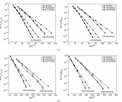
from a given reference or canonical frame. Numerical experiments highlighting the performance of the proposed DGFEM are presented. In particular, we study the competitiveness of the p–version DGFEM employing a Pp–basis on both polytopic and tensor–product elements with a (standard)
DGFEM employing a (mapped)Qp–basis. Moreover, a computational example is also presented which
demonstrates the performance of the proposedhp–version DGFEM on general agglomerated meshes. R´esum´e. ...
1991 Mathematics Subject Classification. 65N30, 65N50, 65N55. ...
1.
Introduction
Discontinuous Galerkin methods have enjoyed considerable success, especially during the last 15 years and are now considered a standard variational framework for the numerical solution of many classes of problems involving partial differential equations (PDEs). The origins of the discontinuous Galerkin finite element method (DGFEM, for short) can be traced back to the early 1970s for the numerical solution of first–order hyperbolic problems [45] and for the weak imposition of inhomogeneous boundary conditions for elliptic problems [42]. The use of discontinuous/nonconforming approximation spaces in the context of finite element methods also
Keywords and phrases: discontinuous Galerkin; polygonal elements; polyhedral elements; hp–finite element methods; inverse estimates;P–basis; PDEs with nonnegative characteristic form.
1 Department of Mathematics, University of Leicester, Leicester LE1 7RH, UK;
e-mail: [email protected]; [email protected]
2 Department of Mathematics, University of Leicester, Leicester LE1 7RH, UK
& School of Applied Mathematical and Physical Sciences, National Technical University of Athens, Athens 15780, Greece; e-mail: [email protected]
3 School of Mathematical Sciences, University of Nottingham, Nottingham, NG7 2RD, UK;
e-mail: [email protected]
c
first appeared around the same time [12, 13]; for reviews of some of the main developments in the subject, we refer to the monographs [27, 28] and the articles [8, 24].
The interest in DGFEMs can be attributed to a number of factors: classical DGFEMs, such as interior penalty methods, have typically minimal communication, in the sense that only direct face-element neigh-bours are coupled through the exploitation of appropriate numerical fluxes; this has important advantages for imposing boundary conditions and also for parallel efficiency. Additionally, DGFEMs can incorporate a wealth of numerical fluxes into their formulation, leading to stable discretizations in the context of multi-scale problems. Moreover, meshes containing hanging-nodes and elemental polynomial bases consisting of locally variable polynomial degrees are also admissible, owing to the lack of pointwise continuity requirements across the mesh-skeleton. Also, powerful solvers are now available for the resulting linear systems; indeed, both domain decomposition preconditioners, see, for example, [1, 2, 4, 5, 29, 39], and the references cited therein, as well as multigrid solvers, cf. [6, 7, 17, 18], have been developed.
More recently, DGFEMs on meshes containing extremely general element shapes, such as general polygons in two dimensions and polyhedra in three dimensions, have been proposed [3, 14–16, 21, 28, 33, 40, 50]. Such meshes can naturally be combined with DGFEMs due to their element-wise discontinuous approximation. To support such a variety of element shapes, without any detrimental affect on the local approximation properties of the underlying DGFEM, polynomial spaces defined in the physical frame, rather than mapped polynomials from a reference element, are typically employed. In our recent work [21], an hp–version DGFEM of interior penalty (IP) type for linear elliptic problems on meshes consisting of d–dimensional polytopic elements (i.e., polygons ford= 2 and polyhedra ford= 3) was proposed and analysed. A key aspect of the method proposed in [21], is that the scheme remains well-defined and practical in the presence of arbitrarily small/degenerate (d−k)–dimensional element facets,k= 1, . . . , d−1, where ddenotes the spatial dimension. A by-product of the approach developed in [21] was the proposal of physical framePp–type bases, i.e., local polynomial spaces of
total degreep, for the case when the underlying polytopes are simply quadrilateral/hexahedral, compared to the standard approach of employing a mapped tensor-productQppolynomial basis, i.e., tensor-product polynomials of degree p in each spatial variable. Indeed, it was demonstrated numerically that the DGFEM employing a Pp–type basis achieves a faster rate of convergence, with respect to the number of degrees of freedom present in the underlying finite element space, as the polynomial degree pincreases, for a given fixed mesh, than the respective DGFEM employing a (mapped)Qp basis on tensor-product elements.
In this work, we extend the results of [21] to cover hp–version IP DGFEMs for a general class of linear advection–diffusion–reaction PDE problems, often referred to as equations with nonnegative characteristic form. DGFEMs for this class of problems on quadrilateral meshes were first proposed and analysed in [35]. Here, we derive a priori bounds for the hp–version IP DGFEM for this class of PDE problems. Due to the lack of hp–approximation results for the local L2–projection operator on polytopic elements, it is not possible to directly generalise the analysis from [35] to meshes consisting of such elements. To address this issue, we prove an inf-sup condition for the underlying DGFEM, with respect to a stronger streamline–diffusion type norm, for simple advection coefficients, thereby extending respective results from [9, 19, 20, 37] to the current setting. This naturally leads toa prioribounds for thehp–version DGFEM for this general class of linear PDE problems on very general polytopic meshes with possibly arbitrarily small/degenerate (d−k)–dimensional element facets,
k= 1, . . . , d−1.
2.
Preliminaries
For a Lipschitz domain ω⊂Rd, d≥1, we denote byHs(ω) the Hilbertian Sobolev space of indexs≥0 of real–valued functions defined on ω, endowed with the seminorm | · |Hs(ω) and norm ∥ · ∥Hs(ω). Furthermore,
we letLp(ω),p∈[1,∞], be the standard Lebesgue space onω, equipped with the norm∥ · ∥Lp(ω). Finally,|ω|
denotes thed–dimensional Hausdorff measure ofω.
2.1.
Model problem
Let Ω be a bounded open polyhedral domain in Rd, d = 2,3, and let Γ signify the union of its (d−1)– dimensional open faces. We consider the advection-diffusion-reaction equation
Lu≡ −∇ ·(a∇u) +b· ∇u+cu=f, in Ω, (2.1)
where c ∈ L∞(Ω), f ∈ L2(Ω), and b := (b1, b2, . . . , bd)⊤ ∈ [W∞1(Ω)]d. Here, a = {aij}di,j=1 is a symmetric positive semidefinite tensor whose entriesaij are bounded, piecewise continuous, real-valued functions defined on ¯Ω, with
ξ⊤a(x)ξ≥0 ∀ξ∈Rd, a.e. x∈Ω¯. (2.2) Under the above hypothesis, (2.1) is termeda partial differential equation with nonnegative characteristic form. We denote by n(x) ={ni(x)}di=1 the unit outward normal vector to Γ at x∈ Γ and introduce the Fichera functionb·nto define
Γ0=
{
x∈Γ :n(x)⊤a(x)n(x)>0
} ,
Γ−=
{
x∈Γ\Γ0:b(x)·n(x)<0
}
, Γ+=
{
x∈Γ\Γ0:b(x)·n(x)≥0
} .
(2.3)
The sets Γ−and Γ+are referred to as the inflow and outflow boundary, respectively. Note that Γ = Γ0∪Γ−∪Γ+. If Γ0 is nonempty, we subdivide it into two disjoint subsets ΓD and ΓN whose union is Γ0, with ΓD nonempty and relatively open in Γ, on which we consider the boundary conditions for (2.1):
u=gD on ΓD∪Γ−, n·(a∇u) =gN on ΓN, (2.4) and also adopt the hypothesis that b·n≥0 on ΓN, whenever ΓN is nonempty. Additionally, we assume that the following positivity hypothesis holds: there exists a positive constant γ0 such that
c0(x)2:=c(x)− 1
2∇ ·b(x)≥γ0 a.e. x∈Ω. (2.5) The well-posedness of the boundary value problem (2.1), (2.4) has been studied in [36].
2.2.
Finite element spaces
other, while in three–dimensions this may no longer be the case, since the boundary of a general polyhedron may consist of planar polygons which are not triangular.
As in [21], we assume that a sub-triangulation into faces of each mesh interface is given ifd= 3, and denote by E the union of all open mesh interfaces ifd= 2 and the union of all open triangles belonging to the sub-triangulation of all mesh interfaces if d= 3. In this way, E is always defined as a set of (d−1)–dimensional simplices. Further, we writeEint to denote the union of all open (d−1)–dimensional element faces F ⊂ E that are contained in Ω, and let Γint :={x∈Ω :x∈F, F ∈ Eint}. Further assumptions on the class of admissible meshes will be outlined later on in Section 4.
Given κ∈ T, we writepκ to denote the (positive)polynomial degree of the elementκ, and collect thepκ in the vectorp:= (pκ:κ∈ T). We then define thefinite element space STp with respect toT andpby
STp:={u∈L2(Ω) :u|κ∈ Ppκ(κ), κ∈ T },
where Ppκ(κ) denotes the space of polynomials of total degree pκ on κ. As in [21], we point out that the
local elemental polynomial spaces employed within the definition of STp are defined in the physical coordinate system, without the need to map from a given reference or canonical frame. We define the broken Sobolev space
Hs(Ω,T) with respect to the subdivisionT up to composite ordersas follows
Hs(Ω,T) ={u∈L2(Ω) :u|κ∈Hsκ(κ) ∀κ∈ T }. (2.6)
For u ∈ H1(Ω,T), we define the broken gradient ∇hu by (∇hu)|κ = ∇(u|κ), κ ∈ T, which will be used to construct the forthcoming DGFEM.
2.3.
Trace operators
For any elementκ∈ T, we denote by∂κthe union of (d−1)–dimensional open faces ofκ. Then, the inflow and outflow parts of∂κ are defined as follows
∂−κ={x∈∂κ, b(x)·nκ(x)<0}, ∂+κ={x∈∂κ, b(x)·nκ(x)≥0},
respectively, where nκ(x) denotes the unit outward normal vector to ∂κ at x∈ ∂κ. Givenκ ∈ T, the trace of a function v ∈H1(Ω,T) on ∂−κ, relative to κ, is denoted by v+κ. Further, if∂−κ\Γ is nonempty, then for
x∈∂−κ\Γ there exits a unique κ′ ∈ T such thatx∈∂+κ′; with this notation, we denote byv−κ the trace of
v|κ′ on ∂−κ\Γ. Hence theupwind jump of the (scalar-valued) functionv across a faceF ⊂∂−κ\Γ is denoted by
⌊v⌋:=vκ+−vκ−.
Next, we introduce some additional trace operators. Letκi andκj be two adjacent elements ofT and letx be an arbitrary point on the interior faceF ⊂Γint given byF =∂κi∩∂κj. We writeni andnj to denote the outward unit normal vectors onF, relative to∂κiand∂κj, respectively. Furthermore, letvandqbe scalar- and vector-valued functions, which are smooth inside each elementκi and κj. By (vi,qi) and (vj,qj), we denote the traces of (v,q) on F taken from within the interior ofκi and κj, respectively. The averages of v andq at
x∈F are given by
{{v}}:=1
2(vi+vj), {{q}}:= 1
2(qi+qj), respectively. Similarly, the jump ofv andqatx∈F ⊂Γint are given by
[[v]] :=vini+vjnj, [[q]] :=qi·ni+qj·nj, respectively. On a boundary faceF ⊂Γ, such thatF ⊂∂κi,κi∈ T, we set
withni denoting the unit outward normal vector on the boundary Γ.
Remark 2.1. The jump operator [[·]] is independent of face orientation, while the sign of the upwind jump operator ⌊·⌋ depends on the direction of the flow.
3.
Interior Penalty Discontinuous Galerkin Method
In this section, we introduce thehp–version DGFEM discretization of the model problem (2.1), (2.4). For simplicity of presentation, we suppose that the entries of the diffusion tensora are constant on each element
κ∈ T, i.e.,
a∈[ST0]dsym×d. (3.1)
Our results can easily be extended to the case of general a ∈ L∞(Ω)d×d
sym based on employing the modified DGFEM proposed in [32]. In the following,√adenotes the (positive semidefinite) square-root of the symmetric matrixa; further, ¯aκ:=|
√ a|2
2|κ, where | · |2denotes thel2–norm. The IP DGFEM is given by: finduh∈S
p
T such that
B(uh, vh) =ℓ(vh) (3.2)
for allvh∈S
p
T. Here, the bilinear form B(·,·) :STp×STp→Ris defined as the sum of two parts:
B(u, v) :=Bar(u, v) +Bd(u, v),
where the bilinear formBar(·,·) accounts for the advection and reaction terms:
Bar(u, v) :=
∑
κ∈T
∫
κ
(
b· ∇u+cu )
vdx
−∑
κ∈T
∫
∂−κ\Γ
(b·n)⌊u⌋v+ds−∑
κ∈T
∫
∂−κ∩(ΓD∪Γ−)
(b·n)u+v+ds. (3.3)
The bilinear formBd(·,·) takes care of the diffusion term:
Bd(u, v) :=
∑
κ∈T
∫
κ
a∇u· ∇vdx+
∫
Γint∪ΓD
σ[[u]]·[[v]] ds
− ∫
Γint∪ΓD (
{{a∇hu}} ·[[v]] +{{a∇hv}} ·[[u]]
)
ds. (3.4)
Furthermore, the linear functionalℓ:STp →Ris defined by
ℓ(v) := ∑ κ∈T
∫
κ
f vdx−∑
κ∈T
∫
∂−κ∩(ΓD∪Γ−)
(b·n)gDv+ds
− ∫
ΓD gD
(
(a∇hv)·n−σv
)
ds+
∫
ΓN
gNvds. (3.5)
The nonnegative function σ∈ L∞(Γint∪ΓD) appearing in (3.4) and (3.5) is referred to as the
discontinuity-penalization parameter; its precise definition, which depends on the diffusion tensor a and the discretization
4.
Approximation and Inverse Estimates
In this section, we revisit some polynomial approximation and inverse estimates in the context of general polytopic elements from [21]. Furthermore, we derive a new extension of a standard inverse estimate for polynomial functions. To this end, we introduce the following set of mesh assumptions.
Assumption 4.1. The subdivisionT is shape regular in the sense of [23], i.e., there exists a positive constant
Cshape, independent of the mesh parameters, such that:
∀κ∈ T, hκ
ρκ
≤Cshape,
with ρκ denoting the diameter of the largest ball contained in κ.
Assumption 4.2. There exists a positive constantCF, independent of the mesh parameters, such that max
κ∈T (card{F ⊂Γ∪Γint :F ⊂∂κ})≤CF.
Remark 4.1. We note that Assumption 4.2 naturally imposes the condition that the number of hanging nodes
and the number of faces that each elementκin the finite element meshT possesses is uniformly bounded under
mesh refinement.
As in [21], we require the existence of the following coverings of the mesh.
Definition 4.1. A (typically overlapping) coveringT♯={K}related to the polytopic meshT is a set of
shape-regular d–simplicesK, such that for eachκ∈ T, there exists aK ∈ T♯, withκ⊂ K. Given T♯, we denote by Ω♯
the covering domaingiven byΩ♯:=(∪K∈T♯K¯)◦, where, for a closed setD⊂Rd,D◦ denotes the interior ofD.
Assumption 4.3. There exists a covering T♯ of T and a positive constant OΩ, independent of the mesh
parameters, such that the subdivisionT satisfies
max
κ∈T Oκ≤ OΩ,
where, for eachκ∈ T,
Oκ:=card{κ′ ∈ T :κ′∩ K ̸=∅, K ∈ T♯ such that κ⊂ K}.
As a consequence, we deduce that
diam(K)≤Cdiamhκ,
for each pairκ∈ T,K ∈ T♯, withκ⊂ K, for a constant Cdiam>0, uniformly with respect to the mesh size.
We remark that Assumption 4.3 ensures that the amount of overlap present in the covering T♯ remains bounded as the computational mesh T is refined. The proceeding hp–approximation results and inverse esti-mates for polytopic elements are based on referring back tod–dimensional simplices, where standard results can be applied; see, for example, [10, 11, 22, 41]. With this in mind, we introduce the following definition.
Definition 4.2. For each element κ in the computational mesh T, we define the family F♭κ of all possible
d–dimensional simplices contained in κand having at least one face in common with κ. The notation κF
♭ will
be used to indicate a simplex belonging toFκ
♭ and sharing withκ∈ T a given face F.
Theorem 4.1. Let Ω be a domain with a Lipschitz boundary. Then there exists a linear extension operator
E:Hs(Ω)→Hs(Rd),s∈N
0, such that Ev|Ω=v and
∥Ev∥Hs(Rd)≤C∥v∥Hs(Ω),
whereC is a positive constant depending only on s andΩ.
With the above notation, we now quote Lemma 4.2 from [21].
Lemma 4.1. Let κ∈ T,F ⊂∂κ denote one of its faces, and K ∈ T♯ denote the corresponding simplex such
that κ⊂ K, cf. Definition 4.1. Suppose that v ∈L2(Ω) is such that Ev|K ∈Hlκ(K), for some lκ ≥0. Then,
given Assumption 4.3 is satisfied, there existsΠ˜v, such that Π˜v|κ∈ Ppκ(κ), and the following bounds hold
∥v−Π˜v∥Hq(κ)≤C
hsκ−q
κ
plκ−q
κ
∥Ev∥Hlκ(K), lκ≥0, (4.1)
for0≤q≤lκ, and
∥v−Π˜v∥L2(F)≤C|F|
1/2h sκ−d/2
κ
plκ−1/2
κ
Cm(pκ, κ, F)1/2∥Ev∥Hlκ(K), lκ> d/2, (4.2)
where
Cm(pκ, κ, F) = min
{
hdκ
supκF ♭⊂κ|κ
F ♭|
, 1 p1κ−d
} .
Here, sκ = min{pκ+ 1, lκ} and C is a positive constant, that depends on the shape-regularity of K, but is
independent of v,hκ, andpκ.
We now consider the derivation of hp–version inverse estimates, which are sharp with respect to (d−k)– dimensional, k= 1, . . . , d−1, element facet degeneration. To this end, we first recall the following definition, cf. [21].
Definition 4.3. LetT˜ denote the subset of elements κ,κ∈ T, such that eachκ∈T˜ can be covered by at most
mT shape-regular simplicesKi,i= 1, . . . , mT, such that
dist(κ, ∂Ki)> Casdiam(Ki)/p2κ,
and
|Ki| ≥cas|κ|
for all i = 1, . . . , mT, for some mT ∈ N and Cas, cas > 0, independent of κ and T, where pκ denotes the
polynomial degree associated with element κ,κ∈ T.
The motivation for Definition 4.3 comes from the following result, which is derived in [31] and is instrumental in proving the inverse estimate stated in Lemma 4.3 below.
Lemma 4.2. Let K be a shape-regular simplex. For each v ∈ Pp(K), there exists a simplex κˆ ⊂K, having
the same shape as K and faces parallel to the faces ofK, withdist(∂κ, ∂Kˆ )> Casdiam(K)/p2(>0), for some
constant Cas>0, independent ofv,K andp, such that
∥v∥L2(ˆκ)≥
1
2∥v∥L2(K).
Lemma 4.3. Letκ∈ T,F ⊂∂κdenote one of its faces, andT˜ be defined as in Definition 4.3. Then, for each
v∈ Pp(κ), we have the inverse estimate
∥v∥2L
2(F)≤CINV(p, κ, F) p2|F|
|κ| ∥v∥
2
L2(κ), (4.3)
where
CINV(p, κ, F) :=Cinv
min
{
|κ|
supκF ♭⊂κ|κ
F ♭|
, p2d }
, ifκ∈T˜,
|κ|
supκF ♭⊂κ|κ
F ♭|
, ifκ∈ T \T˜,
and κF
♭ ∈ F κ
♭ is as in Definition 4.2. Furthermore, Cinv is a positive constant, which, if κ ∈T˜, depends on
the shape regularity of the covering of κgiven in Definition 4.3, but is always independent of|κ|/supκF ♭⊂κ|κ
F ♭|
(and, therefore, of |F|),p, andv.
The following assumption plays a key role in deriving the extension of the standard inverse estimate for the
H1-(semi)norm.
Assumption 4.4. Every polytopic element κ∈ T \T˜, admits a sub-triangulation into at mostnT shape-regular simplices si,i= 1,2, . . . , nT, such that ¯κ=∪ni=1T ¯si and
|si| ≥ˆc|κ|
for alli= 1, . . . , nT, for somenT ∈Nandˆc >0, independent ofκandT.
Lemma 4.4. Given Assumptions 4.1-4.4 are satisfied, for each v∈ Pp(κ), the inverse estimate
∥∇v∥2L
2(κ)≤ ˜
Cinv
p4
h2 κ
∥v∥2L
2(κ), (4.4)
holds, with constantC˜inv independent of the element diameterhκ, the polynomial order pκ, and the functionv,
but dependent on the shape regularity of the covering ofκ, ifκ∈T˜, or the sub-triangulation ofκ, ifκ∈ T \T˜.
Proof. Here, we only consider the case whenκ∈T˜; for κ∈ T \T˜ the inverse inequality follows in a straight-forward manner by exploiting the sub-triangulation introduced in Assumption 4.4, together with the standard inverse estimate applied to each sub-simplex. Givenκ∈T˜, we have a covering ofκby shape-regular simplices
Kj,j = 1, . . . , mT, with|Kj| ≥cas|κ|, cf. Definition 4.3. The shape-regularity Assumption 4.1, in conjunction with the trivial relationhdκ≥ |κ| ≥ρdκ, yields
hdKj ≥ |Kj| ≥cas|κ| ≥casρdκ≥cas
( hκ
Cshape
)d
, (4.5)
where hKj denotes the diameter of Kj. Hence, hKj ≥ (cas)
1/dh
κ/Cshape. The standard inverse inequality applied onKj yields
∥∇v∥L2(Kj)≤C2
p2 hKj
where the positive constant C2 is independent of p, hKj, and v; see [46] for details. Employing (4.6) and
Definition 4.3 again, we deduce that
∥∇v∥2L
2(κ) ≤ mT
∑
j=1
∥∇v∥2L
2(Kj)
≤ C2
mT
∑
j=1
p4 h2
Kj
∥v∥2L
2(Kj)
≤ C2C
2 shape (cas)2/d
p4 h2 κ
mT
∑
j=1
∥v∥2L
2(Kj). (4.7)
Let ˆκj ⊂Kj denote the simplex given by Lemma 4.2; then by the same Lemma 4.2 and Definition 4.3, we have
1 4∥v∥
2
L2(Kj)≤ ∥v∥
2
L2(ˆκj)≤ ∥v∥
2
L2(Kj∩κ), (4.8)
since ˆκj ⊂κ, and hence ˆκj⊂Kj∩κ⊂Kj, cf. [21]. Combining (4.7) and (4.8), we deduce that
∥∇v∥2L
2(κ)≤
4C2Cshape2 mT (cas)2/d
p4 h2 κ
∥v∥2L
2(κ)≡ ˜
Cinv
p4 h2 κ
∥v∥2L
2(κ), (4.9)
as required. □
Remark 4.2. We point out that Assumption 4.1, which imposes the shape regularity of the mesh T, is only
needed for the proof of Lemma 4.4; this result extends the classical inverse estimate, bounding theH1-seminorm
of a polynomial function with itsL2-norm, to polytopic elements. We note, however, that such inverse estimates
depend on the shape regularity of the elements, even in the case of simplicial elements, cf. [49]. An alternative
hp–version inverse inequality, analogous to Lemma 4.4, with explicit dependence on the shape-regularity, is
derived in [6].
5.
A priori error bound for the DGFEM
Thea priori error analysis will employ an inconsistent formulation of the diffusion part of the bilinear form, cf. [43], for example. We define, for allu, v∈ S:=H1(Ω) +Sp
T, the bilinear form
˜
B(u, v) :=Bar(u, v) + ˜Bd(u, v), (5.1)
where
˜
Bd(u, v) :=
∑
κ∈T
∫
κ
a∇u· ∇vdx+
∫
Γint∪ΓD
σ[[u]]·[[v]] ds
− ∫
Γint∪ΓD (
{{aΠ2(∇hu)}} ·[[v]] +{{aΠ2(∇hv)}} ·[[u]]
)
ds,
and the linear functional ˜ℓ:SpT →Rby
˜
ℓ(v) := ∑ κ∈T
∫
κ
f vdx−∑
κ∈T
∫
∂−κ∩(ΓD∪Γ−)
(b·n)gDv+ds
− ∫
ΓD gD
(
aΠ2(∇hv)·n−σv
)
ds+
∫
ΓN
Here, Π2 : [L2(Ω)]d → [S
p−1
T ]d denotes the L2–projection onto the finite element space [S
p−1
T ]d. We then
rewrite the discrete problem with the inconsistent formulation in the equivalent form: finduh∈S
p
T such that
˜
B(uh, vh) = ˜l(vh) ∀vh∈STp. (5.2)
In view of the error analysis, we introduce the DGFEM-norm|∥·|∥DG as the sum of two parts as follows:
|∥v|∥2DG:=|∥v|∥2ar+|∥v|∥2d,
where
|∥v|∥2ar :=
∑
κ∈T
(
∥c0v∥2L2(κ)+
1 2∥v
+∥2
∂−κ∩(ΓD∪Γ−)+ 1 2∥v
+−
v−∥2∂−κ\Γ+1 2∥v
+∥2 ∂+κ∩Γ
)
, (5.3)
withc0as in (2.5), and
|∥v|∥2d:= ∑
κ∈T
∥√a∇v∥2L
2(κ)+ ∫
Γint∪ΓD
σ|[[v]]|2ds. (5.4)
Here, ∥ · ∥τ,τ⊂∂κ, denotes the (semi)norm associated with the (semi)inner product (v, w)τ =
∫
τ|b·n|vwds. The following relation holds
Bar(v, v) =|∥v|∥2ar (5.5)
for all v ∈ S, cf. [35]. The continuity and coercivity of the inconsistent diffusion bilinear form ˜Bd(·,·), with respect to the DGFEM-norm|∥·|∥d, is established by the following lemma.
Lemma 5.1. Let σ: Γ\ΓN→R+ be defined facewise by
σ(x) :=
Cσ max κ∈{κ1,κ2}
{
CINV(pκ, κ, F) ¯
aκp2κ|F|
|κ|
}
, x∈F ⊂Γint, F =∂κ1∩∂κ2,
CσCINV(pκ, κ, F) ¯
aκp2κ|F|
|κ| , x∈F ⊂ΓD, F =∂κ∩ΓD,
(5.6)
with Cσ >0 large enough, and independent of pκ, |F|, and|κ|; here CINV is defined as in Lemma 4.3. Then,
given Assumption 4.2 holds, we have that
˜
Bd(v, v)≥Cdcoer|∥v|∥ 2
d for all v∈ S, (5.7)
and
˜
Bd(w, v)≤Cdcont|∥w|∥d|∥v|∥d for all w, v∈ S, (5.8)
whereCcont d andC
coer
d are positive constants independent of the discretization parameters.
Proof. The proof can be viewed as an extension of the analogous result derived in [21] for the Poisson equation, to a second–order elliptic PDE with general positive semidefinite diffusion tensora; for details, we refer to [32]. □
5.1.
Inf-Sup Condition
Definition 5.1. The streamline DGFEM-norm is defined by:
|∥v|∥2s:=|∥v|∥2DG+
∑
κ∈T
τκ∥b· ∇v∥2L2(κ), (5.9)
where
τκ:= min
{
1
∥b∥L∞(κ)
, 1
˜
σκ
} h⊥κ p2 κ
∀κ∈ T, (5.10)
forpκ≥1, and˜σκ is given by
˜
σκ := Cσ max F⊂∂κ
{
max ˜ κ∈{κ,κ′} F⊂∂κ∩∂κ′
{ Cinv
¯
a˜κp2κ˜
h⊥˜κ d }}
∀κ⊂ T, d= 2,3, (5.11)
where Cinv is defined as in Lemma 4.3. The constantσ˜κ may be zero locally where ¯aκ = 0; in this case it is
understood that τκ takes the value of the first term in (5.10). Further, the mesh parameter h⊥κ is defined as
follows:
h⊥κ := min F⊂∂κ
supκF ♭⊂κ|κ
F ♭|
|F| d ∀κ∈ T, d= 2,3, (5.12)
with κF
♭ as in Definition 4.2. We further deduce the relation
h⊥κ ≤hκ. (5.13)
Remark 5.1. We recall from Definition 4.2 thatκF
♭ denotes the family of simplices contained inκand sharing
a face F with κ. From the geometrical property of d–dimensional simplices, it is easy to see that h⊥κ is the minimum over all faces F,F ⊂∂κ, of the maximum of the set of all heights of thed–dimensional simplicesκF ♭
sharing a(d−1)–dimensional face F withκ.
Remark 5.2. With a mild loss of generality, the casepκ= 0, relevant to the hyperbolic regime, is excluded from
Definition 5.1 and throughout this paper. However, if the underlying problem is strictly hyperbolic and pκ= 0
is selected for all κ∈ T, then the streamline DGFEM-norm reduces to the advection-reaction DGFEM-norm
|∥·|∥ar defined in (5.3); in this setting, the proceeding analysis is trivial.
By employing the definition of h⊥κ, together with an upper bound on the constant CINV(p, κ, F) defined in Lemma 4.3, the inverse estimate (4.3) can be written in the following manner. For eachv∈ Pp(κ),F ⊂∂κ, we have
∥v∥2L
2(F) ≤ CINV(p, κ, F) p2|F|
|κ| ∥v∥
2 L2(κ)
≤ Cinv |
κ|
supκF ♭⊂κ|κ
F ♭|
p2|F|
|κ| ∥v∥
2
L2(κ)≤Cinv p2
h⊥κd∥v∥
2
L2(κ). (5.14)
Further, from the definition ofσ|F given in (5.6), in conjunction with the definition ofh⊥κ, cf. (5.12), we deduce the following bound
˜
σκ ≥ σ|F, F ⊂∂κ∀κ∈ T. (5.15)
For the reminder of this article we assume the following standard condition onb: b· ∇hξ∈S
p
T ∀ξ∈STp, (5.16)
Theorem 5.1. Given Assumptions 4.1, 4.2, and 4.4 hold, there exists a positive constant Λs, independent of
the mesh sizehand the polynomial degree p, such that:
inf ν∈STp\{0}
sup µ∈STp\{0}
˜
B(ν, µ)
|∥ν|∥s|∥µ|∥s
≥Λs, (5.17)
where the discontinuity-penalization parameter σis as defined in (5.6).
Proof. For allν ∈STp, we selectµ:=ν+ανs,νs|κ=τκb· ∇ν for allκ∈ T, whereαis a positive real number, chosen sufficiently small, cf. (5.32) below. By (5.16), we note thatµ∈STp; the theorem now follows from the two bounds:
|∥µ|∥s≤C∗|∥ν|∥s, (5.18) and
˜
B(ν, µ)≥C∗|∥ν|∥2s, (5.19) with Λs=C∗/C∗, whereC∗and C∗ are positive constants, independent ofhandp.
We begin by proving (5.18). We first bound each term arising in the norm|∥·|∥arofνs, whereνs|κ=τκb·∇ν,
κ∈ T. Employing Lemma 4.4 together with (5.10), the lower bound onc0 given in (2.5), and inequality (5.13), gives
∑
κ∈T
∥c0νs∥2L2(κ) ≤ ∥c0∥
2 L∞(Ω)
∑
κ∈T
τκ2∥b· ∇ν∥2L2(κ)
≤ ∥c0∥2L∞(Ω)C˜inv
∑
κ∈T
τκ2p
4
κ∥b∥2L∞(κ)
h2 κ
∥ν∥2L
2(κ)
≤ ∥c0∥2L∞(Ω)
˜
Cinv
γ0
∑
κ∈T
∥c0ν∥2L2(κ)≤C1|∥ν|∥
2
s. (5.20)
Using the inverse estimate (5.14), we deduce that
∑
κ∈T
(1
2∥ν + s∥
2
∂−κ∩(ΓD∪Γ−)+ 1 2∥ν
+ s −νs−∥
2 ∂−κ\Γ+
1 2∥ν
+ s∥
2 ∂+κ∩Γ
)
≤∑
κ∈T
∥b∥L∞(κ)τκ2
∑
F⊂∂κ
∥b· ∇hν∥2L2(F)
≤CFCinvd
∑
κ∈T
τκ
p2
κ∥b∥L∞(κ)
h⊥κ (
τκ∥b· ∇ν∥2L2(κ) )
≤C2|∥ν|∥2s. (5.21)
Similarly, employing Lemma 4.4, the streamline diffusion term, cf. (5.9), can be bounded as follows:
∑
κ∈T
τκ∥b· ∇νs∥2L2(κ) ≤ ∑
κ∈T
τκ∥b∥2L∞(κ)
(
τκ2∥∇(b· ∇ν)∥2L 2(κ)
)
≤ ∑
κ∈T ˜
Cinvτκ2
p4
κ∥b∥2L∞(κ)
h2 κ
(
τκ∥b· ∇ν∥2L2(κ) ) ≤ ∑ κ∈T ˜ Cinv (
τκ∥b· ∇ν∥2L2(κ) )
≤C3|∥ν|∥2s; (5.22)
Secondly, we consider the diffusion component|∥·|∥dof the streamline DGFEM-norm of νs. This time, the second term on the right hand side of (5.10) is used as an upper bound on τκ, κ ∈ T. Thereby, employing Lemma 4.4, the definition of ˜σκ in (5.11), and (5.13), we get
∑
κ∈T
∥√a∇νs∥2L2(κ) ≤
∑
κ∈T ¯
aκτκ2∥∇(b· ∇ν)∥ 2 L2(κ)
≤ ∑
κ∈T ˜
Cinvτκ ¯
aκp4κ
h2 κ
(
τκ∥b· ∇ν∥2L2(κ) )
≤ ∑
κ∈T ˜
Cinv ¯
aκp2κ ˜
σκhκ
(
τκ∥b· ∇ν∥2L2(κ) )
≤ C˜inv
CσCinvd
∑
κ∈T
τκ∥b· ∇ν∥2L2(κ)≡C4 ∑
κ∈T
τκ∥b· ∇ν∥2L2(κ)≤C4|∥ν|∥
2
s. (5.23)
Finally, employing (5.14) and noting that σ|F ≤σ˜κ forF ⊂∂κ,κ∈ T, gives
∫
Γint∪ΓD
σ|[[νs]]|2ds ≤ 2∑ κ∈T
τκ2
∑
F⊂∂κ∩(Γint∪ΓD)
σ∥b· ∇hν∥2L2(F)
≤ 2CFCinvd
∑
κ∈T
τκ ˜
σκp2κ
h⊥κ (
τκ∥b· ∇ν∥2L2(κ) )
≤ C5
∑
κ∈T
(
τκ∥b· ∇ν∥2L2(κ) )
≤C5|∥ν|∥2s. (5.24)
Combining the above bounds, we deduce that
|∥νs|∥s≤Cˆ|∥ν|∥s, (5.25)
where ˆC=√C1+C2+C3+C4+C5. Exploiting the triangle inequality, we have that
|∥µ|∥s≤ |∥ν|∥s+α|∥νs|∥s≤(1 +αCˆ)|∥ν|∥s≡C∗(α)|∥ν|∥s, (5.26)
which gives the desired bound stated in (5.18).
Next we prove (5.19). To this end, we observe that ˜B(ν, µ) = ˜B(ν, ν) +αB˜(ν, νs). Considering the second term ˜B(ν, νs) first, we note that the advection-reaction part of the bilinear formBar(ν, νs) is given by
Bar(ν, νs) =
∑
κ∈T
∫
κ
τκ(b· ∇ν)2+cν(τκb· ∇ν) dx
− ∫
∂−κ\Γ
(b·n)⌊ν⌋(τκb· ∇ν)+ds− ∫
∂−κ∩(ΓD∪Γ−)
Employing Lemma 4.4, together with the lower bound on c2
0 given in (2.5), the second term in (5.27) may be bounded as follows:
|∑
κ∈T
∫
κ
cν(τκb· ∇ν) dx| ≤
∑
κ∈T
∥c∥L∞(Ω)∥ν∥L2(κ)∥τκb· ∇ν∥L2(κ)
≤ ∑
κ∈T
∥c∥L∞(Ω)∥ν∥L2(κ)
(
˜
Cinv1/2τκ
p2κ∥b∥L∞(κ)
hκ ∥
ν∥L2(κ) )
≤ ∑
κ∈T ˜
Cinv1/2∥c∥L∞(Ω)
γ0 ∥
c0ν∥2L2(κ). (5.28)
To estimate the boundary terms present in (5.27), we exploit the inverse estimate (5.14), the definition of τκ given in (5.10), together with the Cauchy-Schwarz inequality; thereby, we get
|∑
κ∈T
( ∫
∂−κ\Γ
(b·n)⌊ν⌋(τκb· ∇ν)+ds+
∫
∂−κ∩(ΓD∪Γ−)
(b·n)ν+(τκb· ∇hν)+ds
) |
≤ ∑
κ∈T
∥ν+−ν−∥∂−κ\Γ
( ∑
F⊂∂−κ\Γ
∥b∥12
L∞(κ)τκ∥b· ∇hν∥L2(F) )
+∑ κ∈T
∥ν+∥∂−κ∩(ΓD∪Γ−)
( ∑
F⊂∂−κ∩(ΓD∪Γ−)
∥b∥
1 2
L∞(κ)τκ∥b· ∇hν∥L2(F) )
≤ CF2Cinvd
( ∑
κ∈T
∥ν+−ν−∥2∂
−κ\Γ+∥ν +∥2
∂−κ∩(ΓD∪Γ−)
)
+∑ κ∈T
τκ
4∥b· ∇ν∥ 2 L2(κ)
≤ CF2Cinvd
∑
κ∈T
(
∥ν+−ν−∥2∂
−κ\Γ+∥ν +∥2
∂−κ∩(ΓD∪Γ−)+∥ν +∥2
∂+κ∩Γ )
+∑ κ∈T
τκ
4 ∥b· ∇ν∥ 2
L2(κ). (5.29)
Using (5.5), together with the bounds (5.28) and (5.29), we deduce that
Bar(ν, µ) ≥
(
1−α ˜
Cinv1/2∥c∥L∞(Ω)
γ0
) ∑
κ∈T
∥c0ν∥2L2(κ)+α
∑
κ∈T
( τκ−
τκ 4
)
∥b· ∇ν∥2L2(κ).
+
(1
2−αC 2 FCinvd
) ∑
κ∈T
(
∥ν+−ν−∥2∂
−κ\Γ+∥ν +∥2
∂−κ∩(ΓD∪Γ−)+∥ν +∥2
∂+κ∩Γ )
. (5.30)
Next, we consider the diffusion part of bilinear form, i.e., ˜Bd(ν, νs). From the continuity of ˜Bd(·,·) stated in (5.8), together with the bounds given in (5.23) and (5.24), we get
˜
Bd(ν, νs) ≤ Cdcont|∥ν|∥d|∥νs|∥d≤Cdcont|∥ν|∥d
√
C4+C5
( ∑
κ∈T
τκ∥b· ∇ν∥2L2(κ) )1
2
≤ (Cdcont)2(C4+C5)|∥ν|∥2d+
∑
κ∈T
τκ
4∥b· ∇ν∥ 2 L2(κ).
Exploiting the coercivity of the bilinear form ˜Bd(·,·), cf. (5.7), gives
˜
Bd(ν, µ)≥
(
Cdcoer−α(Cdcont)2(C4+C5)
)
|∥ν|∥2d−α∑
κ∈T
τκ
4∥b· ∇ν∥ 2
Finally, combining (5.30) and (5.31), the following bound holds:
˜
B(ν, µ) = Bar(ν, µ) + ˜Bd(ν, µ)
≥ (1−α
˜
Cinv1/2∥c∥L∞(Ω)
γ0
) ∑
κ∈T
∥c0ν∥2L2(κ)+α
∑
κ∈T
( τκ−
τκ 4 −
τκ 4
)
∥b· ∇ν∥2L
2(κ).
+
(1
2 −αC 2 FCinvd
) ∑
κ∈T
(
∥ν+−ν−∥2∂
−κ\Γ+∥ν +∥2
∂−κ∩(ΓD∪Γ−)+∥ν +∥2
∂+κ∩Γ )
.
+
(
Cdcoer−α(Cdcont)2(C4+C5)
)( ∑
κ∈T
∥√a∇ν∥2L
2(κ)+ ∫
Γint∪ΓD
σ|[[ν]]|2ds )
.
The coefficients in front of the norms arising on the right hand side of the above bound are all positive for sufficient smallα, namely if
α <min
{
γ0 ˜
Cinv1/2∥c∥L∞(Ω)
, 1
2C2 FCinvd
, C
coer d (Ccont
d )2(C4+C5)
}
. (5.32)
Since the constants in (5.32) are independent of the discretization parameters, we conclude that (5.19) holds as
long asαis chosen according to (5.32). □
Remark 5.3. Theorem 5.1 extends the analogous result derived for DGFEMs on meshes comprising of simplices presented in [19, 20], to general polytopic elements. It also improves those results in the sense that here the inf-sup constant Λs is also independent of the polynomial degree p.
Remark 5.4. The above inf-sup condition has been derived under the assumption that (5.16) holds, hence
limiting the validity of the present analysis to problems with piecewise linear convection fields b. However,
an analogous inf-sup condition still holds for general b, if we replace the test space STp by WTp := span(v+
αvs, vs|κ =τκΠ2(b· ∇v), κ ∈ T, v ∈ STp), endowed with the streamline DGFEM-norm |∥v|∥2˜s := |∥v|∥ 2 DG+
∑
κ∈T τκ∥Π2(b· ∇v)∥2L2(κ). This approach, though, results in suboptimal, with respect to the polynomial degree
p,a priorierror bounds, cf. Remark 5.7 below.
5.2.
Error analysis
In this section, we derive ana priorierror bound for the IP DGFEM (5.2). First, we point out that Galerkin orthogonality does not hold due to the inconsistency of ˜B(·,·). Thereby, we derive the following abstract error bound in the spirit of Strang’s second lemma.
Lemma 5.2. Let u be the analytical solution of (2.1), (2.4), and uh be the IP DGFEM solution satisfying (5.2). Assuming the inf-sup condition derived in Theorem 5.1 holds, we have that
|∥u−uh|∥s≤ |∥u−Π˜u|∥s+
1
Λsω∈SsupTp\{0}
|B˜( ˜Πu−u, ω)|
|∥ω|∥s
+ 1
Λsω∈SsupTp\{0}
|B˜(u, ω)−˜l(ω)|
|∥ω|∥s
, (5.33)
whereΠ˜ is the operator defined in Lemma 4.1.
Proof. This follows in a standard manner, based on Strang’s second lemma. □
We now derive the main result of this paper.
Theorem 5.2. Let Ω ⊂ Rd, d = 2,3, be a bounded polyhedral domain, and T = {κ} be a subdivision of
Ω consisting of general polytopic elements satisfying Assumptions 4.1, 4.2 and 4.4. Further, let T♯ = {K}
Assumption 4.3. Let uh ∈ S
p
T be the IP DGFEM approximation to u ∈ H1(Ω) defined by (5.2) with the
discontinuity-penalization parameter given by (5.6), and suppose that u|κ ∈ Hlκ(κ), lκ > 1 +d/2, for each
κ∈ T, such thatEu|K∈Hlκ(K), whereK ∈ T
♯ withκ⊂ K. Then, the following error bound holds:
|∥u−uh|∥2s ≤ C
∑
κ∈T
h2sκ
κ
p2lκ
κ
(
Gκ(F, Cm, pκ, τκ) +Dκ(F, CINV, Cm, pκ)
)
∥Eu∥2Hlκ(K), (5.34)
where
Gκ(F, Cm, pκ, τκ) = ∥c0∥2L∞(κ)+γ
2 κ+τ−
1
κ +τκβκ2p 2 κh−
2
κ + ¯aκp2κh− 2 κ
+βκpκh−κd
∑
F⊂∂κ
Cm(pκ, κ, F)|F|+pκh−κd
∑
F⊂∂κ∩(Γint∪ΓD)
Cm(pκ, κ, F)σ|F|, (5.35)
and
Dκ(F, CINV, Cm, pκ) = ¯aκ
(
p3κh−κd−2 ∑
F⊂∂κ∩(Γint∪ΓD)
Cm(pκ, κ, F)σ−1|F|
+p4κ|κ|−1h−κ2 ∑
F⊂∂κ∩(Γint∪ΓD)
CINV(pκ, κ, F)σ−1|F|
)
, (5.36)
with sκ= min{pκ+ 1, lκ} andpκ≥1. Here,γκ=∥c1∥L∞(κ), with c1(x) := (c(x)− ∇ ·b(x))/(c0(x)),c0 as in (2.5), andβκ=∥b∥L∞(κ). The positive constant C is independent of the discretization parameters.
Proof. Our starting point is the bound (5.33) given in Lemma 5.2. To bound the first term on the right-hand
side of (5.33), we employ the approximation results in Lemma 4.1, together with Assumption 4.2; thereby, we get
|∥u−Π˜u|∥2s ≤ C∑
κ∈T
h2sκ
κ
p2lκ
κ
(
∥c0∥2L∞(κ)+τκ∥b∥2L∞(κ)
h−2 κ
p−κ2 + ¯aκ
h−2 κ
p−κ2
+∥b∥L∞(κ)
h−d κ
p−κ1
∑
F⊂∂κ
Cm(pκ, κ, F)|F|
+h
−d
κ
p−κ1
∑
F⊂∂κ∩(Γint∪ΓD)
Cm(pκ, κ, F)σ|F|
)
∥Eu∥2Hlκ(K). (5.37)
follows:
|Bar(η, ω)| ≤ |
∑
κ∈T
( ∫
κ
(c− ∇ ·b)ωηdx−
∫
κ
(b· ∇ω)ηdx+
∫
∂−κ\Γ
(b·n)⌊ω⌋η−ds
+
∫
∂+κ∩Γ
(b·n)ω+η+ds )
|
≤ ∑
κ∈T
(
∥c0ω∥L2(κ)∥c1η∥L2(κ)+∥τ
1 2
κb· ∇ω∥L2(κ)∥τ
−1
2
κ η∥L2(κ)+∥ω
+−ω−∥
∂−κ\Γ∥η−∥∂−κ\Γ
+∥ω+∥∂+κ∩Γ∥η
+∥ ∂+κ∩Γ
)
≤ ( ∑
κ∈T
∥c1η∥2L2(κ)+
∑
κ∈T
τκ−1∥η∥2L 2(κ)+ 2
∑
κ∈T
∥η−∥2∂
−κ\Γ+ 2
∑
κ∈T
∥η+∥2∂
+κ∩Γ )1
2
×(|∥ω|∥2ar+∑
κ∈T
τκ∥b· ∇ω∥2L2(κ) )1
2 .
We now derive a bound for ˜B(η, ω) by employing the above result in conjunction with the continuity of ˜Bd(·,·); thereby, we get
|B˜(η, ω)| = |Bar(η, ω) + ˜Bd(η, ω)|
≤ ( ∑
κ∈T
∥c1η∥2L2(κ)+
∑
κ∈T
τκ−1∥η∥2L 2(κ)+ 2
∑
κ∈T
∥η−∥2∂
−κ\Γ
+2∑ κ∈T
∥η+∥2∂+κ∩Γ
)1 2(
|∥ω|∥2ar+∑
κ∈T
τκ∥b· ∇ω∥2L2(κ) )1
2
+Cdcont|∥η|∥d|∥ω|∥d
≤ ( ∑
κ∈T
γκ2∥η∥2L 2(κ)+
∑
κ∈T
τκ−1∥η∥2L 2(κ)+ 2
∑
κ∈T
∥η−∥2∂
−κ\Γ+ 2∥η +∥2
∂+κ∩Γ
+(Cdcont)2
∑
κ∈T
∥√a∇η∥2L2(κ)+ (Cdcont)2
∫
Γint∪ΓD
σ|[[η]]|2ds )1
2
|∥ω|∥s.
Hence, by applying the approximation results in Lemma 4.1, we have the following bound:
sup ω∈SpT\{0}
|B˜( ˜Πu−u, ω)|
|∥ω|∥s ≤
C (
∑
κ∈T
h2sκ
κ
p2lκ
κ
(
γκ2+τκ−1+ ¯aκ
h−2 κ
p−κ2
+∥b∥L∞(κ)
h−d κ
p−κ1
∑
F⊂∂κ
Cm(pκ, κ, F)|F|
+ h
−d
κ
p−κ1
∑
F⊂∂κ∩(Γint∪ΓD)
Cm(pκ, κ, F)σ|F|
)
∥Eu∥2Hlκ(K)
)1 2
. (5.38)
Finally, we consider the residual due to the inconsistent formulation given by the third term in (5.33). From the definition of the original and inconsistent bilinear forms given by (3.4) and (5.1), respectively, we deduce that
˜
B(u, ω)−˜l(ω) =
∫
Γint∪ΓD
where Π2 denotes the vector-valued L2–projection onto the finite element space [S
p−1
T ]d, cf. [21]. Employing
the Cauchy Schwarz inequality gives
sup ω∈SpT\{0}
|B˜(u, ω)−˜l(ω)|
|∥ω|∥s ≤
( ∫
Γint∪ΓD
σ−1|{{a(∇hu−Π2(∇hu))}}|2ds
)1 2 .
Writing ˜Π to denote the vector-valued generalization of thehp–projection operator ˜Π given in Lemma 4.1, we note that
∫
Γint∪ΓD
σ−1|{{a(∇hu−Π2(∇hu))}}|2ds ≤
∫
Γint∪ΓD
σ−1|{{a(∇hu−Π(˜ ∇hu))}}|2ds+
∫
Γint∪ΓD
σ−1|{{aΠ2( ˜Π(∇hu)− ∇hu)}}|2ds ≡ I + II.
To bound Term I, proceeding as above gives
I≤C∑
κ∈T ¯
aκ
h2(sκ−1)
κ
p2(lκ−1)
κ
h−d κ
p−κ1
∑
F⊂∂κ∩(Γint∪ΓD)
Cm(pκ, κ, F)σ−1|F|
∥Eu∥2Hlκ(K).
Exploiting the inverse inequality stated in Lemma 4.3, the L2–stability of the projectorΠ2, and the approxi-mation results stated in Lemma 4.1, we deduce that
II≤C∑
κ∈T ¯
aκ
h2(sκ−1)
κ
p2(lκ−1)
κ
|κ|−1
p−κ2
∑
F⊂∂κ∩(Γint∪ΓD)
CINV(pκ, κ, F)σ−1|F|
∥Eu∥2Hlκ(K).
Hence, the following bound holds:
sup ω∈SpT\{0}
|B˜(u, ω)−˜l(ω)|
|∥ω|∥s ≤
C (
∑
κ∈T ¯
aκ
h2sκ
κ
p2lκ
κ
( h−d−2
κ
p−κ3
∑
F⊂∂κ∩(Γint∪ΓD)
Cm(pκ, κ, F)σ−1|F|
+|κ|
−1h−2
κ
p−κ4
∑
F⊂∂κ∩(Γint∪ΓD)
CINV(pκ, κ, F)σ−1|F|
)
∥Eu∥2Hlκ(K)
)1/2
. (5.39)
Finally, the error bound (5.34) follows by combining the error bounds in (5.37), (5.38), (5.39) with Lemma
5.2. □
Remark 5.5. We note that the above hp–version a priori bound for the IP DGFEM (5.2) holds without the need to impose any assumption concerning the relative size of the facesF,F ⊂∂κ, of a given polytopic element
κ ∈ T. If b ≡0 and c ≡0 on Ω, then the streamline norm degenerates to the diffusion
DGFEM-norm |∥·|∥d defined in (5.4) and the problem becomes the pure diffusion problem, which is independent of τκ
with constants βκ and γκ equal to zero. Furthermore, the inf-sup condition is equivalent to the coercivity of
the bilinear form B˜d(·,·). This can be used to derive an error bound, analogous to the error bound (5.34),
which generalises the result presented in [21] for the Poisson equation with constant diffusion. Moreover, in this setting, for uniform orders pκ =p ≥1, h= maxκ∈Thκ, sκ =s, s = min{p+ 1, l}, l > 1 +d/2, under the