University of Warwick institutional repository: http://go.warwick.ac.uk/wrap
This paper is made available online in accordance with
publisher policies. Please scroll down to view the document
itself. Please refer to the repository record for this item and our
policy information available from the repository home page for
further information.
To see the final version of this paper please visit the publisher’s website
.
Access to the published version may require a subscription.
Author(s): Ioannis Kosmidis and David Firth
Article Title: A generic algorithm for reducing bias in
parametric estimation
Year of publication: 2010
Vol. 4 (2010) 1097–1112 ISSN: 1935-7524 DOI:10.1214/10-EJS579
A generic algorithm for reducing bias in
parametric estimation
Ioannis Kosmidis∗,†
Department of Statistical Science University College
London, WC1E 6BT, UK, e-mail:[email protected]
and
David Firth∗
Department of Statistics University of Warwick
Coventry, CV4 7AL, UK, e-mail:[email protected] Abstract: A general iterative algorithm is developed for the computation of reduced-bias parameter estimates in regular statistical models through adjustments to the score function. The algorithm unifies and provides ap-pealing new interpretation for iterative methods that have been published previously for some specific model classes. The new algorithm can use-fully be viewed as a series of iterative bias corrections, thus facilitating the adjusted score approach to bias reduction in any model for which the first-order bias of the maximum likelihood estimator has already been derived. The method is tested by application to a logit-linear multiple regression model with beta-distributed responses; the results confirm the effectiveness of the new algorithm, and also reveal some important errors in the existing literature on beta regression.
AMS 2000 subject classifications:Primary 62F10, 62F12; secondary 62F05.
Keywords and phrases:Adjusted score, asymptotic bias correction, beta regression, bias reduction, fisher scoring, prater gasoline data.
Received September 2010.
Contents
1 Introduction . . . 1098
2 Bias reduction via adjusted score functions . . . 1099
3 Bias reduction as iterated bias correction . . . 1100
4 Example: Beta regression . . . 1101
4.1 Beta generalized linear model . . . 1101
4.2 Bias reduction . . . 1102
∗This work was carried out under the support of the UK Engineering and Physical Sciences
Research Council.
†This work was carried out when the first author was a member of the Centre for Research
in Statistical Methodology, University of Warwick.
4.3 Numerical study . . . 1104
5 Concluding remarks . . . 1110
Acknowledgments . . . 1110
References . . . 1110
1. Introduction
Suppose that interest is in the estimation of the q-vector of parameters β = (β1, . . . , βq) of a parametric model. Ifl(β) is the log-likelihood forβ, the
maxi-mum likelihood estimator ˆβ solves the score equations
S(β) =∇βl(β) = 0,
provided that the observed information matrixI(β) =−∇β∇Tβl(β) is positive
definite when evaluated at ˆβ. Under fairly standard regularity conditions (for example, the conditions described in McCullagh [21,§§7.1,7.2], or equivalently the conditions in Cox and Hinkley [8,§9.1]), the maximum likelihood estimator
ˆ
βhas bias of asymptotic orderO(n−1) wherenis the sample size or some other measure of how information accumulates for the parameters of the model. This means that the bias of the maximum likelihood estimator vanishes asn→ ∞. Nevertheless, in practice the bias of ˆβmay be considerable for small or moderate values ofn.
An approach to the correction of the bias of the maximum likelihood esti-mator is to define a bias-corrected estiesti-mator ˜β = ˆβ−b( ˆβ), where b( ˆβ) is the
O(n−1) term in the asymptotic expansion of the bias of the maximum likelihood estimator. It may be shown that ˜βhas bias of asymptotic orderO(n−2) [see, for example,11]. An extensive literature has been devoted to obtaining analytical expressions forb(β) and studying the properties of the bias-corrected estimator, especially for classes of models where the bias of ˆβ is large enough to affect in-ferences appreciably. Characteristic examples of such studies are Cox and Snell [9], Schaefer [29], Gart et al. [15], Cook et al. [4], Cordeiro and McCullagh [6], Breslow and Lin [2], Lin and Breslow [20], Cordeiro and Vasconcellos [7] and Cordeiro and Toyama Udo [5].
An alternative family of estimators β∗ with O(n−2) bias was developed in Firth [14]. These estimators differ from the bias-corrected estimator ˜β in that they are not computed directly from the maximum likelihood estimator. The latter fact has motivated the study and use of the bias-reduced estimatorβ∗
in-stead of ˜β [for example,3,16,17,19,22,25,28,32], especially in models where there is a positive probability that the maximum likelihood estimate is on the boundary of the parameter space. Leading examples are log-linear, logit-linear and similar models for counts, where the bias-corrected estimator is undefined whenever the maximum likelihood estimate has one or more infinite compo-nents [see, for example 1, for multinomial response models]. The estimatorβ∗
bias-reduced estimate. For some specific families of models efficient estimation schemes have been developed by exploiting the specific structure of the ad-justments. For example, for generalized linear models Kosmidis and Firth [19] suggest an iterative scheme that operates through appropriate adjustment of the maximum likelihood “working observations” [see also,13], and for the par-ticular case of binomial regression models Kosmidis [18] develops an appealing iterative scheme based on iterative adjustment of the binomial counts. More gen-erally, however, the special structure needed for the existence of such iterative adjustment schemes is absent.
In the current paper a generic procedure for obtaining the bias-reduced esti-mate is developed. The procedure directly depends onb(β) and hence it can be easily implemented for all the models for whichb(β) has already been obtained in the literature. Furthermore, as will be shown, for certain prominent mem-bers of the family of bias-reduced estimators the algorithm provides a unified computational framework for bias correction and bias reduction.
The new algorithm is then tested through an application to nonlinear re-gression with beta-distributed responses, a situation in which bias correction of the maximum likelihood estimator has received considerable recent attention in the literature. In addition to demonstrating the effectiveness of the algorithm developed here, a thorough numerical study reveals some errors in the recent literature on such models. The design and analysis of the simulation experiment conducted to detect such errors have special features associated with the large-sample behaviour of bias and variance, and form a template for the numerical study of asymptotic properties more generally.
2. Bias reduction via adjusted score functions
Firth [14] showed that an estimator withO(n−2) bias may be obtained through the solution of an adjusted score equation in the general form
S∗(β) =S(β) +A(β) = 0, (2.1)
where A(β), suitably chosen, is Op(1) in magnitude as n→ ∞. Firth [14]
de-scribed two specific instances of the general bias-reducing adjustmentA, denoted byA(E)andA(O), based respectively on the expected and observed information matrix. The components of these two alternatives are given by
A(tE)(β) =
1 2tr
{F(β)}−1
{Pt(β) +Qt(β)} (t= 1, . . . , q), (2.2)
and
A(O)(β) =I(β){F(β)}−1A(E)(β),
where F(β) = Eβ{I(β)} is the expected information matrix and Pt(β) =
Eβ{S(β)S(β)TSt(β)}andQt(β) =Eβ{−I(β)St(β)}are higher order joint null
Kosmidis and Firth [19] gave a more general family of bias-reducing adjust-ments to the score vector. The general adjustment is of the form
A(β) =− {G(β) +R(β)}b(β), (2.3)
whereG(β) is eitherF(β) orI(β) or some other matrix with expectationF(β), andR(β) is aq×qmatrix with expectation of order O(n1/2). The vector
b(β) =− {F(β)}−1A(E)(β) (2.4)
is theO(n−1) asymptotic bias. It is immediately apparent that ifG(β) =F(β) with R(β) = 0 then the A(E) adjustment results, and if G(β) = I(β) with
R(β) = 0 theA(O) adjustment results.
3. Bias reduction as iterated bias correction
A full Newton-Raphson iteration for obtaining the bias-reduced estimate would require the evaluation of the matrixI(β) +∇T
βA(β). Even for relatively simple
models a closed form expression for∇T
βA(β) requires cumbersome algebra and,
depending on the complexity of the resultant expression, may also be difficult to implement. For this reason, the followingquasi Newton-Raphson iteration is proposed:
β(j+1)=β(j)+nIβ(j)o−1S∗β(j), (3.1)
whereβ(j) is the candidate value for β∗ at the jth iteration. An alternative to
the above iteration is the modified Fisher scoring iteration proposed in Kosmidis and Firth [19] in the specific context of generalized nonlinear models. The key difference between (3.1) and the iteration proposed in Kosmidis and Firth [19] is the use ofF(β) instead ofI(β) for calculation of the direction. Either iteration may be used but (3.1) seems closer in spirit to a Newton-Raphson iteration; because of the omission of the term∇T
βA(β), though, the convergence rate is
generally linear instead of quadratic.
By substituting (2.1) and (2.3) into (3.1), the iteration may be re-expressed in the form
β(j+1)=β(j)+nIβ(j)o−1Sβ(j) (3.2)
−nIβ(j)o−
1n
Gβ(j)+Rβ(j)obβ(j).
Note that the first two terms on the right hand side of the above expression correspond to a Newton-Raphson iteration for maximizing the log-likelihood and hence (3.2) may be re-expressed as
β(j+1)= ˆβ(j+1)−nIβ(j)o−
1n
Gβ(j)+Rβ(j)obβ(j), (3.3)
Convergence or otherwise of the above iteration depends on the properties of the specific model under consideration. Nevertheless, assuming that it does converge, it is apparent from (3.1) that at convergence iteration (3.3) gives the solution to the equationsS∗(β) = 0.
In regular statistical models the maximum likelihood estimator differs from the bias-reduced estimator by a quantity of orderO(n−1). Typically, then, the maximum likelihood estimate is a good starting value for the iterative scheme, provided that none of its components is on the boundary of the parameter space. In the special case of bias reduction based on theA(O) adjustment, iteration (3.3) can be usefully re-expressed as simply
β(j+1)= ˆβ(j+1)−bβ(j). (3.4)
This has a rather appealing interpretation: at each step, the next candidate value of the maximum likelihood estimate is corrected by subtracting theO(n−1) bias evaluated at the current value of the bias-reduced estimate. Hence, ifβ(0)= ˆβ, the first step of the proposed scheme delivers the bias-corrected maximum likeli-hood estimate; and iterating until convergence yields the bias-reduced estimate based on adjustmentA(O).
For bias reduction based on theA(E)adjustment, iterated bias correction as in (3.4) can still be used, but with the symbols in (3.4) having a different meaning. In that case ˆβ(j+1) represents the candidate value for the maximum likelihood estimate obtained by taking a single Fisher-scoring step fromβ(j), instead of a Newton-Raphson step. This provides a useful new interpretation of the modified Fisher scoring iteration that was suggested in Kosmidis and Firth [19].
4. Example: Beta regression
4.1. Beta generalized linear model
As an illustrative application of the bias-reduction algorithm, consider the case of a generalized linear model with Beta-distributed responses [for example,10, 12]. Suppose thatY1, . . . , Ynare independent Beta-distributed random variables,
the density ofYi being
fi(y) =
Γ(δi+ǫi)
Γ(δi)Γ(ǫi)
yδi−1(1
−y)ǫi−1 (0< y
i<1;δi>0, ǫi>0;i= 1, . . . , n).
Then
E(Yi) = δi
δi+ǫi =µi and var(Yi) =
µi(1−µi)
1 +δi+ǫi .
For the purposes of the current paper it will be assumed that the precision quantitiesδi+ǫi (i= 1, . . . , n) are all equal, and we will write 1/(1 +δi+ǫi) =
σ2 < 1. The response dispersion, relative to the common variance function
V(µi) =µi(1−µi), is thus assumed constant:
var(Yi)
V(µi)
In some applications this constant-dispersion assumption might need to be re-laxed, for example, as in Smithson and Verkuilen [31] or Simas et al. [30].
The dependence of the response meanµiupon ap-vectorxiof covariate values
is commonly modeled through a link functiong(.) to a linear predictorηi (i=
1, . . . , n). Sinceµi ∈(0,1), the obvious candidate link functions in this context
are inverse cumulative distribution functions (logit, probit and suchlike). The assumed relationship between the expected response and the covariate values is then
g(µi) =ηi= p
X
t=1
γtxit, (i= 1, . . . , n),
and so the parameters of this model are the vector of regression coefficients
γ= (γ1, . . . , γp) and the dispersion parameterσ2. Ferrari and Cribari-Neto [12]
parameterized the model in terms of theprecision parameterφ= 1/σ2−1 and that representation will also be used here, withβ= (γ1, . . . , γp, φ) being the full
vector of model parameters.
4.2. Bias reduction
For Beta regression models, Ospina et al. [23] express the vector b(β) of the first-order biases of ˆβ as the estimator of the regression coefficients of an appro-priately weighted linear regression. A similar result is obtained in Simas et al. [30] for nonlinear Beta regression models with dispersion covariates. Despite the analytical elegance of such expressions forb(β), patterned after similar results for generalized linear models in Cordeiro and McCullagh [6], they seem to offer no benefit in terms of efficient implementation. In what follows a more direct approach is taken. For general families of models, equations (2.2), (2.4) and (3.3) suggest that bias correction and any bias-reduction method can be di-rectly implemented ifF(β),I(β),Pt(β) +Qt(β) (t= 1, . . . , q) and the required
form ofG(β) +R(β) are all available in closed form; the matrix inversions and multiplications necessary for implementation can then be done numerically.
For the Beta regression model the log-likelihood can be written in the form
l(β) =
n
X
i=1
[φµi(Ui−Zi) +φZi−log Γ(φµi)−log Γ{φ(1−µi)}+ log Γ(φ)],
where µi = g−1(ηi), and Ui = logYi and Zi = log(1−Yi) are the sufficient
statistics for the Beta distribution with natural parameters δi and ǫi,
respec-tively (i= 1, . . . , n). Direct differentiation ofl(β) with respect toφandγ gives that
S(β) =
∇γl(β)
∂l(β)/∂φ
=
φXTD( ¯U−Z¯) 1T
nM( ¯U−Z¯) + 1TnZ¯
, (4.1)
where the dependence onβof the quantities appearing in the right hand side has been suppressed for notational convenience. Here, 1nis ann-vector of ones,Xis
(i = 1, . . . , n), and M = diag{µ1, . . . , µn}. Furthermore, ¯U and ¯Z are the n
-vectors with ith components the centered sufficient statistics ¯Ui = Ui −λi
and ¯Zi = Zi−ξi, respectively, where λi =E(Ui) = ψ(0)(φµi)−ψ(0)(φ) and
ξi =E(Zi) =ψ(0){φ(1−µi)} −ψ(0)(φ) (i= 1, . . . , n). The function ψ(r)(k) =
dr+1log Γ(k)/dkr+1 is the polygamma function of orderr(r= 0,1, . . .). Expressing all likelihood derivatives in terms of the sufficient statisticsUiand
Zi facilitates the calculation of Pt+Qt because the derivation of higher-order
joint cumulants of Zi and Ui is merely a simple algebraic exercise; any joint
cumulant ofZi andUi results from appropriate-order partial differentiation of
the cumulant transform of the Beta distribution with respect to the natural parametersδi andǫi.
Further differentiation ofl(β) gives the observed information onβ,
I(β) =F(β)−
φXTD′diag{U¯ −Z¯}X XTD( ¯U −Z¯)
( ¯U−Z¯)TDX 0
, (4.2)
where
F(β) =
φ2XTDK
2DX φXTD(M K2−Ψ1)
φ(M K2−Ψ1)DX 1Tn{M K2M+ (1−2M)Ψ1}1n−nψ(1)(φ)
(4.3) is immediately recognised to be the expected information onβ, since the expec-tation of the second summand in the right hand side of (4.2) is zero. Here,D′ =
diag{d′
1, . . . , d′n}withd′i= d2µi/dηi2,K2= diag{var( ¯U1−Z¯1), . . . ,var ¯Un−Z¯n},
where var ¯Ui−Z¯i=ψ(1)(φµi) +ψ(1){φ(1−µi)} and
Ψr= diag
n
ψ(r){φ(1−µ1)
o
, . . . , ψ(r){φ(1−µn)}} (r= 0,1, . . .;i= 1, . . . , n).
A careful examination of expressions (4.1) and (4.2) reveals that
Pt(β) +Qt(β) =Eβ{S(β)S(β)TSt(β)}+Eβ{−I(β)St(β)} (t= 1, . . . , p+ 1),
depends on var ¯Ui−Z¯i, on the cumulants E Z¯i3
, E
( ¯Ui−Z¯i)3 and on
the covariancesE
( ¯Ui−Z¯i) ¯Zi , E
( ¯Ui−Z¯i)2Z¯i and E
( ¯Ui−Z¯i) ¯Zi2 (i =
1, . . . , n). Re-expressing the above expectations as sums of joint cumulants ofUi
andZi, direct differentiation of the cumulant transform of the Beta distribution
with respect toδi andǫi gives
E Z¯i3
=ψ(2){φ(1−µi)} −ψ(2)(φ),
E
( ¯Ui−Z¯i)3 =ψ(2)(φµi)−ψ(2){φ(1−µi)},
E
( ¯Ui−Z¯i) ¯Zi =−ψ(1){φ(1−µi)},
E
( ¯Ui−Z¯i)2Z¯i =ψ(2){φ(1−µi)},
E
( ¯Ui−Z¯i) ¯Zi2 =−ψ(2){φ(1−µi)} (i= 1, . . . , n).
Some algebra then gives
Pt+Qt=φ
Vγγ Vγφ
VT
γφ Vφφ
and
Pp+1+Qp+1=φ
Wγγ Wγφ
WT
γφ Wφφ
, (4.5)
where
Vγγ=φ2XTD(φDK3D+D′K2)TtX ,
Vγφ=φXTD(φM K3+φΨ2+K2)DTt1n,
Vφφ=φ1TnD{M K3M + (2M−1) Ψ2}Tt1n,
and
Wγγ =φXT{φD(M K3+ Ψ2)D+D′(M K2−Ψ1)}X ,
Wγφ=XTD{φM K3M+φ(2M−1) Ψ2+M K2−Ψ1}1n,
Wφφ = 1Tn{M M K3M+ (3M M−3M+ 1) Ψ2}1n−nψ(2)(φ),
withK3= diagE{( ¯U1−Z¯1)3}, . . . , E{( ¯Un−Z¯n)3} andTt= diag{x1t, . . . , xnt}.
Iteration (3.3) can now be implemented by using expressions (4.1), (4.2), (4.3), (4.4) and (4.5) and the chosen matricesG(β) andR(β).
4.3. Numerical study
As a partial check on the correctness of the bias-reduction algorithm a model with
log µi 1−µi
=α+ 9
X
t=1
γtsit+δti (i= 1, . . . , n) (4.6)
is fitted to the n = 32 observations of the gasoline yield data of Prater [26]. The response variable is the proportion of crude oil converted to gasoline after distillation and fractionation, andsi1, . . . , si9 are the values of 9 binary covari-ates which represent the 10 distinct experimental settings in the data set for the triplet i) temperature in degrees Fahrenheit at which 10% of crude oil has vaporized, ii) crude oil gravity, and iii) vapor pressure of crude oil (i= 1, . . . , n). Lastly,ti is the temperature in degrees Fahrenheit at which all gasoline has
va-porized for theith observation (i= 1, . . . , n). The same model was also used for illustration in Ospina et al. [23].
The parametersβ= (α, γ1, . . . , γ9, δ, φ) are estimated using maximum likeli-hood, bias correction and bias reduction withA(O)andA(E)adjustments using the expressions (4.4) and (4.5) to implement iteration (3.3). The results for the actual data are shown in Table 1, while Table2 presents the results of a simulation study based on this example. Some remarks on these results follow.
Remark 1: Checking correctness of the implementation
Table 1
Estimates of the parameters of model (4.6) using maximum likelihood, bias correction and bias reduction withA(E) andA(O) adjustments. The parenthesized quantities are the
corresponding estimated standard errors based on the expected information matrix
Maximum likelihood
Bias correction
Bias reduction usingA(E)
Bias reduction usingA(O) α −6.15957 (0.18232) −6.14837 (0.23595) −6.14171 (0.23588) −6.14005 (0.23591)
γ1 1.72773 (0.10123) 1.72484 (0.13107) 1.72325 (0.13106) 1.72273 (0.13108)
γ2 1.32260 (0.11790) 1.32009 (0.15260) 1.31860 (0.15257) 1.31823 (0.15260)
γ3 1.57231 (0.11610) 1.56928 (0.15030) 1.56734 (0.15028) 1.56699 (0.15031)
γ4 1.05971 (0.10236) 1.05788 (0.13251) 1.05677 (0.13249) 1.05651 (0.13251)
γ5 1.13375 (0.10352) 1.13165 (0.13404) 1.13024 (0.13403) 1.13003 (0.13405)
γ6 1.04016 (0.10604) 1.03829 (0.13729) 1.03714 (0.13727) 1.03689 (0.13729)
γ7 0.54369 (0.10913) 0.54309 (0.14119) 0.54242 (0.14116) 0.54253 (0.14118)
γ8 0.49590 (0.10893) 0.49518 (0.14099) 0.49446 (0.14096) 0.49454 (0.14099)
γ9 0.38579 (0.11859) 0.38502 (0.15353) 0.38459 (0.15351) 0.38446 (0.15354)
δ 0.01097 (0.00041) 0.01094 (0.00053) 0.01093 (0.00053) 0.01093 (0.00053)
φ 440.27839 (110.02562) 261.20610 (65.25866) 261.03777 (65.21640) 260.90168 (65.18234)
Table 2
Estimated biases×102 (T1) and mean squared errors×102 (T2) for the parameters of model (4.6) based on a simulation of size2×106 from the maximum likelihood fit. The parenthesised quantities are estimates of the corresponding simulation standard errors
Maximum likelihood
Bias correction
Bias reduction usingA(E)
Bias reduction usingA(O)
T1
α −1.129 (0.013) −0.389 (0.013) 0.114 (0.013) 0.182 (0.013)
γ1 0.293 (0.007) 0.101 (0.007) −0.028 (0.007) −0.046 (0.007)
γ2 0.253 (0.008) 0.087 (0.008) −0.025 (0.008) −0.040 (0.008)
γ3 0.313 (0.008) 0.112 (0.008) −0.023 (0.008) −0.042 (0.008)
γ4 0.194 (0.007) 0.073 (0.007) −0.010 (0.007) −0.021 (0.007)
γ5 0.216 (0.007) 0.076 (0.007) −0.018 (0.007) −0.031 (0.007)
γ6 0.198 (0.008) 0.074 (0.007) −0.009 (0.007) −0.021 (0.007)
γ7 0.059 (0.008) 0.019 (0.008) −0.008 (0.008) −0.012 (0.008)
γ8 0.074 (0.008) 0.026 (0.008) −0.006 (0.008) −0.010 (0.008)
γ9 0.071 (0.008) 0.020 (0.008) −0.014 (0.008) −0.019 (0.008)
δ 0.002 (<0.001) 0.001 (<0.001) <0.001 (<0.001) <0.001 (<0.001)
φ 30162.5 (18.0) 1.8 (10.7) −18.2 (10.7) −30.1 (10.7)
T2
α 3.355 (0.003) 3.335 (0.003) 3.329 (0.003) 3.328 (0.003)
γ1 1.030 (0.001) 1.027 (0.001) 1.025 (0.001) 1.025 (0.001)
γ2 1.397 (0.001) 1.392 (0.001) 1.390 (0.001) 1.389 (0.001)
γ3 1.353 (0.001) 1.348 (0.001) 1.346 (0.001) 1.345 (0.001)
γ4 1.053 (0.001) 1.049 (0.001) 1.047 (0.001) 1.047 (0.001)
γ5 1.076 (0.001) 1.073 (0.001) 1.071 (0.001) 1.071 (0.001)
γ6 1.128 (0.001) 1.125 (0.001) 1.123 (0.001) 1.123 (0.001)
γ7 1.201 (0.001) 1.197 (0.001) 1.194 (0.001) 1.194 (0.001)
γ8 1.191 (0.001) 1.187 (0.001) 1.185 (0.001) 1.184 (0.001)
γ9 1.413 (0.001) 1.409 (0.001) 1.406 (0.001) 1.406 (0.001)
δ <0.001 (<0.001) <0.001 (<0.001) <0.001 (<0.001) <0.001 (<0.001)
[image:10.612.133.480.372.637.2]Ospina et al. [23, Table 6] (labeled “CBCE” and “PBCE”, respectively, therein) while the maximum likelihood estimates are the same, at least to five significant digits. After some investigation it was found that the differences arise from two distinct sources.
The reason for the fairly substantial difference in the reported bias-reduced estimates is an elementary but serious error: in equation (3.5) of Ospina et al. [23] the sign of the adjustment term is the opposite of that suggested in Firth [14]. As a result of this, and as is also apparent in the simulation studies reported in Ospina et al. [23], the estimator labeled “PBCE” therein approximately doubles the bias of the maximum likelihood estimator instead of eliminating it. The same mistake was made also in equation (12) of Simas et al. [30], with the same unfortunate consequence.
That mistake does not, however, account for the differences seen also between the reported bias-corrected estimates here and in Table 6 of Ospina et al. [23]. Those differences, while relatively small, are still too large to be attributed to presentational rounding error: at least one of the two implementations of the
O(n−1) bias termb(β) must therefore be incorrect. A brief account follows of an extensive simulation exercise designed to determine which of the two reported sets of bias-corrected estimates is incorrect.
The bias of the maximum likelihood estimator can be written in the form
B(β)/n+O(n−2), whereb(β) =B(β)/nis as in (2.4). The following simulation experiment relies on the fact that asnincreases the bias of ˆβis almost completely determined by the value ofB(β).
Let X be the n×p model matrix for (4.6) and denote by Z(j) a nj ×p
model matrix withnj=nj, whose rows result from repeatingjtimes each row
ofX (j = 1,2, . . .;n= 32;p= 11). Then the bias of the maximum likelihood estimator ˆβ[j] for model matrix Z(j) isB(β)/n
j +O(n−j2) (j = 1,2, . . .). The
alternative values of the vectorB( ˆβ) are calculated as
B(cur)( ˆβ) =nβˆ−β˜(cur),
B(Osp)( ˆβ) =nβˆ−β˜(Osp),
using the bias-corrected estimates ˜β(cur) in Table 1 for the current implemen-tation, and the bias-corrected estimates ˜β(Osp) reported in Ospina et al. [23, Table 6], respectively.
For anyj∈ {1,2, . . .}, consider now simulating some numberNj of samples
from the model, using the maximum likelihood estimates in Table1as the true value forβ. The bias of ˆβ[j]can then be estimated using maximum likelihood fits to those samples and, after multiplication bynj, can be compared toB(cur)( ˆβ)
andB(Osp)( ˆβ). The standard error of the estimator ofn
j times the bias of ˆβ[j]
is Op nj/Nj
. Hence, the order of that standard error can be stabilized to
O(1/√N) by choosing Nj=N nj, for some sufficiently largeN.
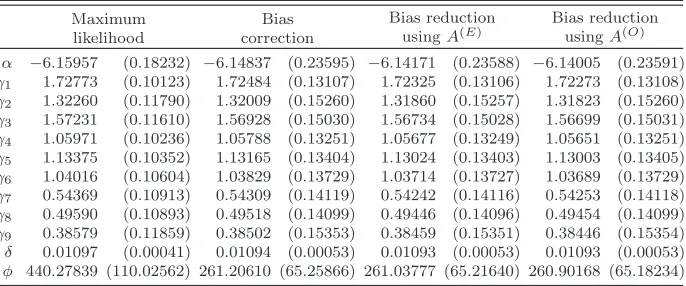
The plots in Figure1give the estimated values of the components ofnjtimes
the bias of ˆβ[j] that correspond to α, γ
100 200 300 400 −0.5 −0.4 −0.3 −0.2 −0.1 0.0
Sample size nj
estimate of n
j
times the bias
α
100 200 300 400
0.00
0.05
0.10
0.15
Sample size nj γ1
100 200 300 400
−0.05
0.00
0.05
0.10
0.15
Sample size nj γ2
100 200 300 400
−0.05
0.00
0.05
0.10
0.15
Sample size nj γ3
100 200 300 400
−0.05
0.00
0.05
0.10
Sample size nj
estimate of n
j
times the bias
γ4
100 200 300 400
−0.05
0.00
0.05
0.10
Sample size nj γ5
100 200 300 400
−0.05
0.00
0.05
0.10
Sample size nj γ6
100 200 300 400
−0.10
−0.05
0.00
0.05
0.10
Sample size nj γ7
100 200 300 400
−0.10
−0.05
0.00
0.05
0.10
Sample size nj
estimate of n
j
times the bias
γ8
100 200 300 400
−0.05
0.00
0.05
0.10
Sample size nj γ9
100 200 300 400
2e−04
4e−04
6e−04
8e−04
Sample size nj δ
[image:12.612.133.473.115.376.2]B(cur) B(Osp)
Fig 1. Simulation-based estimates of the components of nj times the bias of βˆ[j] for
j = 1, . . . ,15. The solid and dashed horizontal lines are the components of B(cur)( ˆβ) and
B(Osp)( ˆβ), respectively. The vertical lines are approximate99%confidence intervals.
1, . . . ,15. To provide an indication of the uncertainty due to simulation error, the estimates are accompanied by 99% confidence intervals based on asymptotic normality. For every parameter the estimate is very close to B(cur)( ˆβ). This experiment provides clear evidence of either an algebraic or implementation error in Ospina et al. [23] as far asb(β) is concerned, at least for the parameters
α, γ1, . . . , γ6andδ; the differences found here are too large to be accounted for by the presentational rounding to 5 decimal places in Table 6 of Ospina et al. [23].
Remark 2: Impact of bias in this example
in detail here, was conducted to check the accuracy of the asymptotic standard errors reported in Table 1: it was found that those standard errors all agree with simulation-based standard errors to at least 3 decimal places. Because of the large bias in the estimated precision parameter ˆφ, the usual standard errors based on the maximum likelihood analysis are systematically too small. The principal effect of bias reduction in this example, then, is to produce more realistic standard errors for the estimates of all the parameters.
It should be noted that the estimated value ofφin this example, even after reduction of the bias, is quite large: that is, the residual dispersion in the model is quite small. This accounts for the rather small bias found in the maximum likelihood estimator for the regression parameters. In a different situation with more substantial residual dispersion present, biases in the regression estimates themselves (i.e., not only in their standard errors) would likely become more important.
Remark 3: Parameterization
In general, bias reduction will typically make most sense when applied to esti-mators whose distribution is approximately symmetric, since it will then most often improve the accuracy of inferences made when using first-order asymp-totic normal approximations. In the present application, the distributions for all parameters exceptφare close to symmetric; ˆφexhibits substantial positive skewness, as is often found in the estimation of positive-valued parameters.
In this model it seems preferable, then, to consider bias reduction instead for a transformed version of φ, the most obvious candidate being logφ. The distribution of log ˆφ is much closer to being symmetric than that of ˆφ, a fact confirmed by graphical summaries (not presented here) of the simulation exper-iment underlying Table2.
Consider a general re-parameterization from β to ω = (α, γ1, . . . , γ9, δ, ζ), with ζ = h(φ) for some appropriate function h : ℜ+ → H ⊂ ℜ. Because the maximum likelihood estimator is equivariant under re-parameterization, the components of the bias vector — and hence of the vector of first-order biases — corresponding toα,γ1, . . . , γ9 and δ will be the same in both the ω and β parameterizations. Assuming thath(.) is at least three times differentiable, and using the consistency of the maximum likelihood estimator ˆφofφ, ˆζ−ζadmits the expansion
ˆ
ζ−ζ=h( ˆφ)−h(φ) = ( ˆφ−φ)dh(φ) dφ +
1 2( ˆφ−φ)
2d2h(φ) dφ2 +
1 6( ˆφ−φ)
3d3h(φ) dφ3 +Op(n
−2).
(4.7) Noting thatE[( ˆφ−φ)r] is O(n−(r+1)/2) if r is odd andO(n−r/2) ifr is even [see, for example24, Section 9.4 for the asymptotic expansion of the maximum likelihood estimator], taking expectations in both sides of (4.7) gives that the bias of ˆζ can be written as
E(ˆζ−ζ) =bφ(β)dh(φ)
dφ +
1 2F
−1
φφ(β)
d2h(φ) dφ2 +O(n
Here bφ(β) and Fφφ−1(β) denote the components of b(β) and {F(β)}−1 which
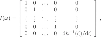
correspond toφ. Furthermore, the expected information matrix onωisF∗(ω) =
J(ω)F(β(ω))J(ω), whereβ(ω) = (α, γ1, . . . , γ9, δ, h−1(ζ)) and
J(ω) =
1 0 . . . 0 0 0 1 . . . 0 0 ..
. ... . .. ... ... 0 0 . . . 1 0 0 0 . . . 0 dh−1(ζ)/dζ
,
withh−1(.) the inverse of the function h(.).
Expression (4.8) can be used to obtain the first-order bias of h( ˆφ) for every
h(.), by merely using the first-order bias of ˆφ, the inverse ofF(β) and the first two derivatives of h(.). Also, the bias-reduced estimate of ω based on A(E) adjustments can be obtained by using iteration (3.4) with
ˆ
ω(j+1)=ω(j)+nF∗ω(j)o−
1
S∗ω(j),
whereS∗(ω) =J(ω)S(β(ω)) is the score vector in theωparameterization. While
the maximum likelihood and bias-corrected estimates forα, γ1, . . . , γ9andδwill be exactly the same in both theβ and ω parameterizations, the corresponding bias-reduced estimates will generally differ slightly between parameterizations. Table 3 gives the maximum likelihood, bias-corrected and bias-reduced es-timates of ω when h(φ) = logφ, along with estimated standard errors based on F∗(ω) evaluated at the corresponding estimates. The principal differences
between Table 3 and Table 1 are in the implied estimates of φ, and con-sequently in the standard errors for estimates of the regression parameters
[image:14.612.218.397.160.226.2] [image:14.612.159.453.514.658.2]α, γ1, . . . , γ9 and δ. For example, the bias-reduced estimate of φ from Table 3
Table 3
Estimates of the parameters of model (4.6) using maximum likelihood, bias correction and bias reduction based onA(E), for the re-parameterization withζ= log(φ). In parentheses are the corresponding estimated standard errors based on the expected information matrixF∗(ω)
Maximum likelihood
Bias correction
Bias reduction usingA(E) α −6.15957 (0.18232) −6.14837 (0.21944) −6.14259 (0.22998)
γ1 1.72773 (0.10123) 1.72484 (0.12189) 1.72347 (0.12777)
γ2 1.32260 (0.11790) 1.32009 (0.14193) 1.31880 (0.14875)
γ3 1.57231 (0.11610) 1.56928 (0.13978) 1.56758 (0.14651)
γ4 1.05971 (0.10236) 1.05788 (0.12323) 1.05691 (0.12917)
γ5 1.13375 (0.10352) 1.13165 (0.12465) 1.13041 (0.13067)
γ6 1.04016 (0.10604) 1.03829 (0.12767) 1.03729 (0.13383)
γ7 0.54369 (0.10913) 0.54309 (0.13133) 0.54248 (0.13763)
γ8 0.49590 (0.10893) 0.49518 (0.13112) 0.49453 (0.13743)
γ9 0.38579 (0.11859) 0.38502 (0.14278) 0.38465 (0.14966)
δ 0.01097 (0.00041) 0.01094 (0.00050) 0.01093 (0.00052)
is exp(5.61608) = 274.8; this is slightly larger than the corresponding value 261.0 from Table 1, resulting in slightly smaller estimated standard errors for the regression parameters in Table3.
5. Concluding remarks
The new algorithm developed here unifies various iterative methods that have been made available previously for specific models, and extends them to cover any new situation for which theO(1/n) bias of the maximum likelihood estima-tor can be derived. The method was tested and demonstrated here in the context of beta-response nonlinear regression, and was found to perform robustly in all of the very large number of samples that were used in simulation studies.
The particular illustrative example presented here is just one of several beta-regression applications that the authors have worked through carefully, and the results were qualitatively the same in all of them. Bias in estimation of the regression parameters in such models is typically so small as to be of no consequence, at least when the precision parameterφis not unreasonably small; but the standard errors in a maximum-likelihood analysis are systematically under-estimated, with the likely consequence that spuriously strong conclusions would often be drawn. Reducing the bias in the estimated precision parameter increases the estimated standard errors in such a way that they reflect better the true variability of the estimated regression parameters.
The calculations described here were all programmed inR[27], and the code is available on request from the first author.
Acknowledgments
The authors gratefully acknowledge the financial support of the UK Engineering and Physical Sciences Research Council for this work.
References
[1] Albert, A. and J. Anderson (1984). On the existence of maximum likelihood estimates in logistic regression models. Biometrika 71(1), 1–10. MR0738319
[2] Breslow, N. E.andX. Lin (1995). Bias correction in generalised linear mixed models with a single component of dispersion.Biometrika 82, 81–91. MR1332840
[3] Bull, S. B., C. Mak,andC. Greenwood(2002). A modified score func-tion estimator for multinomial logistic regression in small samples. Com-putational Statistics and Data Analysis 39, 57–74.MR1895558
[5] Cordeiro, G. and M. Toyama Udo (2008). Bias correction in gen-eralized nonlinear models with dispersion covariates. Communications in Statistics: Theory and Methods 37(14), 2219–225.MR2526676
[6] Cordeiro, G. M. and P. McCullagh (1991). Bias correction in gen-eralized linear models. Journal of the Royal Statistical Society, Series B: Methodological 53(3), 629–643.MR1125720
[7] Cordeiro, G. M.andK. L. P. Vasconcellos(1997). Bias correction for a class of multivariate nonlinear regression models. Statistics & Probability Letters 35, 155–164.MR1483269
[8] Cox, D. R. and D. V. Hinkley(1974). Theoretical Statistics. London: Chapman & Hall Ltd. MR0370837
[9] Cox, D. R.andE. J. Snell(1968). A general definition of residuals (with discussion). Journal of the Royal Statistical Society, Series B: Methodolog-ical 30, 248–275.MR0237052
[10] Cribari-Neto, F.andA. Zeileis(2010). Beta regression in R. Journal of Statistical Software 34(2), 1–24.
[11] Efron, B. (1975). Defining the curvature of a statistical problem (with applications to second order efficiency) (with discussion). The Annals of Statistics 3, 1189–1217.MR0428531
[12] Ferrari, S. and F. Cribari-Neto (2004). Beta regression for mod-elling rates and proportions. Journal of Applied Statistics 31(7), 799–815. MR2095753
[13] Firth, D. (1992). Bias reduction, the Jeffreys prior and GLIM. In L. Fahrmeir, B. Francis, R. Gilchrist, and G. Tutz (Eds.), Advances in GLIM and Statistical Modelling: Proceedings of the GLIM 92 Conference, Munich, New York, pp. 91–100. Springer.
[14] Firth, D. (1993). Bias reduction of maximum likelihood estimates. Biometrika 80(1), 27–38.MR1225212
[15] Gart, J. J., H. M. Pettigrew,and D. G. Thomas(1985). The effect of bias, variance estimation, skewness and kurtosis of the empirical logit on weighted least squares analyses. Biometrika 72, 179–190.
[16] Heinze, G. and M. Schemper (2002). A solution to the problem of separation in logistic regression. Statistics in Medicine 21, 2409–2419. [17] Heinze, G.andM. Schemper(2004). A solution to the problem of
mono-tone likelihood in Cox regression. Biometrics 57, 114–119.MR1833296 [18] Kosmidis, I. (2009). On iterative adjustment of responses for the
reduc-tion of bias in binary regression models. Technical Report 09-36, CRiSM working paper series.
[19] Kosmidis, I.and D. Firth (2009). Bias reduction in exponential family nonlinear models. Biometrika 96(4), 793–804.MR2564491
[20] Lin, X. and N. E. Breslow (1996). Bias correction in generalized lin-ear mixed models with multiple components of dispersion. Journal of the American Statistical Association 91, 1007–1016.MR1424603
[22] Mehrabi, Y.andJ. N. S. Matthews(1995). Likelihood-based methods for bias reduction in limiting dilution assays. Biometrics 51, 1543–1549. [23] Ospina, R., F. Cribari-Neto, and K. L. Vasconcellos (2006).
Im-proved point and interval estimation for a beta regression model. Compu-tational Statistics and Data Analysis 51(2), 960 – 981.MR2297500 [24] Pace, L.andA. Salvan(1997). Principles of Statistical Inference: From
a Neo-Fisherian Perspective. London: World Scientific.MR1476674 [25] Pettitt, A. N., J. M. Kelly, and J. T. Gao(1998). Bias correction
for censored data with exponential lifetimes. Statistica Sinica 8, 941–964. MR1651517
[26] Prater, N. H. (1956). Estimate gasoline yields from crudes. Petroleum Refiner 35, 236–238.
[27] R Development Core Team(2008). R: A Language and Environment for Statistical Computing. Vienna, Austria: R Foundation for Statistical Computing. ISBN 3-900051-07-0.
[28] Sartori, N.(2006). Bias prevention of maximum likelihood estimates for scalar skew normal and skewtdistributions.Journal of Statistical Planning and Inference 136, 4259–4275.MR2323415
[29] Schaefer, R. L. (1983). Bias correction in maximum likelihood logistic regression. Statistics in Medicine 2, 71–78.
[30] Simas, A. B., W. Barreto-Souza,andA. V. Rocha(2010). Improved estimators for a general class of beta regression models. Computational Statistics and Data Analysis 54(2), 348–366.
[31] Smithson, M. and J. Verkuilen (2006). A better lemon squeezer? Maximum-likelihood regression with beta-distributed dependent variables. Psychological Methods 11(1), 54–71.
![Fig 1. Simulation-based estimates of the components ofB nj times the bias ofβˆ[j] forj = 1,](https://thumb-us.123doks.com/thumbv2/123dok_us/9694322.470742/12.612.133.473.115.376/fig-simulation-based-estimates-components-times-bias-ofb.webp)