University of Warwick institutional repository: http://go.warwick.ac.uk/wrap
This paper is made available online in accordance with publisher policies. Please scroll down to view the document itself. Please refer to the repository record for this item and our policy information available from the repository home page for further information.
To see the final version of this paper please visit the publisher’s website. Access to the published version may require a subscription.
Author(s): Pavlo Blavatskyy and Ganna Pogrebna
Article Title: Endowment effects? “Even” with half a million on the table! Year of publication: 2009
Link to published article:
http://dx.doi.org/10.1007/s11238-009-9152-4
Endowment Effects?
“Even” with Half a Million on the Table!
∗Pavlo Blavatskyy
†and Ganna Pogrebna
‡April 2009
Abstract
In the television show Deal or No Deal a contestant is endowed with a sealed box
containing a monetary prize between one cent and half a million euros. In the course of
the show the contestant is offered to exchange her box for another sealed box with the
same distribution of possible monetary prizes inside. This offers a unique natural
experiment for studying endowment effects under high monetary incentives. We find
only weak endowment effects when contestants exchange their box for another box with
the same distribution of possible prizes.
Key words: endowment effect, expected utility theory, prospect theory, television show
JEL Classification codes: C93, D81
∗
We are grateful to Colin Camerer and Richard Thaler for their advice and helpful suggestions. We thank Steffen Andersen, Daniela Di Cagno, Christian Ewerhart, Anita Gantner, Lorenz Goette, Glenn Harrison, John Hey, Rudolf Kerschbamer, Wolfgang Koehler, Morten Lau, Charles Plott, Ulrich Schmidt, Francesco Trebbi, Nathaniel Wilcox and Peter Wakker for their comments. We also thank participants of research seminars at Humboldt University in Berlin (May 2007), the University of Zurich (December 2006), Max Planck Institute for Research on Collective Goods in Bonn (October 2006), the University of Bonn (September 2006), and the University of Innsbruck (May 2006), participants of the Augustin Cournot Doctoral Days in Strasbourg, France (April 2007),the Economic Science Association European Meeting in Nottingham, United Kingdom (September 2006) and the 12th International Conference on The Foundation and Application of Utility, Risk and Decision Theory in Rome, Italy (June 2006). We are grateful to Anabela Botelho and Glenn Harrison, who generously provided data from the French version of Deal or No
Deal. We have benefited from extensive discussions with, and helpful suggestions from, Thierry Post and Guido Baltussen. Pavlo Blavatskyy acknowledges financial support from the Fund for Support of
Academic Development at the University of Zurich. Previos version of this paper was sirculated under the title “Loss Aversion? Not with Half a Million on the Table!”
†
Corresponding author, Institute for Empirical Research in Economics, University of Zurich,
Winterthurerstrasse 30, CH-8006 Zurich, Switzerland, tel.: +41(0)446343586, fax: +41(0)446344978, e-mail: [email protected]
‡
Endowment Effects?
“Even” with Half a Million on the Table!
1. Introduction
Substantial experimental evidence from economics and psychology suggests that
initial endowments have an impact on human preferences. Endowment effect (Thaler
(1980)) says that when people come to own a good, they tend to value it more than they
did before they owned it (Kahneman et al. (1991)). For example, Kahneman et al. (1990)
find that students, who were given mugs worth $6 each, were willing to sell them at a
median price of $7 each. At the same time, students, who did not come to possess the
mugs, were willing to buy them at a median price of $3.50 per mug. While many
experiments replicate this result, several studies treat the endowment effect as an
inexperienced consumer’s mistake, which disappears in the process of learning (e.g. Knez
et al.(1985),Coursey et al.(1987),Brookshire and Coursey (1987),Shogren et al.(1994).
In a field experiment, List (2004) finds that professional dealers on the sports card
market are more likely to accept the swap offer than inexperienced consumers. List
(2004) argues that consumers facing decision problem, which they have experienced
before, may overcome the endowment effect. In a similar vein, Myagkov and Plott (1997)
find that risk-seeking behavior over losses, predicted by prospect theory, tends to
decrease with experience in a market setting. Plott and Zeiler (2007) show that
asymmetries in exchange behavior disappear if an experimenter controls for subject
misconceptions by introducing incentive-compatible elicitation device, subject training in
the task, paid practice rounds and subject anonymity. This paper contributes to this
literature by showing that individuals exhibit only weak endowment effects if they make
decisions involving high stakes, even without prior practice or training and when their
We use the natural experiment of the television show Deal or No Deal to analyze
endowment effects when stakes are large. Deal or No Deal is produced by the media
company Endemol in 44 countries worldwide. In this paper we analyze French, Italian
and British versions of the show. Deal or No Deal contestants are endowed with a sealed
box, containing an unknown monetary prize. The maximum prize is €500,000 in France
and Italy and £250,000 in the UK.
During the show, contestants have a possibility to exchange their box for another
box with the same distribution of possible prizes inside.1 This provides a unique natural
experiment to test endowment effects in a previously unexplored domain – when lotteries
involve large outcomes. The importance of large stakes is apparent in Blavatskyy and
Pogrebna (2008) who find that, in contrast to numerous laboratory studies with low
monetary incentives, British and Italian Deal or No Deal contestants do not exhibit lower
risk aversion when facing gains of low probability.
We find that in all three versions of the show, Deal or No Deal contestants exhibit
only weak endowment effects. The swap offer is accepted by 73%, 47% and 43% of
contestants who receive exchange offers in the French, Italian and British version of the
show respectively. This finding suggests that people may overcome endowment effects
under high monetary incentives.
The remainder of this paper is organized as follows. Section 2 describes television
show Deal or No Deal. Data are presented in Section 3. Section 4 derives the theoretical
predictions of expected utility, regret and prospect theory. Section 5 presents our main
empirical findings. Section 6 concludes.
1
2. Description of the Television Show
French, Italian and British versions of the Deal or No Deal television show have
the following common features. Several contestants, each representing one of the
administrative regions of the country, participate in every television episode. All
contestants self-select into the show by submitting an application for participation either
through the national Deal or No Deal web site or by calling the selection center in their
country.
Contestants are randomly assigned identical sealed boxes, numbered
consecutively from the first to the last. Boxes contain monetary prizes, ranging from very
small to very large. Monetary prizes are allocated across boxes by the independent notary
company. Contestants know the list of possible prizes at any point in the show but they
do not know the content of each box.
The show consists of two stages. During the first (preliminary) stage, one
contestant is selected to play the game. Remaining contestants (waiting contestants)
continue to participate in the next television episode. The contestant, selected to play the
game, is replaced by a new representative of the same region. New contestant is selected
from a pool of volunteers who applied for the participation.
The second stage is the game itself. During the game, a contestant keeps her own
box and opens the remaining boxes one by one. When a box is opened, the prize hidden
inside is publicly revealed and eliminated from the list of possible prizes.
After opening several boxes a contestant receives an offer from the “bank”. The
offer could be either a monetary price for the content of her box or the possibility to
exchange her box for any of the remaining sealed boxes. If a contestant is offered to swap
not selected by the producers, the audience or other contestants). In this paper we analyze
contestants’ decisions whether to accept or reject the exchange offer.
The game terminates when either the contestant accepts the price offered by the
“bank” or when all boxes are opened. In the latter case, the contestant leaves with the
content of her box, which is opened last. The game does not terminate when the
contestant accepts (or rejects) the exchange offer. Irrespective of the contestant’s decision
on the exchange offer, she must continue opening remaining sealed boxes one by one
until the “bank” makes another offer or all boxes are opened.
2.1. French Version
À Prendre ou à Laisser is the French version of Deal or No Deal. It is aired every
weeknight on the channel TF1 of the French television. The show features 22 contestants
from 22 different regions of France, holding identical boxes. Each box contains a
randomly assigned monetary prize, ranging from €0.01 to €500,000.2 The list of possible
prizes is given on Figure 1. For entertainment purposes, three low monetary prizes are
substituted by token gifts (e.g. a cup for €5 or a puppy for €100). Boxes are assigned to
the contestants by an independent adjudicator, who is present in the studio during the
show.
[INSERT FIGURE 1 HERE]
During the preliminary stage, contestants receive one general knowledge selection
question with three possible answers (A, B and C). One of contestants, who answered this
question correctly, is selected to play the game. However, the criteria for the selection
procedure (e.g. “fastest finger”, random selection, longest waiting time on the show) are
not revealed to the public.
2
In the French version of Deal or No Deal one of the prizes is a “Joker” - an
episode-specific variable. The “Joker” is determined in the beginning of the show by
multiplying the number of correct answers to the selection question, given by contestants
in the preliminary stage, by €10,000. The amount of the “Joker” is instantaneously added
to the list of possible prizes.3
In the French version of the show contestants receive offers from the “bank” after
opening 6, 3, 3, 3, 3 and 2 boxes respectively. Another peculiarity of this version is that
the exchange offers are fairly frequent (up to four exchange offers per episode). However,
there is no requirement for the “bank” to make any exchange offers to the contestant
during a television episode.
2.2. Italian Version
Affari Tuoi is a daily television show, broadcasted on the first channel of Italian
television RAI Uno. Twenty contestants participate in every episode. Every contestant is
randomly assigned one box that contains one of twenty monetary prizes ranging from
€0.01 to €500,000 (Figure 2). Four low prizes are substituted with the token gifts. Similar
to the French version, independent notary company assigns boxes to contestants. Before
February 11, 2006, contestants received offers from the “bank” after opening 6, 3, 3, 3
and 3 boxes correspondingly. Starting from February 11, 2006, the “bank” makes offers
after a contestant opens 3, 3, 3, 3, 3, 1, 1, and 1 box respectively.
[INSERT FIGURE 2 HERE]
In every episode, the contestant receives at least one offer to exchange her box.
Official rules of the show require the “bank” to offer exchange option at least once in
3
every television episode. Therefore, the first offer that the “bank” makes to the contestant
is always the exchange offer.4 Since the “bank” always proposes exchange in the first
offer, irrespective of the distribution of the remaining prizes or the personality of the
contestant, the first exchange offer is always uninformative i.e. it does not provide any
information about possible content of the contestant’s box.5
Occasionally (in 28% of all episodes in our sample), the contestant also receives
the second offer to exchange her box. The “bank” typically offers the second exchange
opportunitywhen thereareonlytwo sealed boxes left (including the box in the possession
of the contestant).6 The second exchange offer is made at the discretion of the “bank”
(official rules of the show do not regulate when the “bank” should offer second exchange
possibility). However, in our recorded sample the “bank” offers the second exchange
option almost equally frequently when the prize inside the contestant’s box is above and
below the median of the distribution of possible prizes. Thus, the second exchange offer
is uninformative i.e. contestants cannot infer new information about the prize hidden
inside their box upon observing the second exchange offer.
2.3. British Version
Deal or No Deal UK is aired on Channel 4 of the British television. Twenty two
contestants from different parts of the UK participate in every episode.7 The prizes range
4
Before February 11, 2006, the first offer was always made after the contestant opened six boxes. Starting from February 11, 2006, the first offer was made after the contestant opened three boxes.
5
According to Bombardini and Trebbi (2005), the “bank” in the Italian version of Deal or No Deal is informed about the prize sealed inside the contestant’s box and can potentially make informative offers.
6
Such offers constitute 71% of all cases when the “bank” proposes the second exchange opportunity. In 18% (7%) of the cases the second exchange offer is made when five (eight) unopened boxes are left. In one episode exchange is offered when four unopened boxes are left.
7
from £0.01 to £250,000 (Figure 3).8 They are randomly assigned to 22 boxes by an
independent adjudicator. However, an independent adjudicator does not assign boxes to
contestants. After the prizes are distributed across boxes and boxes are sealed, contestants
choose their boxes at random by drawing numbered ping-pong balls.
[INSERT FIGURE 3 HERE]
The British version of the show does not have a selection phase. The contestant is
pre-selected by the producers and, therefore, it is quite rare for contestants to wait for
more than 30 shows before they receive an opportunity to play the game. However,
waiting contestants do not know in advance when they will be selected.
The game itself follows a similar procedure as in France and Italy: contestants
receive offers after opening 5, 3, 3, 3, 3, and 3 boxes respectively. However, there are
three major differences. First, the contestants in Deal or No Deal UK rarely receive
exchange offers. As a rule, the “bank” offers to exchange the box when there are only
two unopened boxed left and the contestant rejects the last monetary offer.9
Second, in Deal or No Deal UK the contestant may take advice from waiting
contestants or suggestions from the host on the next box to be opened or on whether to
accept or reject the deal from the “bank”. This is very different from the procedure in
France and Italy, where it is observed by the representative of the independent notary
company, present on the show, that contestant’s decision to open a certain box or to
accept or reject the monetary offer of the “bank” is not precipitated by the suggestions of
waiting contestants or the host. Moreover, while in Deal or No Deal UK the contestant is
allowed to change her mind about opening a certain box after she has already called out
its number, in France and Italy contestants do not have this opportunity.
8
At the time of the broadcasts the exchange rate was £1= €1.48.
9
3. Data
The data set, analyzed in this paper, consists of 49 television episodes of the
French version, 100 episodes of the Italian version and 355 episodes of the British
version of Deal or No Deal. Only one contestant plays the game in every episode. French
episodes have been broadcasted from January 3rd, 2006 till April 10th, 2006 on channel
TF1.10 Italian episodes have been aired from September 20th, 2005 to February 13th, 2006
on channel RAI Uno.11 British episodes have been broadcasted from October 31st, 2005
to January 12th, 2007 on Channel 4 of the British television.12 Table 1 summarizes
selected descriptive statistics for French, Italian and British contestants in our data set.
Descriptive Statistics French version Italian version British version
Percent of female 71% 55% 50%
Average age (years) 28 47 41
Percent of married 39% 81% 51%
Average earnings €71,579 €30,363 £16,763
Median earnings €50,000 €20,000 £12,900
Average number of exchange
[image:10.612.84.529.318.450.2]offers per contestant 1.86 1.29 0.18
Table 1 Selected descriptive statistics for French, Italian and British contestants
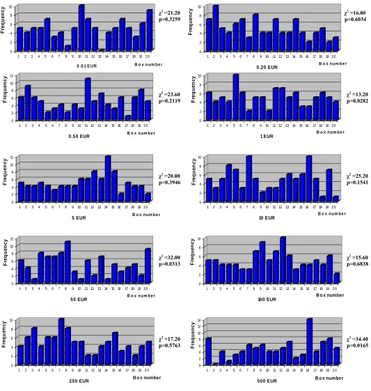
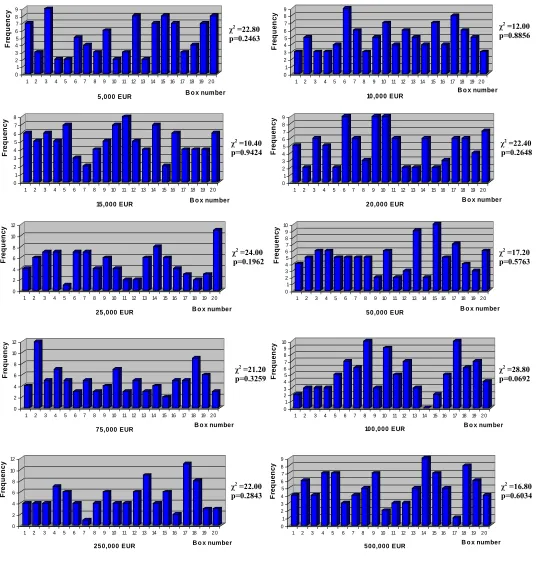
Dealor No Deal regulations state that prizes are allocated across boxes at random.
We checked if prizes are equally likely to appear inside each box. In our data set the
distributionofprizesacrossboxesisnotsignificantlydifferentfromauniformdistribution
at 1% significance level (e.g. Figures 4 and 5 for Affari Tuoi). Thus, there is no apparent
reason for misconceptions that large prizes are more likely to be inside particular boxes.
[INSERT FIGURES 4 AND 5 HERE]
10
French episodes were recorded by Professor Anabela Botelho who generously shared the data with us.
11
Italian episodes were recorded by the authors.
12
A significant portion of British data was compiled from http://donduk.blogspot.com/2006/06/previous-game-reports.html and related Internet sources. We have also watched several episodes, available online, including the Hall of Fame editions of the show with Deal or No Deal UK highlights.We are particularly grateful to Dave Woollin for collecting show statistics and publishing it on http://www.screwthebanker.com
4. Theoretical Prediction
Expected utility theory and many generalized non-expected utility theories such
as, for example, regret theory predict that an individual is exactly indifferent between
keeping her own box and exchanging it for any of the remaining identical sealed boxes.
However, (cumulative) prospect theory predicts that an individual should always reject
the exchange offer due to the assumption of loss aversion. First, we will derive these
theoretical predictions for a static decision problem when contestants evaluate a risky
lottery as a lottery that delivers each of the possible prizes (that have not yet been
eliminated from the game) with equal probability. Then we will consider a dynamic case,
when contestants evaluate a risky lottery taking into account the expectation of future
“bank” offers that they will receive in the course of the game.
4.1. Static Decision Problem
4.1.1. Expected Utility Theory
According to expected utility theory, an individual should be exactly indifferent
between keeping her box and exchanging it for any of the remaining sealed boxes.
Consider a contestant who is offered an exchange when there are N sealed boxes each
containing one of the prizes x1 <x2 <...< xN . If an individual keeps her box, she obtains
expected utility
∑
iN=u(
w+xi)
N 1
1
, where u
()
. is a von Neumann-Morgenstern utilityfunction of the contestant and w is her private wealth.
If the contestant exchanges her box that contains prize xi, i∈
{
1,...,N}
, for one ofthe remaining sealed boxes, she obtains expected utility
(
j)
i j
N
j u w x
N−
∑
≠=1 +1 1
. The
to be inside her box. Therefore, after exchanging the boxes, the contestant receives
expected utility
(
)
(
−)
(
(
+)
−(
+)
)
= = + −∑ ∑
∑
=∑
= = ≠= N i i N j j N i j i j Nj u w x N N u w x u w x
N
N 1 1 1 1 1
1 1 1 1
(
)
∑
= += iN u w xi
N 1
1
. Thus, the contestant receives exactly the same expected utility after
exchanging her box as after keeping her initial box. In other words, according to expected
utility theory there is no reason why the contestant should accept or reject an offer to
exchange her box for one of the remaining sealed boxes.
4.1.2. Regret Theory
Many generalized non-expected utility theories also predict that an individual is
indifferent between accepting and rejecting swap offer. For example, according to regret
theory an individual always accepts exchange offer if
(
1)
(
,)
01
1 1 >
−
∑ ∑
=≠=
N
i i j
i j N
j x x
N
N ψ ,
where ψ
( )
⋅,⋅ is a skew-symmetric utility function i.e. ψ(
xi,xj)
=−ψ(
xj,xi)
(e.g. Loomesand Sugden, 1987). It is easy to see that
∑ ∑
=(
)
=∑ ∑
= −=(
)
+≠=
N
i i j
i j N
i i j
i j N
j x x 2 x x
1 1
1 1ψ , ψ ,
(
,)
(
,)
(
,)
01 1 1 2 1 1 1
1 1 = − =
+
∑ ∑
=− =+∑ ∑
= −=∑ ∑
N=+ =−i
j j i
N i N
i i j
i j N
i i j
N i
j ψ x x ψ x x ψ x x . Thus, according
to regret theory a contestant is exactly indifferent between accepting and rejecting the
exchange offer. The intuition behind this result is simple. A contestant who accepts the
exchange offer experiences ex post regret when she discovers at the end of the show that
her initial box contained a larger prize. However, a contestant who rejects the exchange
offer experiences exactly the same ex post regret when she opens all boxes only to
discover that her initial box contains a smaller prize than one of the boxes that she could
4.1.3. (Cumulative) Prospect Theory
In prospect theory, an individual derives utility from changes in her asset position
relative to a reference point (e.g. Kahneman and Tversky (1979)). Prospect theory does
not specify what constitutes a reference point in a particular decision problem. In this
section we show that an individual should never exchange her own box for any of the
remaining sealed boxes irrespective of the location of a reference point. This theoretical
prediction is driven by the assumption of loss aversion.
A contestant who rejects the exchange offer and keeps her box derives zero utility
since her asset position does not change (relative to any reference point). Now consider a
contestant who accepts the exchange offer. Let w be her private wealth (excluding the
content of her box) and let xi,i∈
{
1,...,N}
, denote a prize inside her box before exchange.Let v
()
. be the value function that measures utility from changes in wealth relative to areference point. The value function is normalized so that v
( )
0 =0. Prospect theoryassumes that individuals are loss averse so that the value function is steeper for losses
than for gains i.e. v
( )
x <−v( )
−x for any x>0 (e.g. Kahneman and Tversky (1979)).Although prospect theory does not specify the location of a reference point, it
assumes that individuals incorporate their initial endowments into their reference point
(e.g. Kahneman et al. (1991), Tversky and Kahneman (1991)).13 Thus, in the context of
this natural experiment, we can write a reference point as r+xi, where r is constant.
Notice that r=w is a special case corresponding to the original version of prospect
13
Notice that if a contestant swaps boxes due to her subjective belief that her initial box contains a low prize, she may be expected to open an old box immediately after exchange. Interestingly, 90% of
theory in Kahneman and Tversky (1979) where a reference point is assumed to be equal
to a current asset position. A recently proposed model of Koszegi and Rabin (2006)
corresponds to a special case when constant r equals to the private wealth of a contestant
w plus her (unobservable) rational expectation of future earnings in Deal or No Deal. In
the remainder of the paper we will assume that r≥w.
According to the cumulative prospect theory, a contestant who exchanges her own
box with prize xi for a box with a lower prize xj, j∈
{
1,...,i−1}
obtains utility(
)
[
(
(
j i)
)
(
(
j i)
)
]
i
j v w+ xj −r −xi ⋅w− ≤w+ x −r−x −w− <w+ x −r −x
− =
∑
11 Pr δ Prδ , where[ ] [ ]
0,1 0,1: →
−
w is the probability weighting function for losses (Tversky and Kahneman
(1992)) and Pr
(
δ <w+xj −r−xi)
denotes the probability that the change in wealth δduring theswapof boxes(relative toa reference point r+xi)islowerthan w+xj −r−xi.
Finally, according to the cumulative prospect theory, a contestant who exchanges
her own box with prize xi for a box with a higher prize xj, j∈
{
i+1,...,N}
obtains utility(
)
[
(
(
j i)
)
(
(
j i)
)
]
N i
j=+ v w+xj −r−xi ⋅w+ ≥ w+x −r−x −w+ >w+x −r−x
∑
Pr δ Pr δ1 , where
[ ] [ ]
0,1 0,1: →
+
w is the probability weighting function for gains. The contestant does not
know the prize xi sealed inside her box but she knows that each prize x1,...,xN is likely
to be inside her box. Effectively, she has a stochastic reference point, and her ex ante
utility from exchanging the boxes is given by
(
)
[
(
(
)
)
(
(
)
)
]
∑ ∑
= − −−
= + − − ⋅ ≤ + − − − < + − − +
= iN ij v w xj r xi w w xj r xi w w xj r xi
U 1 1
1 Prδ Prδ
(
)
[
(
(
)
)
(
(
)
)
]
∑ ∑
= =+ + − − ⋅ + ≥ + − − − + > + − −+ iN1 Nj i 1v w xj r xi w Prδ w xj r xi w Prδ w xj r xi or,
(1)
{
(
)
[
(
(
)
)
(
(
)
)
]
(
)
[
(
Pr(
)
)
(
Pr(
)
)
]
}
Pr Pr 1 1 1 w r x x w w r x x w w r x x v r w x x w r w x x w r w x x v U j i j i j i N i i
j j i j i j i
− + − > − − + − ≥ ⋅ − + − + + − + − < − − + − ≤ ⋅ − + − = + + = − = − −
∑ ∑
δ δ δ δSince all prizes are randomly distributed across the boxes, when two boxes are
exchanged, every positive change in wealth is equally likely as a negative change in
wealth of the same absolute amount (relative to the same reference point).In other words,
(
δ ≥xi−xj+r−w) (
=Prδ ≤xj−xi+w−r)
Pr and Pr
(
δ>xi−xj+r−w) (
=Prδ<xj−xi+w−r)
for every xi >xj and r≥w. The assumption of loss aversion additionally implies that
(
x x r w)
v(
x x w r)
v i − j+ − <− j − i+ − for every xi >xj and r≥w. Using these two
results we can rewrite equation (1) as an inequality
(2)
(
)
[
(
(
)
)
(
(
)
)
(
)
(
x x w r)
w(
(
x x w r)
)
]
w r w x x w r w x x w r w x x v U i j i j i j i j N i i
j j i
− + − < + − + − ≤ − − − + − < − − + − ≤ ⋅ − + − < + + − − = − =
∑ ∑
δ δ δ δ Pr Pr Pr Pr 1 1 1Previous experimental studies demonstrate that the probability weighting function
typically has a similar shape for gains and losses but it is more curved for gains and more
linear for losses (e.g. Tversky and Kahneman (1992), Abdellaoui (2000)). We will
assume that there exist probability q≤1 2 such that
(
p)
w( )
p w(
p)
w( )
pw+ +ε − + ≥ − +ε − − for any p,p+ε∈
[ ]
0,q and(
p)
w( )
p w(
p)
w( )
pw+ +ε − + ≤ − +ε − − for any p,p+ε∈
[ ]
q,1 . Inequality (2) thenimmediately implies that U < 0 i.e. the contestant derives a strictly negative utility from
exchanging her box for one of the remaining sealed boxes. In other words, according to
prospect theory an individual has a strong reason not to exchange her box: the value of
exchange is strictly negative because a loss averse individual expects more aggravation
4.2. Dynamic Decision Problem
In a dynamic decision problem, contestants take into account future “bank” offers
that they are likely to receive in course of the game. A contestant facing prizes x1 and x2
hidden in two unopened boxes perceives them as a risky lottery L
(
x1,12;x2,12)
just asin a static decision problem.14 The contestant facing prizes x=
{
x1,...,xN}
hidden in2 >
N unopened boxes perceives them as a risky lottery L
( )
x . Let m denote the numberof boxes that the contestant has to open before the next “bank” offer is made (m is either
2 or 3 in the French version, m is either 1 or 3 in the Italian version and m=3 in the
British version of Deal or No Deal). There are CNN−m =N!
(
m!(
N−m)
!)
combinations ofprizes x that the contestant can face when the next offer is made. Let us denote these
combinations by N
m N C 1 x x −
,..., . Lottery L
( )
x is then recursively defined by(3)
( )
∑
[
( )
(
(
( )
)
( )
( )
)
( )
(
(
( )
)
( )
( )
)
]
∑
( )
− −
= − =
−
−
− ≥ + < +
− =
N m
N NNm
C i C i i N m N m N i i i i i i N m N m N L C O u L u I O O u L u I L C L 1 1 , ˆ ˆ ˆ ˆ ˆ 1 x x x x x x x
x π π
where Oˆ
( )
xi is the expectation of a future monetary offer for xi prizes left in theunopened boxes, πˆN−m is the expected probability that the “bank” offers an exchange
option instead of a monetary amount at the stage when N−m boxes remain unopened
and I
( )
x is an indicator function i.e. I( )
x =1 if x is true and I( )
x =0 if x is false.15 Forthe sake of our argument, an anticipated future offer Oˆ
( )
xi can be either a probabilitydistribution over possible monetary amounts or a monetary amount for certain.
14
In French, Italian and British versions of Deal or No Deal the “bank” does not make any further monetary offers when a monetary offer for two prizes is rejected. Thus, in this case dynamic and static decision problems coincide because there are no anticipated “bank” offers in the future.
15
For any two lotteries L1
(
y1,p1;...;yk,pk)
and L2(
z1,q1;...;zl,ql)
a compound lottery(
)
21 1 L
L α
α + − , α∈
[ ]
0,1, is defined in the usual way—it yields outcome yi with probability α⋅pi,{
k}
4.2.1. Expected Utility Theory
Consider a contestant who is offered an exchange when there are N sealed boxes
with remaining prizes x=
{
x1,...,xN}
. If N =2, this contestant obtains expected utility( )
(
L) (
u w x1)
2 u(
w x2)
2u x = + + + from rejecting the exchange offer. If N >2, utility
from rejecting the swap offer can be calculated through a Bellman optimality equation
(4)
(
( )
)
∑
[
(
)
{
(
( )
)
( )
( )
}
(
( )
)
]
− = − − − + − = N m N C i i m N i i m N N m N L u O u L u C L u 1 ˆ ˆ , max ˆ 1 1 x x x
x π π .
Now consider the case when the contestant exchanges her old box for the new box
with prize xj, j∈
{
1,...,N}
sealed inside. If N =2, this contestant obtains expected utility( )
(
L) (
u w x1)
2 u(
w x2)
2u x = + + + after accepting the exchange offer. If N >2, there
are CNN−−11−m =
(
N−1)
!(
m!(
N−1−m)
!)
=CNN−m N combinations of prizes x, all of whichinclude prize xj, that the contestant can face when the next offer is made. Let us denote
these combinations by
j
j x
x C N
1 N m N x x −
,..., . Utility from accepting the exchange offer
(conditional on the prize xj being inside the new box) is then given by Bellman equation
(5)
( )
( )
∑
[
(
)
{
(
( )
) ( )
(
)
}
(
( )
)
]
−
= − −
−
+ −
= C N
i x i m N x i x i m N N m N x N m N j j j
j C uL uO u L
N L u 1 ˆ ˆ , max ˆ
1 x x x
x π π
Since the contestant does not know which prize is sealed inside her new box and
prizes are distributed across boxes at random, expected utility after accepting exchange is
given by
∑
N=( )
( )
j uL xj
N 1
1
x , where conditional expected utility
( )
( )
j
x
L
u x is defined in (5).
Notice that
{
N}
m N N
m
N N 1 C
C
1 x x x
x − − ⎭⎬= ⎫ ⎩ ⎨ ⎧
=1 ,..., ,...,
U
Nj x xj
j and expected utility after accepting
exchange offer can be re-written as (4). Thus, in a dynamic decision problem expected
4.2.2. (Cumulative) Prospect Theory
In a dynamic decision problem, similarly to a static decision problem, contestants
obtain zero utility from rejecting the exchange offer because their asset position does not
change relative to any reference point that they may adopt. Next we show that contestants
receive a strictly negative utility from accepting the exchange offer. If there are only two
unopened boxes left with prizes x1 and x2 sealed inside, a contestant, who accepts the
exchange offer, derives utility v
(
w+x1 −r−x2) ( ) (
w− 12 +v w+x2 −r−x1) ( )
w+ 1 2 <(
+ 2− − 1) ( ) (
12 + + 2− − 1) ( ) (
12 ≤ + 2− − 1) ( )
[
12 −( )
12]
≤0−
< vr x w x w− vw x r x w+ vr x w x w+ w− ,
with the first (strict) inequality due to the assumption of loss aversion.
If there are N >2 unopened boxes left, a contestant faces a lottery recursively
defined by (3). Notice that we cannot write Bellman equation (4) because (cumulative)
prospect theory does not satisfy the independence axiom of expected utility theory. Let
(
z p zM qM)
L 1, 1;...; , denote the reduced form of a compound lottery, which is recursively
defined in(3).According to(cumulative)prospect theory,utilityof this lotteryis given by
(
)
[
(
(
)
)
(
(
)
)
]
∑ ∑
= = + − − ⋅ − ≤ + − − − − < + − − +=
<
N
i j i j i
M
i
j w w z r x w w z r x
j vw z r x
U
i x j z
1 1 Prδ Prδ
(
)
[
(
(
)
)
(
(
)
)
]
∑ ∑
= = + − − ⋅ + ≥ + − − − + > + − −+
>
N
i j i j i
M
i
j w w z r x w w z r x
j v w z r x
i x j z
1 1 Prδ Prδ .
If prizes are distributed across boxes at random and contestants’ expectation of
future monetary offers depends only on the set of possible prizes,16 every positive change
in wealth during the swap is equally likely as a negative change in wealth of the same
absolute amount (relative to the same reference point).Following the derivation presented
in section 4.1.3 we can easily show that U <0 due to the assumption of loss aversion.
16
5. Results
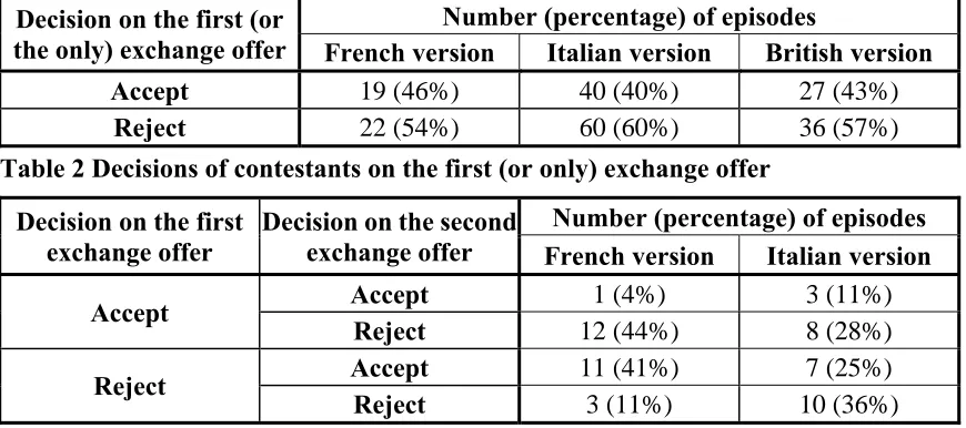
Tables2and3showthedecisionsofcontestantsonthefirst(or theonly)exchange
offer and the second exchange offer respectively. The second swap opportunity is offered
only in French and Italian versions of Deal or No Deal. It is accepted in 45% of cases in
the French version and in 36% of cases—in the Italian version. Observed decisions are
quite similar across all three versions even through French contestants typically receive
several swap offers, Italian contestants are guaranteed to get at least one exchange
opportunity and only one fifth of British contestants are given the chance to swap boxes.
High percentage of contestants, who accept the exchange offer and do not keep
their initial endowment, shows that contestants exhibit rather weak endowment effects.
Contestants who accept at least one exchange offer do not reveal endowment effects.
Contestants who rejected all swap offers do not necessarily exhibit an endowment effect.
Thus,contestants,who accept the first (or the only) exchange offer, and contestants, who
reject the first offer but accept the second offer, are not averse to losses. 73% of French
contestants, 47% of Italian contestants and 43% of British contestants, who receive the
exchange offer in our data set, clearly reveal no endowment effect.17
Decision on the first (or the only) exchange offer
Number (percentage) of episodes
French version Italian version British version
Accept 19 (46%) 40 (40%) 27 (43%)
[image:19.612.90.525.463.656.2]Reject 22 (54%) 60 (60%) 36 (57%)
Table 2 Decisions of contestants on the first (or only) exchange offer
Decision on the first exchange offer
Decisiononthesecond exchange offer
Number (percentage) of episodes
French version Italian version
Accept Accept 1 (4%) 3 (11%)
Reject 12 (44%) 8 (28%)
Reject Accept 11 (41%) 7 (25%)
Reject 3 (11%) 10 (36%)
Table 3 Decisions of contestants on the second exchange offer
17
Expected utility theory and many non-expected utility theories (e.g. regret theory)
predict that an individual is exactly indifferent between accepting and rejecting the swap.
The chi-squared statistics for the null hypothesis that contestants accept the exchange
offer with probability 50% are χ2=0.286 (p=0.593), χ2=2.722 (p=0.099) and χ2=1.286
(p=0.257) correspondingly for French, Italian and British contestants, who received only
one exchange offer. Thus, these contestants appear to be largely indifferent between
accepting and rejecting the swap. However, in all three versions a higher proportion of
contestants reject the swap offer. This is consistent with certain degree of “stickiness”
that Friedman (1998) finds in the Monty Hall problem and with the “reluctance to
switch” that Charness and Levin (2005) observe in a simple Bayesian updating game.
For contestants who received two exchange offers, the chi-squared statistics are
χ2=13.741 (p=0.003) and χ2 = 3.714 (p=0.294) correspondingly in the French and Italian
version. Thus, the hypothesis that these contestants are equally likely to accept or reject
the swap cannot be rejected in the Italian data set but it is rejected at 1% significance
level in the French data set. To shed more light on this finding, consider the decisions of
19 French contestants, who received three exchange offers (Table 4). The frequency of
thesedecisionsissignificantlydifferent fromauniform distribution(χ2=21.842,p=0.003).
First exchange Accept Reject
Second exchange Accept Reject Accept Reject
Third exchange Accept Reject Accept Reject Accept Reject Accept Reject
Number (%) of episodes
0 (0%)
0 (0%)
3 (16%)
4 (21%)
2 (10.5%)
8 (42%)
0 (0%)
[image:20.612.92.524.543.633.2]2 (10.5%)
Table 4 Decisions of French contestants on the third exchange offer
An inspection of Tables 3 and 4 reveals that Deal or No Deal contestants tend to
exchange opportunity is persistently repeated.18 Thus, multiple exchange opportunities
increase the number of contestants who swap boxes once (in violation of the endowment
effect). However, multiple exchange opportunities cause no sizable increase in the
number of contestants who swap boxes more than once (in violation of the assumption
that contestants are equally likely to accept and to reject the exchange offer).
Approximately every second contestant, who receives the exchange offer, swaps
the boxes at least once. Thus, observed endowment effects are weaker in our recorded
sample compared to typical findings in the laboratory experiments. However, if
preferences or decision making rules are heterogeneous, our results may suggest that
while most contestants are indifferent to accepting the exchange offer, some of them
exhibit endowment effects. Another possibility could be that people are generally loss
averse when boxes contain large prizes, but they are largely indifferent between accepting
and rejecting the swap if large prizes are eliminated from the game. To investigate these
hypotheses, we regress exchange decisions on lottery-specific (expected value, median
and standard deviation of possible prizes etc.) and individual-specific variables (gender,
age and marital status). Maximum likelihood logit coefficient estimates (and standard
errors) are reported in Table 5.
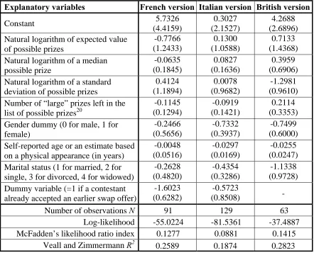
Table 5 shows that exchange decisions do not depend on the distribution of
possible monetary prizes that contestants face when the “bank” offers a swap opportunity.
Contestants, who eliminated large prizes, do not appear to be significantly more likely to
accept or reject the exchange offer compared to contestants, who eliminated small prizes.
Similarly, contestants’ decision to accept the exchange offer is apparently not affected by
expected value, median or standard deviation of prizes that are left in unopened boxes.
18
Table 5 also shows no evidence of exchange decisions being correlated with
individual-specific variables (only in the Italian version of Deal or No Deal female and
older contestants are marginally less likely to accept a swap offer). Overall, none of
lottery-specific or individual-specific variables has a significant explanatory power for
predicting the decisions to accept the exchange offer.19 Such decisions appear to be quite
random and spontaneous, perhaps indicating that contestants are indeed largely
indifferent between accepting and rejecting the swap offer.
Explanatory variables French version Italian version British version
Constant 5.7326
(4.4159)
0.3027 (2.1527)
4.2688 (2.6896) Natural logarithm of expected value
of possible prizes
-0.7766 (1.2433) 0.1300 (1.0588) 0.7133 (1.4368) Natural logarithm of a median
possible prize -0.0635 (0.1845) 0.0827 (0.1636) 0.3959 (0.6906) Natural logarithm of a standard
deviation of possible prizes
0.4124 (1.1894) 0.0078 (0.9682) -1.2981 (0.9610) Number of “large” prizes left in the
list of possible prizes20
-0.1145 (0.1294) -0.0919 (0.1421) 0.2114 (0.3353) Gender dummy (0 for male, 1 for
female) -0.2466 (0.5656) -0.7332 (0.3937) -0.7499 (0.6000) Self-reported age or an estimate based
on a physical appearance (in years)
-0.0048 (0.0516) -0.0297 (0.0169) -0.0255 (0.0247) Marital status (1 for married, 2 for
single, 3 for divorced, 4 for widowed)
-0.2628 (0.4820) -0.4354 (0.3286) -1.1338 (0.9728) Dummy variable (=1 if a contestant
already accepted an earlier swap offer)
-1.6023 (0.6282)
-0.5723
(0.8508) -
Number of observations N 91 129 63
Log-likelihood -55.0224 -81.5361 -37.4887
McFadden’s likelihood ratio index 0.1277 0.0881 0.1415
[image:22.612.84.526.265.622.2]Veall and Zimmermann R2 0.2589 0.1874 0.2823
Table 5 Estimated coefficients (standard errors) in a logit regression of exchange decisions (dependant variable is 1 if contestant swaps boxes and 0 otherwise)
19
The only variable that is statistically significant (in the French version of Deal or No Deal) is a dummy variable indicating whether a contestant already accepted a swap offer earlier in the course of the show.
20
6. Conclusion
Television show Deal or No Deal offers a unique opportunity to study individual
decision making under risk using lotteries with outcomes as high as half a million euros.
Perhaps for the first time since the famous thought experiment of Maurice Allais, we can
investigate choice between large-stake lotteries with real incentives and real people.
Contestants from various regions of France, Italy and United Kingdom are widely
dispersed in terms of age and occupation, which makes them a more diversified subject
pool compared to the undergraduate students in the conventional laboratory experiments.
Deal or No Deal contestants are endowed with a sealed box containing unknown
monetary prize (drawn from a known uniform distribution). In French, Italian and British
versions of Deal or No Deal, contestants can exchange their initial endowment for an
identical box with another prize drawn from the same uniform distribution. We find that
73% of French contestants, 47% of Italian contestants and 43% of British contestants,
who receive the possibility to swap their box, accept the exchange offer at least once.
Thus, Deal or No Deal contestants reveal weaker endowment effects compared to typical
findings in the laboratory experiments. These results suggest that even inexperienced
individuals may overcome endowment effect when facing unusual decision problem
involving substantial monetary rewards.
Exchange decisions are not correlated with lottery-specific variables such as the
expected value of possible prizes. Contestants, who eliminated large prizes from the list
of possible prizes, do not appear to be more likely to accept or reject the exchange offer.
We also find that exchange decisions are not correlated with individual-specific variables,
with the exception of Italian female and older contestants, who are marginally less likely
to accept the exchange offer. Thus, if there are individual differences in the strength of
In traditional laboratory studiesofendowment effects(e.g.PlottandZeiler(2007),
List(2004), Knetsch (1989)) subjects are endowed with physical goods of a similar value.
In contrast, Deal or No Deal contestants receive uncertain endowments. The use of risky
lotteries as the objects of exchange is a promising avenue for studying endowment effects
when stakes are as high as half a million Euros. Commodities that have similar high value
(e.g. real estate properties, Monet paintings from the same series etc.) are never exactly
identical with many small inconsequential differences (e.g. a view from the window).
An experimentercan hardlycontrol forsuch differences that maybe just sufficient
for inducing a strict preference for one of the objects. However, an experimenter can
always construct identical risky lotteries over cash prizes or physical goods. Laboratory
studies show that the effects of loss aversion are just as strong in choice under risk as they
are in a riskless choice (e.g. Tversky and Kahneman (1992)). Thus, the research on the
loss aversion and the endowment effect can benefit from further laboratory experiments
on the exchange asymmetries when the objects of exchange are identical risky lotteries.
If contestants incorporate the (initially unknown) content of the box that they
select for themselves at the beginning of the show into their reference point, loss aversion
predicts that contestants should always reject a swap offer. This is a stronger implication
of loss aversion than in the mug-candy bar exchange experiments (Knetsch and Sinden
(1984), Samuelson and Zeckhauser (1988) and Knetsch (1989)). In these experiments
loss aversion implies that the fraction of individuals, who are not willing to exchange a
mug (candy bar) for a candy bar (mug), should be higher in the treatment where subjects
were initially endowed with a mug (candy bar) compared to the fraction of subjects in the
baseline treatment, who were endowed with nothing and subsequently choose a mug
(candy bar). Such control treatment is not required in our natural experiment because two
References
Abdellaoui, M. (2000): “Parameter-Free Elicitation of Utility and Probability Weighting
Functions,” Management Science, 46, 1497-1512.
Blavatskyy, Pavlo and Ganna Pogrebna (2009) “Models of Stochastic Choice and
Decision Theories: Why Both are Important for Analyzing Decisions” Journal of
Applied Econometrics,forthcoming
Blavatskyy, Pavlo and Ganna Pogrebna (2008) “Risk Aversion When Gains Are Likely
and Unlikely: Evidence from a Natural Experiment with Large Stakes” Theory and
Decision, 64, 395-420
Bombardini, M. and F. Trebbi (2005): “Risk Aversion and Expected Utility Theory: A Field Experiment with Large and Small Stakes” unpublished manuscript
Brookshire, D., and D. Coursey (1987): “Measuring the Value of a Public Good: An
Empirical Comparison of Elicitation Procedures,” American Economic Review, 77,
554–566.
Coursey, D., J. Hovis, and W. Schulze (1987): “The Disparity Between Willingness to
Accept And Willingness to Pay Measures of Value,” Quarterly Journal of
Economics, 102, 679–690.
Charness, G. and D. Levin (2005) “When Optimal Choices Feel Wrong: A Laboratory
Study of Bayesian Updating, Complexity, and Affect” American Economic Review
95, 1300-1309
Deck, C., J. Lee and J. Reyes (2008) “Risk Attitudes in Large Stakes Gambles: Evidence
from a Game Show” Applied Economics40(1), 41-52
Friedman, D. (1998) “Monty Hall’s Three Doors: Construction and Deconstruction of a
Choice Anomaly” American Economic Review88, 933-946
Kahneman D., J. L. Knetsch, and R. H. Thaler (1990): “Experimental Tests of the
Endowment Effect and the Coase Theorem,” Journal of Political Economy, 98, 25–
48.
Kahneman D., J. Knetsch, and R. Thaler (1991): “Anomalies: The Endowment Effect,
Loss Aversion, and Status Quo Bias,” Journal of Economic Prospectives, 5(1),
193–206.
Kahneman, D., and A. Tversky (1979): “Prospect Theory: An Analysis of Decision
Under Risk,” Econometrica, 47, 263–291.
Knetsch, J. L. (1989): “The Endowment Effect and Evidence of Nonreversible
Knetsch, J. L. and J. A. Sinden (1984): “Willingness to Pay and Compensation Demanded: Expermental Evidence of an Unexpected Disparity in Measures of
Value,” Quarterly Journal of Economics, 99(3), 507–521.
Knez, P., V. L. Smith, and A. Williams (1985): “Individual Rationality, Market
Rationality, and Value Estimation,” American Economic Review, 75, 397–402.
Koszegi, B. and M. Rabin (2006) “A Model of Reference-Dependent Preferences,”
Quarterly Journal of Economics, 121(4), 1133-1165
List, J. (2004) “Neoclassical Theory Versus Prospect Theory: Evidence From the
Marketplace,” Econometrica, 72(2), 615-625.
Loomes, G. and Sugden, R. (1987) “Some applications of a more general form of regret
theory” Journal of Economic Theory41, 270-287
Myagkov, M. and Ch. R. Plott (1997) “Exchange Economies and Loss Exposure: Experiments Exploring Prospect Theory and Competitive Equilibria in Market
Environments,” American Economic Review, 87(5), 801-828.
Plott, Ch. R. and K. Zeiler (2007) “Exchange Asymmetries Incorrectly Interpreted as
Evidence of Endowment Effect Theory and Prospect Theory?" American Economic
Review97, 1449
Pogrebna, Ganna (2008) “Naive Advice When Half-a-Million is at Stake” Economics
Letters98 (2), 148-154
Post, T., M. Van den Assem, G. Baltussen and R. Thaler, (2008) "Deal or No Deal?
Decision Making Under Risk in a Large-Payoff Game Show," American Economic
Review98(1), 38-71.
Samuelson, W. and R. Zeckhauser (1988): “Status Quo Bias in Decision Making,”
Journal of Risk and Uncertainty, 1(1), 7–59.
Shogren, J.F., S.Y. Shin, D.J. Hayes and J.B. Kliebenstein (1994): “Resolving
Differences in Willingness to Pay and Willingness to Accept,” American Economic
Review, 84, 255–270.
Thaler, R. (1980): “Toward a Positive Theory of Consumer Choice,” Journal of
Economic Behavior and Organization, 1, 39–60.
Tversky, A., and D. Kahneman (1991): “Loss Aversion in Riskless Choice: A
Reference-Dependent Model,” Quarterly Journal of Economics, 106, 1039–1061.
Tversky, A. and Kahneman, D. (1992): “Advances in prospect theory: Cumulative
Figure 1 Screenshot with a List of Possible Prizes in the French version of Deal or No Deal
[image:27.612.110.500.374.655.2]0 2 4 6 8 10 Fr e q ue n c y
1 2 3 4 5 6 7 8 9 10 11 12 13 14 15 16 17 18 19 2 0
B o x n um be r 0 .0 1 E U R
0 2 4 6 8 10 Fr e que nc y
1 2 3 4 5 6 7 8 9 10 11 12 13 14 15 16 17 18 19 2 0
B o x n um be r
0.20 EUR 0 2 4 6 8 10 12 Fr e q ue nc y
1 2 3 4 5 6 7 8 9 10 11 12 13 14 15 16 17 18 19 2 0
B o x num b e r
0.50 EUR 0 2 4 6 8 10 Fr e q ue nc y
1 2 3 4 5 6 7 8 9 10 11 12 13 14 15 16 17 18 19 2 0
B o x n um be r
1 EUR 0 2 4 6 8 10 12 Fr e q ue nc y
1 2 3 4 5 6 7 8 9 10 11 12 13 14 15 16 17 18 19 2 0
B o x nu m be r
5 EUR 0 2 4 6 8 10 Fr e q ue nc y
1 2 3 4 5 6 7 8 9 10 11 12 13 14 15 16 17 18 19 2 0
B o x nu m be r
10 EUR 0 2 4 6 8 10 12 Fr e q ue nc y
1 2 3 4 5 6 7 8 9 10 11 12 13 14 15 16 17 18 19 2 0
B o x num b e r
50 EUR 0 2 4 6 8 10 F re que nc y
1 2 3 4 5 6 7 8 9 10 11 12 13 14 15 16 17 18 19 2 0
B o x number 100 EUR 0 2 4 6 8 10 Fr e que nc y
1 2 3 4 5 6 7 8 9 10 11 12 13 14 15 16 17 18 19 2 0
B o x number 250 EUR 0 2 4 6 8 10 12 14 Fr e q ue nc y
1 2 3 4 5 6 7 8 9 10 11 12 13 14 15 16 17 18 19 2 0
[image:29.612.49.582.71.632.2]B o x number 500 EUR
Figure 4 The Distribution of Prizes from 0.01 to 500 Euros Across Twenty Boxes
χ2 =21.20
p=0.3259
χ2 =16.80
p=0.6034
χ2 =23.60
p=0.2119
χ2 =13.20
p=0.8282
χ2 =20.00
p=0.3946
χ2 =25.20
p=0.1541
χ2 =32.00
p=0.0313
χ2 =15.60
p=0.6838
χ2 =17.20
p=0.5763
χ2 =34.40
0 1 2 3 4 5 6 7 8 9 F re que nc y
1 2 3 4 5 6 7 8 9 10 11 12 13 14 15 16 17 18 19 2 0
B o x number 5,000 EUR 0 1 2 3 4 5 6 7 8 9 Fr e que nc y
1 2 3 4 5 6 7 8 9 10 11 12 13 14 15 16 17 18 19 2 0
B o x number 10,000 EUR 0 1 2 3 4 5 6 7 8 Fr e que nc y
1 2 3 4 5 6 7 8 9 10 11 12 13 14 15 16 17 18 19 2 0
B o x number 15,000 EUR 0 1 2 3 4 5 6 7 8 9 Fr e q ue n c y
1 2 3 4 5 6 7 8 9 10 11 12 13 14 15 16 17 18 19 2 0
B o x number 20,000 EUR 0 2 4 6 8 10 12 Fr e q ue n c y
1 2 3 4 5 6 7 8 9 10 11 12 13 14 15 16 17 18 19 2 0
B o x number 25,000 EUR 0 1 2 3 4 5 6 7 8 9 10 Fr e q ue nc y
1 2 3 4 5 6 7 8 9 10 11 12 13 14 15 16 17 18 19 2 0
B o x number 50,000 EUR 0 2 4 6 8 10 12 Fr e q u e nc y
1 2 3 4 5 6 7 8 9 10 11 12 13 14 15 16 17 18 19 2 0
B o x number 75,000 EUR 0 1 2 3 4 5 6 7 8 9 10 Fr e q ue nc y
1 2 3 4 5 6 7 8 9 10 11 12 13 14 15 16 17 18 19 2 0
B o x number 100,000 EUR 0 2 4 6 8 10 12 F re q ue nc y
1 2 3 4 5 6 7 8 9 10 11 12 13 14 15 16 17 18 19 2 0
B o x number 250,000 EUR 0 1 2 3 4 5 6 7 8 9 Fr e que nc y
1 2 3 4 5 6 7 8 9 10 11 12 13 14 15 16 17 18 19 2 0
[image:30.612.48.586.71.634.2]B o x number 500,000 EUR
Figure 5 The Distribution of Prizes from 5,000 to 500,000 Euros Across Twenty Boxes
χ2 =22.80
p=0.2463
χ2 =12.00
p=0.8856
χ2 =10.40
p=0.9424 χ
2 =22.40
p=0.2648
χ2 =24.00 p=0.1962
χ2 =17.20
p=0.5763
χ2 =21.20
p=0.3259
χ2 =28.80
p=0.0692
χ2 =22.00
p=0.2843
χ2 =16.80