Adaptive wavelet image compression

University of Warwick institutional repository: http://go.warwick.ac.uk/wrap

A Thesis Submitted for the Degree of PhD at the University of Warwick

http://go.warwick.ac.uk/wrap/67099

This thesis is made available online and is protected by original copyright. Please scroll down to view the document itself.

Adaptive Wavelet Image Compression

Nasir Mahmood Rajpoot, M Sc.

A thesis submitted to

The University of Warwick

for the degree of

Doctor of Philosophy

Adaptive Wavelet Image Compression

Nasir Mahmood Rajpoot A thesis submitted to The University of Warwick

for the degree of Doctor of Philosophy

April 2001

In recent years, there has been an explosive increase in the amount of digital image data. The requirements for its storage. and communication can be reduced considerably by compressing the data while maintaining their visual quality. The work in this thesis is concerned with the compression of still images using fixed and adaptive wavelet transforms.

The wavelet transform is a suitable candidate for representing an image in a compression sys-tem, due to its being an efficient representation, having an inherent multiresolution nature, and possessing a self-similar structure which lends itself to efficient quantization strategies using zerotrees. The properties of wavelet transforms are studied from a compression viewpoint. A novel augmented zerotree wavelet image coding algorithm is presented whose compression performance is comparable to the best wavelet coding results published to date. It is demon-strated that a wavelet image coder performs much better on images consisting of smooth re-gions than on relatively complex images. The need thus arises to explore the wavelet bases whose time-frequency tiling is adapted to a given signal, in such a way that the resulting waveforms resemble closely those present in the signal and consequently result in a sparse representation, suitable for compression purposes.

Various issues related to a generalized wavelet basis adapted to the signal or image contents, the so-called best wavelet packet basis, and its selection are addressed. A new method for wavelet packet basis selection is presented, which aims to unite the basis selection process with quanti-zation strategy to achieve better compression performance. A general zerotree structure for any arbitrary wavelet packet basis, termed the compatible zerotree structure, is presented. The new basis selection method is applied to compatible zerotree quantization to obtain a progressive wavelet packet coder, which shows significant coding gains over its wavelet counterpart on test images of diverse nature.

Keywords:

Acknowledgements

All gratitudes are due to the Almighty who bestowed upon me the great power of will, and by whose Grace I was able to conclude this work.

This work was supported mainly by the Quaid-e-Azam scholarship of the Ministry of Education, Government of Pakistan. The research was conducted within the Image and Signal Processing Research Group of the Department of Computer Science at the University of Warwick, UK, and the Computational Mathematics Research Group of the Departments of Mathematics and Computer Science at the Yale University, USA.

I would like to thank my laboratory fellows at Warwick for their friendship and pro-viding a pleasant working environment, in particular: Guo-Huei Chen, Salim Gulam, Peter Meulemans, and Xiaoran Mo. Special thanks go to Doctor Ian Levy and Doctor Artur Sowa (Yale) for their friendship, help and extraordinary patience in response to my often stupid queries related to computing and applied mathematics.

I wish to appreciate the persistent encouragement and support of my supervisor, Pro-fessor Roland Wilson, and would like to thank him very much for his guidance through-out this project. I am greatly indebted to Professor Ronald Coifman of Yale University for his inspiring ideas and generous support, Doctor Francois Meyer of University of Colorado for inviting me to visit Yale and many motivating discussions, and Doctor Cenk Sahinalp of Case Western Reserve University for introducing me to the field of data compression and a continued collaboration.

Contents

List of Figures

List of Tables

1 Introduction and Scope of Thesis

1.1 Introduction . . .

. .

. . .

. .

. .

. . .

. .

. . .

.

. . .

1.2 Related Work . . . .

1.2.1

1.2.2

Wavelet Image Coding . . .

Wavelet Packet Image Coding

1.3 Mathematical Preliminaries . . .

1.3.1 Representation Theory .

1.3.2

1.3.3

Information Theory. . . .

Computational Complexity Notation. .

1.4 Thesis Organization . . . .

vi

xi

1

2

3

4

6

7

7

9

11

2 Image Representation for Coding

2.1 Finding a Suitable Representation

2.1.1

2.1.2

2.1.3

Applied Harmonic Analysis: A Brief Overview . .

Why Wavelets? . . . .

Wavelets and Subband Decomposition.

2.2 Transform Coding. . .

2.3 Quantization Strategies . . .

2.3.1 Vector Quantization

2.4 Entropy Coding . . . .

. .

.

. . .

.

. . .

. .

Dictionary Based Coding. . 2.4.1

2.4.2 Optimal Parsing for Dictionary Based Coding .

14

17

17

26

27

31

33

37

37

38

41

2.4.3 Statistical Entropy Coding . . . . . 43

2.4.4 Arithmetic Coding

...

44

2.5 Chapter Summary . . . . . 45

3 Fixed Wavelet Image Coding 46

3.1 Haar Wavelet Transform

.

.

. . .

.

.

.

. . .

.

. . .

46

3.2 Properties of Wavelet Coefficients . . . .

3.2.1 Statistical Properties of Wavelet Coefficients

3.3 A Simple Wavelet-Thresholding Image Coder . .

3.4 Exploiting Self-Similarities Among the Subbands

3.4.1

3.4.2

3.4.3

3.4.4

3.4.5

The Idea of a Zero-tree . . . . .

Shapiro's EZW Compression. . . .

Validating the Zerotree Hypothesis. . . .

Set Partitioning in Hierarchical Trees (SPIHT)

Augmented Zerotree Image Coder (AZIC) .

3.5 Chapter Summary . . . .

4 Adapting the Wavelet Basis

4.1 Wavelet Packets . . . .

...

4.1.1

4.1.2

4.1.3

4.1.4

Number of Possible Bases

. . .

.

. .

. . .

.

. . .

.

Frequency Ordering of the Wavelet Packets

Two-Dimensional Wavelet Packets. . .

Special Wavelet Packets

. .

.

. . .

.

.

.

. .

.

. . .

. .

.

.

.

49 55 61 64 66 67 70 70 75 87

89

90

92 99 100 102

4.3

Selecting the Best Wavelet Packet Basis

4.3.1

4.3.2

Search Methods. . . .

Choice of a Cost Function

4.4 How Good is the

Best

Basis? . . . .

4.5 A New Paradigm for Basis Selection . .

4.6

Chapter Summary . . . .

5 Progressive Wavelet Packet Image Coding

5.1 Wavelet Packets Meet Zerotrees .

5.2

Compatible Zerotree Quantization

...

5.2.1

5.2.2

5.2.3

Parenting Conflict . . . .

Rules for Generating the Compatible Zero trees

Testing the Compatible Zerotree Hypothesis. .

5.3

Analysis of the Zerotree Quantization

. . .

.

.

. . .

.

5.4

The Coder Algorithm . . . .

5.5

Experimental Results and Discussion.

105 107 109 III 116 119

120

122

125

129

131

134

135

147

148

5.6

Chapter Summary. . . . .

151

6.1

6.2

6.3

Summary and Conclusions

Limitations . . .

Future Directions

6.4 Concluding Remarks

A Rate-Distortion Characteristics of Wavelet Transform

B Comparison of the Cost Functions

C Paper Presented at IEEE DCC'99

D Paper Presented at IEEE ICIP'99

References

155

158

159

160

161

165

167

179

List of Figures

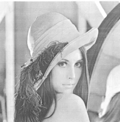
2.1 The original 512x512Lena image . . . .

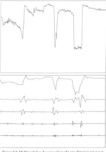
2.2 Multiresolution decomposition of a one-dimensional signal .

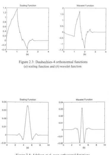
2.3 Daubechies-4 orthononnal functions . . .

. . .

.

. .

. .

. .

.

.

.

2.4 Adelson et al. near-orthogonal functions .

2.5 Daubechies et al. 9-7 biorthogonal functions . . . .

...

2.6

Discrete wavelet transfonn using a two-channel filter bank

.

...

2.7 2-d forward DWT of f(x, y) using the analysis filter bank . .

...

2.8

Subbands in the 1-level DWT of256x256 Lena . . .

2.9

2-d inverse DWT to recover

f(x,

y)

using the synthesis filter bank

..

2.10 Block diagram of a simple transform coding system . . .

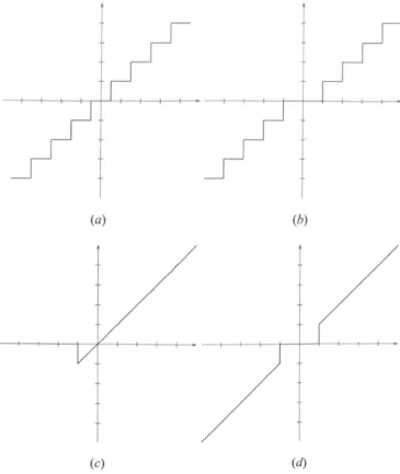
2.11 Graphs of simple scalar quantization functions.

2.12 Working of the LZ77 algorithm. . . .

2.13 Working of greedy parsing and the

FP .

22

23

24

24

25

28

30

30

31

31

35

40

3.1 Haar Functions . . . .

3.2 Gray-level histograms for the 512x512

Lena

image

47

48

3.3 Reconstruction of

Lena

from the largest 10% Haar wavelet coefficients 50

3.4 Reconstruction of

Lena

from the largest 5% Haar wavelet coefficients 51

3.5 Reconstruction ofa sine wave from Haar wavelet coefficients. 52

3.6 Decay of3-level sorted scaling coefficients

!c8[kJl

for

Lena .

3.7 Decay of3-level sorted wavelet coefficients

/cs[k]/

for

Lena.

3.8 Decay of 5-level sorted scaling coefficients

/cs[kl/

for

Lena .

57

58

59

3.9 Decay of 5-level sorted wavelet coefficients

/cs[kJl

for

Lena. .

60

3.10 Operational rate-distortion curves for a Laplacian distribution. 62

3.11 Performance of the wavelet-thresholding image coders for

Lena

65

3.12 Parent-offspring dependences in a 3-1evel DWT

3.13 Scanning order of a 3-level DWT's coefficients

. .

.

. .

.

.

.

. . . .

68

69

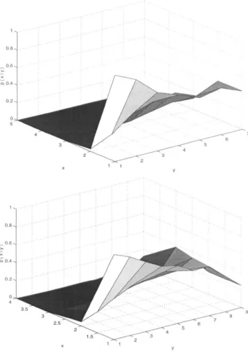
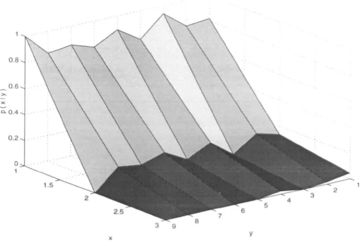
3.14 Conditional histograms for 5-level wavelet decomposition of

Lena -

I 71

3.15 Conditional histograms for 5-level wavelet decomposition of

Lena -

II 72

3.16 Conditional histograms for 5-level wavelet decomposition of

Lena -

III 76

3.17 A graphical illustration of the augmented zero trees

3.18 New scanning order for high frequency subbands .

77

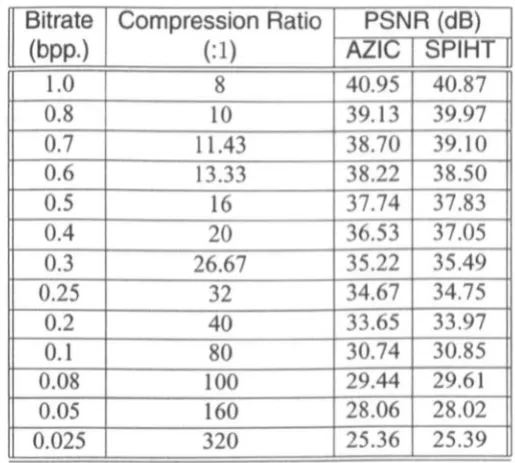
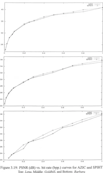
3.19 PSNR (dB) vs. bit rate (bpp.) curves for AZI C and SPIHT . . . 86

4.1 A quadratic chirp signal and its spectrogram . . . .

4.2 Full-tree wavelet packet subbands for signal in Figure 4.1

4.3 Time-frequency tilings of the quadratic chirp signal

4.4 The origina1512x512 Barbara image . . . .

93

93

94

95

4.5 Reconstruction of Barbara from the largest 5% wavelet coefficients 96

4.6 Reconstruction of Barbara from the largest 5% wavelet packet coeff-icients . . . .

4.7 Frequency-ordered Haar-Walsh wavelet packets

97

99

4.8 Fourier transform of Haar-Walsh wavelet packets in Figure 4.7 100

4.9 Frequency-ordered Daubechies-4 wavelet packets

4.10 Two-dimensional Haar-Walsh wavelet packets . .

4.11 Geometries of the best bases selected for 256 x 256 Barbara.

101

103

112

4.12 Compression numbers of the best bases selected for 256 x 256 Barbara 113

4.13 Spectrograms of quadratic chirp signal using wavelet packets . . . .. 117

5.1 Subspace tree for a 2-level wavelet decomposition . .

5.2 Split of the two-dimensional spatial frequency plane.

124

124

5.4 Subspace tree for a 3-leve1 wavelet packet decomposition .

...

127

5.5 Compatible zerotrees for a 3-level wavelet decomposition.

...

128

5.6 Parenting conflict in a wavelet packet decomposition

. .

. . . .

.

. .

130

5.7 Parent-offspring relationships for a compatible zerotree

...

130

5.8 A simple root compatible zerotree

.

. .

. . . .

. . .

. . .

.

133

5.9 The root compatible zero tree after reorganization

. . . .

. . . .

.

. .

133 5.10 Plot of the amplitude of wavelet coefficients -I

...

136

5.11 Plot of the amplitude of wavelet coefficients -II

...

136

5.12

A

sample wavelet packet geometry and the corresponding compatible zerotrees . . . . 137

5.13 Plot of the amplitude of wavelet packet coefficients -

I.

138

5.14 Plot of the amplitude of wavelet packet coefficients -II 138

5.15 Zoomed sections of Figure 5.14 . . . . 139

5.16 Joint and conditional histograms for subband numbered 3 and its

im-mediate children (binsize=80) . . . 140

5.17 Joint and conditional histograms for subband numbered 4 and its im-mediate children (binsize=50) . . . 141

5.18 Joint and conditional histograms for subband numbered 26 and its

5.19 Joint and conditional histograms for subband numbered 43 and its im-mediate children (binsize=80) . . . .

5.20 Cost of encoding the significance map vs. threshold value.

5.21 Best basis selection algorithm for zerotree quantization . .

5.22 Flowchart of the progressive wavelet packet image coding algorithm with the compatible zerotree quantization . . . .

5.23 Selected 2-d wavelet packet bases used for encoding

5.24 Portion of Barbara (table cloth) encoded at 0.25 bpp.

143

146

147

149

153

154

5.25 Portion of Fingerprints (central spiral) encoded at 0.25 bpp.. . . 154

List of Tables

3.1 Compression performance of wavelet-thresholding coding algorithms for the 512 x 512 Lena image . . . 66

3.2 Information cost of N,-Ievel wavelet coefficients for the Lena. . 67

3.3 AZIC compression results for 512 x 512 Lena image . .

85

3.4 AZIC compression results for 512 x 512 Goldhill image 87

3.5 AZIC compression results for 512 x 512 Barbara image

88

4.1 Number of possible wavelet packet bases Nd. at depth d . • . • . . •. 98

5.1 CZQ compression results for 512 x 512 Lena image . . . .

. . . .

.

.

150

5.2 CZQ compression results for 512 x 512 Goldhill image . .

. .

.

.

.

.

151

5.3 CZQ compression results for 512 x 512 Barbara image . . 152

Declaration

I declare that, except where acknowledged, the material contained in this thesis is my own work and that it has neither been previously published nor submitted elsewhere for the purpose of obtaining an academic degree.

Chapter 1

Introduction and Scope of Thesis

1.1 Introduction

The current JPEG (Joint Picture Experts Group) image coding standard [62] employs the discrete cosine transform (DeT) on 8x8 segment blocks of the image in order to de-correlate the information contained in these blocks, avoiding at the same time any global mixing of the information contained in the whole image (which is the case when the discrete Fourier transform of the whole image is taken). At low bit rates, however, this coding scheme fails to produce visually pleasing results. The blocking artifacts, in particular, are clearly visible at even medium bit rates.

A spatial frequency subband decomposition appears to be a key feature of the human visual system (HVS) [15]. Early subband image coding methods such as [12, 100] were motivated by this observation. The development of wavelets by Stromberg [78] in 1981 and the work by MalIat and Meyer [45, 46] in 1987 led to a surge of research activity in wavelet transform based image coding during the last decade or so, primar-ily due to the fact that the wavelet transform matches the main feature of the HVS mentioned above. Image coding methods based on wavelets, therefore, have become the state-of-the-art2• Zerotree quantization [73] is an effective way of exploiting the

self-similarities among high frequency subbands at various resolutions. Wavelet trans-form image coding methods based on the concept of zerotrees (groups of transtrans-form coefficients, belonging to different subbands, that are insignificant) such as [73, 71] have proved their superiority over other wavelet based methods in terms of both com-putational complexity and compression performance.

Wavelet transform based image coding methods, however, perform much better on images consisting of smooth regions with well-defined boundaries than on more

plex or textured images. Wavelet packets were invented [18] to pinpoint signal phe-nomena occurring locally in the frequency domain. The frequency adaptivity of wav-elet packets makes them capable of adaptively decomposing a given image into finer spatial frequency subbands, depending on the image contents.

Various basis selection methods [22, 67, 83] have been proposed to select the best basis 8* among a library 1) of available wavelet packet bases by using some search method and a specific cost function. The use of different cost functions may result in different

best bases which raises the issue of which is best overall. Moreover, these different

bases may produce different coding results using the same quantization method. It is, therefore, important to take into account the quantization strategy at the time of basis selection, to ensure that the basis chosen by employing a given criterion will actually result in better performance in terms of coding gains.

Apart from being efficient in terms of both computational complexity and compression performance, zerotree quantization enables the embedded (progressive) transmission and reconstruction of images, which is required in some applications. These and the better frequency localization properties of the wavelet packet transform provide reason enough to study the possible unification of wavelet packets with zerotree quantization - one of the main subjects of the work in this thesis.

1.2 Related Work

1.2.1 Wavelet Image Coding

The research work on wavelet transform image coding can be divided into two main categories: schemes which employ the idea of zerotrees in order to exploit inter-band similarities (zerotree quantization methods) and schemes which employ some other method to exploit these and other similarities and the sparseness of wavelet represen-tation.

Zerotree Quantization Methods

More precisely, a zerotree can be regarded as a quadtree consisting of a group of transform coefficients, belonging to different spatial frequency subbands, which are insignificant. The history of quadtrees (a tree whose each node, except the leaves, has four children) in image compression dates back to Wilson's work on quadtree predic-tive coding [95]. In wavelet coding, Lewis and Knowles [41] similarly hypothesized that in this tree-like structure, if the magnitude of a parent coefficient is below a given threshold, all of its children coefficients are most likely to follow this course too.

Soon after Shapiro's paper on EZW was published, an improvement was presented by Said and Pearlman [71] which gave better results by eliminating to some extent the redundancies found in an EZW-generated bitstream. In their SPIHT (set partitioning in hierarchical trees) coder, the spatial orientation trees are similar to the zerotrees of the EZW. The image coding results of SPIHT are among the best known and it is still widely regarded as a benchmark for image coding.

Non-Zerotree Quantization Methods

The

stack-run

image coder of Tsai et al. [84] achieves comparable coding results by doing a uniform scalar quantization (with a deadzone) of the wavelet transform coeff-icients, followed by a clever run-length coding which uses only four symbols for enc-oding both zero-runs and the sign and the magnitude of significant coefficients. Their run-length coding utilizes the fact that the most significant bit (MSB) of a significant coefficient does not need to be explicitly encoded if some other means of terminating the binary word can be found, and the MSB can then be used to encode the sign of the coefficient.

The Estimation-Quantization (EQ) framework of LoPresto et a1. [44] is based on mix-ture modelling of the wavelet coefficients belonging to all subbands and then finding and applying the optimal quantizers to each subband. They model the wavelet coeffici-ents as being drawn from an independent Generalized Gaussian distribution, of fixed unknown shape for each subband, having a zero mean and unknown, slowly varying variances. Based on these variance estimates, they apply an off-line rate-distortion optimized quantization strategy for each subband.

(with a 4x4 block size) to encode the lowest frequency subband, while the other sub-bands are encoded with the TCQ after distributing the bit budget optimally among all the sub bands.

1.2.2 Wavelet Packet Image Coding

Although wavelet packets offer better frequency localization, there has not been as much research activity in wavelet packet image coding as in the area of wavelet ima-ge coding, perhaps due to it being computationally more expensive than the wavelet transform. The dynamic programming approach of Coifinan and Wickerhauser [22] to select the best wavelet packet basis for a given cost function used a bottom-up search method and assumed that the cost functions were additive. Contrary to this bottom-up search for the optimal wavelet packet basis, Taswell [82, 83] advocated the use of top-down searches to obtain the so-called

near-best basis

in order to reduce the computational complexity of best basis selection, at the loss of some performance in compression.

The space-frequency quantization (SFQ) algorithm of Xiong et al. [103] employs a rate-distortion (R-D) optimization framework to select the best basis and assigns an optimal quantizer to each of the wavelet packet subbands at the same time. The best wavelet packet basis is selected using a dynamic programming approach [22] with a cost function made up of both rate and distortion.

Lapla-cian distribution and employ near optimal scalar quantizers [79] designed specifically for a memoryless Laplacian source.

The work presented here is an attempt to combine wavelet packets with zerotree quan-tization to give an efficient and flexible image compression scheme.

1.3 Mathematical Preliminaries

In this section, a brief review of the preliminary concepts from the representation and information theories, and some complexity notations are presented.

1.3.1 Representation Theory

A

vector space

over

C

or

n,

is a set

E

of vectors together with

addition

and

scalar

mUltiplication

satisfying the following for

x,

yEE and

a,

{3Ee or n:

1.

x+y

=

y+x.

2.

(x +

y)

+

z

=

x +

(y

+

z), (a{3)x

=

a{{3x).

3.

a(x

+

y)

=

ax

+

ay,

(a

+

(3)x

=

ax

+

(3x.

4. 3 DEE such that x

+

D = x, 'VxEE. 5. 3

-xEE

such that

x +

(-x)

= 0, 'VxEE. 6. 3lEE such that l·x

=

x,

'VxEE.

a). x

+

yEM, Vx, YEM.

b). aXEM, VxEM and VaEC.

An inner product of two complex-valued functions

f(t)

and

g(t)

over R is denoted by

(/, g)

and is given by

(/, g)

=

i:

j*(t)g(t)dt

(1.1)

whereas an inner product of two discrete sequences x[n] and y[n] is given by

00

(x, y) =

z:

x*[n]y[n]. (1.2)

-00

The complex (real) space

cn

(Rn) is the set of all n-tuples x

=

(Xl, ... , x

_n), with finite xiEC (R). A function

f(t)

defined on R is said to be in the Hilbert space L2(R), if

If(t)12

is Lebesgue integrable. In other words,

(1.3) In discrete tenns, a sequence x[n), nEZ is a vector in the Hilbert space [2(Z) ifit has a finite energy (Le. it has a finite square sum).

Two vectors x, yEE are called orthogonal if and only if

(x,y) =

o.

(1.4)

An orthogonal set of vectors

{Xl, X2, ... } (Xi.lXj,

Vjl-i) is called an orthonormal system if all the vectors are nonnalized to have a unit nonn. In other words,

(1.5) An orthononnal system in a vector space E is an orthonormal basis if it completely spans E. For an orthononnal system of vectors

{Xk}

in E, Bessel's inequality

IlyI12~Z:I(Xk,y)12 (1.6)

k

1.3.2 Information Theory

Consider a discrete random variable X drawing values from an alphabet

A

which is generated by a source. The probability mass function p( x)

=

Pr{ X

=

x}, where xEA, is a mapping from the symbols in A to real numbers such that the following

probability axioms are satisfied:

1. p(x)~O for any symbol

x.

2. p(A)

=

1.

3.

p(XUy)

=

p(x)

+

p(y)

for any mutually exclusive symbols

x,

YEA.

The entropy H of this random variable X is defined as

H(X) = -

L p(x) logp(x).

(1.7)

:rEA

The entropy H(X) can be referred to as the measure of information contained in the random variable, or sometimes known as the self-information of a random variable.

The unit of entropy is nats if the base of logarithm is e and it is bits if the base of

logarithm is 2, which will be used in this thesis. The lossless source coding3 theorem of Shannon [72] states that the average coding length of

X

is bounded below by

H(X).

The conditional probability

p(Ylx)

=

Pr(Y =

ylX

=

x)

is defined as the probability of another random variable

Y

taking on the value y (pos-sibly from another alphabet 8) given the random variable X takes the value

x.

Let

{Xk}

k=l, ... ,n be a partition of A. According to the total probability theorem, n

p(y)

=

LP(ylxk),p(Xk)'

(1.8)

k=l

The conditional entropy of another random variable Y given X is

H(YIX)

-

- LH(YIX=x) (1.9)

xEA

-

- L p(x) L p(ylx) logp(Ylx) (1.10)

xEA yEB

H(YIX)

-

- L L p(x, y) logp(ylx). (1.11)

xEAyEB

This defines the conditional entropy of Y given X as the expected value of the en-tropies of the conditional distributions. The joint entropy of two random variables X and

Y

with a joint distributionp(x, y) is defined as

H(X, Y) = -

2: 2:

p(x,

y)

logp(x,

y).

(1.12)

xEAyEB

The conditional and joint entropies defined above are related to each other by the chain rule as follows

H(X, Y)

=

H(X)

+

H(YIX). (1.13)

This means essentially that the joint entropy of two random variables is the sum of ent-ropy of one and the conditional entent-ropy of the other. The relative entropy or

Kullback-Leiber distance between two probability mass functions

p(

x)

and

q(

x)

is defined as D(pllq)

=

2:

p(x)log p((X)).

xEA q x

(1.14) The mutual information between X and Y is defined as the relative entropy between

the joint distribution p(x,

y)

and the product distribution p(x)p(y) " p(x,

y)

I(Xi Y) = -

L

L...J p(x, y) log (x) ( ).

xEAyEB P P Y

(1.15) The relationships between mutual information and the conditional and joint entropies are as follows

I(XjY)

_-

H(Y) - H(YIX) (1.16)

I(X;Y)

-

H(X) - H(XIY) (1.17)

It can be easily proved that the relative entropy (1.14) is a non-negative measure,

I(X;Y)~O. (1.19)

Combining (1.16) and (1.19), we get

H(Y/X)::;H(Y) (1.20)

with equality if and only if X and Y are independent. Intuitively, this means that knowing another random variable

Y

can only reduce, on the average, the uncertainty

in

X.

This important result will be used later in this thesis to efficiently encode the transform coefficients belonging to different subbands.

1.3.3 Computational Complexity Notation

Consider a function g(n). The three most commonly used complexity notations work as a mapping from a function g(n) to a set of functions. The 8-notation defined as

e

(g(n))

=

{f(n) :

3 C},

C2, no

such that 0::;

clg(n) ::; f(n) :::; c2g(n),

V n~no}

(1.21)

bounds a function to within constant factors. The O-notation defined as

o

(g(n))

=

{f(n) :

3 C and

no

such that 0::;

f(n)::; cg(n),

Vn~no}

(1.22)

gives an upper bound for a function to within a constant factor. The o'-notation defined as

n

(g(n))

=

{f(n) :

3 c and

no

such that 0::;

cg(n) ::; f(n),

V n~no}

(1.23)

1.4 Thesis Organization

In this thesis, a detailed study of the theoretical and practical aspects of a wavelet approach - in its general adaptive fonn - to the image coding problem is carried out.

Issues related to the image representation in a transfonn coding framework are dis-cussed in the next chapter. The quest for a suitable representation starts with a brief overview of applied harmonic analysis. The wavelet transfonn is selected as a suitable candidate for image representation, followed by an explanation of the wavelet subband decomposition of images using filter banks. Two other components of the transfonn coding framework, quantization and entropy coding, are also discussed. Entropy cod-ing methods are classified into two main categories: dictionary based entropy coders and statistical entropy coders. A new improvement of the well known Ziv-Lempel dictionary compression scheme is presented.

Chapter 3 builds on the arguments from the previous chapter to study the properties of the wavelet transfonn for compression purposes, in order to develop efficient wav-elet image coding algorithms. It is argued that the decay of wavelet coefficients is directly related to the compression perfonnance at various bit rates. A simple wavelet-thresholding image coder exhibits the potential gains that can be obtained by employ-ing a more sophisticated quantization strategy. The idea of zero tree quantization is explained and an improved coding algorithm is presented, whose compression perfor-mance is comparable to the state-of-the-art.

of available wavelet packet bases are discussed. Necessary and sufficient conditions for a basis selected using one cost function to be better than another basis selected using a different cost function are presented. A new paradigm for wavelet packet basis selection which emphasizes the role of quantization strategy is presented.

Chapter 5 starts with the presentation of a general zerotree quantization framework for the wavelet packet transfonn. A set of rules is defined to construct the

compati-ble zero trees for an arbitrary wavelet packet basis. The wavelet packet subbands are modelled as a Markov chain in order to efficiently estimate the cost of zerotree quan-tization. This estimation is used to select the best wavelet packet basis, in the spirit of the new paradigm presented in the previous chapter. A progressive wavelet pack-et coder combining this cost estimator with the new compatible zerotree quantization gives significant coding gains, O.6-1.5dB for the

Barbara

image, compared with its wavelet counterpart.

Chapter 2

Image Representation for Coding

Many people find it useful to take notes of the seminars or meetings that they attend. We all know that musical scores are capable of describing a symphony, with reproduc-tion of the symphony being dependent on the interpretareproduc-tion by musicians. Similarly, mathematical symbols and equations are helpful in explaining certain concepts and representing various natural phenomena. These are all familiar examples of a repre-sentation. What is representation and why do we need it? The Concise Oxford

Dictio-nary defines 'representation' as an image, likeness, or reproduction of a thing, e.g. a

painting or drawing. In his famous book Vision [51], Marr defines 'representation' in somewhat recursive terms as

"a formal system for making explicit certain entities or types of informa-tion, together with a specification of how the system does this. And I shall call the result of using a representation to describe a given entity a de-scription of the entity in that representation."

the event, we can reconstruct in our minds the whole event in a relatively easier way. These notes are, in a sense, a compressed version of the seminar: they highlight what was talked about. How easily they can recapitulate the whole event and how much of the information they are capable of reproducing clearly varies from one set of notes to anotherl. They are, nevertheless, a representation which briefly describes the seminar highlights.

The ease of reconstruction, the resources required to describe what is being represent-ed, and the loss of information after reconstruction all depend largely on one thing: the language chosen for representation. As renowned harmonic analyst Yves Meyer says [35]:

"Different languages have different strengths and weaknesses. French is effective for analyzing things, for precision, but bad for poetry and con-veying emotion - perhaps that

s

why the French like mathematics so much. I'm told by friends who speak Hebrew that it is much more expressive of

poetic images. So

if

we have information, we need to think, is it best expressed in French? Hebrew? English? The Lapps have 15 different wo-rds for snow, so

if

you wanted to talk about snow, that would be a good choice."

Natural images, in their raw form, are not suitably represented for their redundancies to be exploited for coding purposes. Thus arises the need for representing or transcribing

the image into another domain (or language). In other words, a 'sparse' representa-tion is required which can make the image redundancies more easily exploitable using structural and/or statistical approaches, thus reducing the number of bits required to

encode the image. An invertible representation incurs no loss of information, i.e. the image can be exactly reconstructed. The image representation can, however, be enc-oded with fewer bits, introducing some loss of information. The transcription and encoding should be carried out in such a way that the loss of information is minimal and the perceived quality of the decoded image is close to the original image.

The human visual system (HVS) responds more to the edge information (or the high bandwidth contents) in an image than the smooth information (or the low frequency contents) [51]. Human viewers notice distortion in smooth areas more easily than near the edges, the so-called masking effect [32]. Masking experiments show that we notice distortion in the same band as the local signal less than out-of-the-band noise [16, 77]. It seems that the HVS does a form of frequency decomposition using Gabor wavelets [94]. In order to reproduce a visually pleasing (or psychovisually tuned) image, a sparse representation that can perform a similar kind of channel or subband decomposition would be an ideal choice. The Fourier transform, introduced by Fourier in 1807, is an extremely useful analysis tool that reveals the frequency information contained in a signal. The continuous Fourier transform

FI(w)

of a function

f(t)

is given by

+00

FI(w)

=

f

f(t)

e-

iwt

dt.

(2.1)

-00

The original function

f

(t)

can be reconstructed from

FI

(w)

by taking the inverse trans-form as follows

+00

f(t)

=

~

/

FI(w) e

iwt

dt.

211"

-00

(2.2)

are non-stationary in nature and their representation in the Fourier domain makes it difficult to analyze and reproduce its local properties due to the global mixing of

in-formation by the Fourier transform [47]. Moreover, real-world signals are generally aperiodic and finite. This causes the induction of artificial oscillations (also known as the Gibbs phenomenon [9, 60]) near signal discontinuities due to truncation of the high

frequency terms. The application of Heisenberg's uncertainty principle to image

pro-cessing (97) suggests that when dealing with problems in image propro-cessing, analysis

and coding, there is always a localization trade-off between space and spatial frequen-cy. In the next section, we discuss alternatives to the Fourier transform which provide both space and frequency localization.

2.1 Finding a Suitable Representation

Harmonic analysis, the study of harmonic components of a given signal, has had an

enormous impact on the evolution of present day image coding techniques (for a de-tailed exposition on the topic, see [27]). We attempt to present a very brief review of applied harmonic analysis only from the viewpoint of representation for coding purposes. Wavelet transforms are then selected as a starting point for efficient image representation in a compression framework.

2.1.1 Applied Harmonic Analysis: A Brief Overview

The decomposition of a signal into waveforms having a finite spread in the time-frequency plane sounds like a reasonable thing to do in order to extract useful frequen-cy contents of the signal while avoiding the global mixing of information. Wigner, a

as follows

+00

W{t,

e)

=

I

f{t +

~)J(t

-

~) e-i~tdT.

(2.3)

-00

Waveforms having compact support in both time and frequency were termed as

ele-mentary time-frequency atoms by Gabor in 1946 [29]. He argued that decomposing a signal over these elementary time-frequency atoms is closely related to our perception of sounds. The closely related windowed Fourier transform (WFT)

FG(S,

e)

of the signal

f

(t) is defined as

+00

FG(s,e)

=

!

f(t) 9s,dt)dt

(2.4)

-00

where

(2.5) is a time window. In 1948, Ville [86] rediscovered and generalized the notion of time-frequency energy function similar to the Wigner distribution discussed above (to be termed later as Wigner-Ville distribution).

Although the WFT or short-term Fourier transform (STFT) provides a localized time-frequency representation, it brings with it the properties of the Fourier transform in each locality. Consider, for example, the time-frequency tiling of the STFT of an impulse, which encompasses all possible frequencies, however well localized in time it may be. Moreover, the global mix of information is now replaced by the local mix of information. This local mix and the discontinuity of basis functions at the block boundaries are largely responsible for the blocky artifacts caused by the JPEG image compression standard [62] at low bit rates. The JPEG standard employs block-based discrete cosine transform or DCT [2] for decorrelating the blocked image data2•

As Daubechies proves in [25], there are no 'good' orthogonal bases in the case of the STFT due to its limited localization properties in both time and frequency. The

local cosine bases

[91,49, 19] were designed to provide efficient time (space) local-ization for signal (image) analysis purposes. These bases (termed as the

Malvar bases

by Coifman and Meyer) are obtained by multiplying smooth windows of successive finite time intervals (which may be of different length) with local cosine functions of different frequencies given by

(2.6)

where lp

=

ap+l - ap is the size of each interval rap, ap+d and

g(t)

is the indicator function

t _

{I

ifO~t<l

g( ) -

0 otherwise. (2.7)

The local cosine basis is well adapted for signals whose properties may vary in time but which do not include structures of very different time and frequency spread at any given time [47]. A

best

local cosine basis is an efficient representation if the image does not include very different frequency structures in the same region. In other words, it offers good localization in time at the cost oflosing flexibility in frequency adaptation in each locality.

Wavelet Transform

behind wavelets is that shifts and dilations of a prototype function

'I/J(t)

are chosen instead of its shifts and modulations. The function

'I/J(t)

satisfies

+00

!

'I/J(t) dt

=

0 (2.8)

-00

and is also called mother wavelet. When this function is dilated by a factor of a and translated by another scalar b, we get another wavelet denoted by 'l/Jab(t) and given by (2.9)

The wavelet transform

Fw{a, b)

of a function

J(t)

at a scale a and position

b

is com-puted by correlating

J

with the wavelet 'l/Jab(t)

1 +00

(t -

b)

Fw(a, b)

=

Va

!

'I/J

-a- f(t)dt.

-00

(2.10)

When a scale of2j is used, (2.9) can be written as,

(2.11)

where a

=

2; and b

=

2; k. These wavelet bases dyadically decompose the function

J(t)

into pieces belonging to different subspaces. The subspaces are of two types: the scaling space

Yj

and the wavelet space Wj • The subspace

Yj

is spanned by the basis { c!>; (t - 2j

k) }

kez and the subspace Wj is spanned by the basis {'l/Jj

(t -

2j

k) }

keZ,

where

¢j(t)

=

2-j/2c!>(2-

j t), 'l/Jj(t)

=

2-j/

2

'I/J(2-j t). ¢(t)

is the scaling function, which is used to compute the approximation of

J(t)

at different scales, and

'I/J(t)

is the mother wavelet function, used to determine the difference or detail information. This decomposition is such that,

(2.12)

The subspace Wj corresponds to the detail at level j. Together, the space V+oo and

can represent an arbitrary function

f(t)

from L2(n). This is illustrated in Figure 2.2, which shows the 4-level multiresolution decomposition of a I-dimensional discrete signal (a vector made from the 325th column of the 5I2x5I2

Lena

image shown in Figure 2.1, going through the hat, the left eye, and down the shoulder). The signal components shown here correspond to the subspaces

V-

6 ,

W-

6,

W-

7 ,

W-

8, and

W-

9

in order from top to bottom. Some commonly used scaling and wavelet functions are shown in Figures 2.3,2.4 and 2.5.

The wavelet transform is particularly good at highlighting the high frequency signal contents at multiple scales. This becomes clear when one considers the wavelet trans-form of an impulse. The higher the bandwidth of a wavelet function, the more compact support it has in time and thus more capable it is of providing localized information about the impulse (unlike the STFT, where time support remains the same for all fre-quencies in a given time window). This helps one to pinpoint exactly where in time the impulse is occurring.

Wavelet Packet Transform

A more general form of the wavelet basis, known as the

wavelet packet basis

[18, 20] is constructed by adaptively segmenting the frequency axis (as opposed to the adap-tive segmentation of time axis in case of local cosine basis). The frequency intervals of varying bandwidths are adaptively selected to extract specific frequency contents present in the given signal. This frequency segmentation is useful, for example, to analyze a local phenomenon occurring in the signal and belonging to a specific fre-quency band.

[image:38.503.41.450.156.569.2]

[image:39.500.65.423.114.627.2]

Figure 2.2: Multiresolution decomposition of a one-dimensional signal

Scaling Function Wavelet Function

1.4 r---,---,--~--__, 2r---,--~--~--_,

1.2

0.2

o

-0.2

0.5

0

-0.5

-1 -0.4 '---~----'--~----' _-1.5

o

0.04

0.03

0.02

0.01

0

-0.01 0

2 3 4 0 2

(a) (b)

Figure 2.3: Daubechies-4 orthonormal functions (a) scaling function and (b) wavelet function

Scaling Function Wavelet Function

0.04

0.03

0.02

0.01

0

-0.01

-0.02

2 4 6 8 10 0 2 4 6

[image:40.502.66.435.102.623.2]

(a) (b)

Figure 2.4: Adelson et al. near-orthogonal functions (a) scaling function and (b) wavelet function

3 4

0.05

0.04

0.03

0.02

0.01

0

-0.01 0

Scaling Function Wavelet Function

0.04

0.03

0.02

0.01

0

-0.01

-0.02

-0.03

2 4 6 8 10 0 2 4 6

(a) (b)

Figure 2.5: Daubechies et al. 9-7 biorthogonal functions

(a) scaling function and (b) wavelet function

8 10

'I/J;

(t

-

2j_{k) basis, where 'l/J°(t)}

₌

_{¢(t) and 1jJl(t)}

₌

_{1jJ(t). As opposed to the wavelet}

transfonn, which decomposes the subspace

VJ

only into

VJ+l

and

Wj+l,

the wavelet

packet transform decomposes each subspace

WJ

into W}!l and W}!tl using scaling

and mother wavelet functions respectively. Since this library of available bases

pro-vides an overcomplete description of the function

f

(t),

a fast optimization algorithm

such as [22] is required to select a combination of bases from this library which is well

suited to the function under consideration.

Related Transforms

Other recent advances in applied harmonic analysis include the development of the

multi resolution Fourier transform (MFT) [96], brushlets [57], and adaptive

time-fre-quency tiling [34]. Although each of these transforms is quite useful to represent

images for analysis purposes, we do not find any of them a particularly suitable

can-didate for image representation in compression systems: the MFT due to its lack of

lirnit-ed applicability, and the adaptive time-frequency tiling due to its high computational complexity.

2.1.2 Why Wavelets?

We select the wavelet transfonn, to start with, as a representation language in an image coding framework for the following reasons:

a) Sparse Representation: Although the overall variance is preserved by the wavelet decomposition of a given image into low and high frequency subbands [II], it is the distribution of coefficients that detennines how efficient the decomposition is from a coding viewpoint. The wavelet transfonn provides a sparse representation, with trans-fonn coefficients corresponding to smooth regions being very small, as is illustrated in the next section. This makes the wavelet transfonn particularly suitable for compress-ing images with smooth regions.

b) Multiresolution Decomposition: A multiscale representation is ideal, given the fact that there is no natural scale for images. The multiresolution nature of a wavelet de-composition brings with it multi scale edge detection [48] which can be used to effi-ciently reconstruct an image (according to Marr's conjecture [51]).

c) Self-Similarity: Despite being sparse, the wavelet subbands exhibit structural redun-dancies and can be organized in a tree structure. Moreover, the wavelet transfonn has a self-similar kind of structure due to its multiscale nature and orientation selectivity, which can be exploited for coding purposes [93, 40].

bound-ed variation [47].

2.1.3 Wavelets and Subband Decomposition

Let

f(t)EL2(R)

denote a continuous signal. It is desired to find a complete orthonor-mal basis which spans

L2(R).

Let

'Ij;(t)

denote the mother wavelet function, so that the basis functions in

{'Ij;jk}

are the scaled and translated versions

of'lj;(t)

given by (2.11). The signal

f(t),

when represented in the wavelet domain, can be written as,

f(t)

=

L L

Cjk'lj;jk(t)

(2.13)

j k

where

Cjk

=

(f(t), 'lj;jk(t)).

(2.14)

The wavelet transfonn of a digital image can be computed with the help of filter banks, as described in the following pages.

Filter Banks

In order to compute the multiresolution wavelet decomposition of the discrete-time signals, filter banks are used. In a two-channel filter bank, as shown in Figure 2.6, there are two filters on each side. The lowpass filter H and the highpass filter G correspond to the scaling function

¢(t)

and the wavelet function

'Ij;(t)

respectively in the continuous time. These filters separate the signal into frequency subbands. To avoid the redundancy of the outputs of H and G, both the outputs U o and Ul are

downsarnpled by a factor of 2, the operation denoted by

(..j.

2). This constitutes the

Figure 2.6: Discrete wavelet transform using a two-channel filter bank

H = HT and G = G T, that is to say that the synthesis bank filters are the time reverse

of those in the analysis bank.

Ideally, the approximated signal x( n) should be exactly the same as the original

in-put signal x(n): the reconstruction should be perfect. But there is a problem: the

downsampling operation is a linear but time-variant operation and is responsible for

the possible aliasing introduced in the frequency spectrum of the downsampled signal,

due to the presence of a X

(w

+

7r)

term, where X

(w)

denotes the Fourier transform of

the signal x(n). Croisier et al. [23] showed, in 1976, that the input signal x(n) can be

recovered from the filtered and subsampled signals by using a special class of filters

called quadrature mirror (QM) filters to cancel the aliasing terms. This is possible

if X(w) is band-limited to either the upper half-band or the lower half-band [24], the

so-called spectral factorization.

Subband Decomposition

The analysis side of a two-channel filter bank (discussed above) can be used to

com-pute the multiresolution wavelet decomposition of an image. What is required now is

a simple and fast method for the computation of wavelet transform coefficients of an

wavelet transform (DWT) can be computed using a conjugate quadrature filter (CQF) pair

h[n]

and

g[n]

as follows,

and

ci[n]

=

Lh[k]c

i-

1

_{[2n -}

_k]

Ie

If[n]

=

L

g[k]c

i

- 1

[2n - k],

k

(2.15)

(2.16)

where

cOrn]

=

x[n]

represents the original signal and

ci[n], £ii[n],

i

=

1,2, ... are the scaling and wavelet coefficients respectively. In a CQF pair,

g[n]

=

(-I)nh[I -

n].

The simplest extension of the DWT to two-dimensions (2-d) is the separable DWT. The I-d DWT is performed on the rows (treating each of them as a I-d signal) fol-lowed by a I-d DWT on the columns, as shown in Figure 2.7. The order does not matter here. This 2-d DWT splits an image of size m x n into four subimages, each of size

r;

x ~. These four subimages represent the frequency information as in Figure 2.8, which shows a I-level DWT of Lena, and are called subbands. Note that the three high

frequency subbands were rescaled in order to improve the visibility. The subband LL represents the lowest frequency components of the original image at a coarse scale. The remaining three subbands HL, LH, and HH represent the high frequency compo-nents, especially the edges, of the image at a coarse scale. A closer look at these three

I

H(y)

~

(.). 2) In I y direction

hd.r:, y) h(x,y)

M

H(x)

~

(.). 2) ,n x direction

hll(x fix,y)

I

G(y)

~

(.). 2) In

I y dlrccllon

, y)

-I

H(y)

I-(.). 2) ,n

I y dlfC~clion

IlId.£ , V)

G(x)

I-

;It (.). 2) direction '"

III (z, 1/)

I

G(y)

J-

(.j.

2) 'n 11111 (x,

L y dlreclion

V)

Figure 2,7: 2-d forward DWT of

f(x,

y)

u ing the analysis filter bank

LL

Low frequency contents. at n coarser

scale

LH High frequency contents, in venacal

direction

HL

High frequency contents. in honzonlal cireclion

HlJ

High frequency COl1lcnts, 111 d,ugonal cireclion

!Ldx,y) _{(t 2) in}

y du"Cction

(t 2) in

x direction

!LH(X,y) _{(t 2) in}

y direcllon _f(x,y)

+

fHdx,y) _{(t 2) in}

y direction

(t 2) in

x direction

!HH(X,y) _{(t 2) in} y direclion

Figure 2.9: 2-d inverse DWT to recover f(x, y) using the synthesis filter bank

DlCOmlllNtI Q ••• 1I:Id

IIII"",~(J/tl

Im"ge Transform CMJllck,.IS Qllunt/UII/on IlIillet'J _{Entropy Coding} 80<1>11,4811$

""

.

..

F X-TF X Y-Q(X) Y of Y

Figure 2.10: Block diagram of a simple transform coding system

2.2

Transform

Coding

Once an efficient representation language has been found to transcribe a given image

into the transform domain, it is now time to introduce other components of the coding

system, The block diagram of a compression system based on the transform coding

paradigm is shown in Figure 2.10. Consider an image F which is to be encoded, In

this model, F is first transcribed into the transform coefficients X by applying the

transform T so that X = TF. The transform coefficients X are then quantized into Y

as follows

Y

=

Q(X)

=

Q(TF) (2.17)

where Q(.) denotes the quantizer function, designed so as to reduce the number of bits

responsible for the loss of information or distortion. The quantization indices Y are

then encoded (losslessly) using an entropy coding scheme, such as Huffinan coding [36], arithmetic coding [99], or dictionary coding [53]. No information is lost dur-ing entropy coddur-ing and the decoder should be able to reconstruct exactly the same quantization indices. These indices are then dequantized to approximate the transform coefficients

X,

so that

(2.18)

where Q-l denotes the dequantizer function. The decoded image

F

is now recon-structed by taking the inverse transform F = T-1

_{X where}

_T-1 _{denotes the inverse}

transform. The decoded image F is a distorted version of the original image

F,

the amount of distortion depending on the number of bits used to encode

F.

The most commonly used distortion measure is the mean-squared-error (MSE) given by

(2.19)

where

E {}

denotes the expected value function and is approximated by the following sample average

1 ( A

)2

AfSE

= -

~ F,.. - F,.. MN ~ '3 '3

I.J

(2.20)

for an image of size M x N. A related fidelity criterion, which is often used to compare the performance of image coders, is the peak-signal-to-rms-noise-ratio (PSNR) given by

PSNR

= 2010g10

(~)

(2.21)

2.3 Quantization Strategies

Quantization can be defined as a mapping Q from an input set X to an output set C such that the ordinality (number of elements) ofC is smaller than that of X. By its very nature, quantization is a non-invertible function. It maps the input x = {Xi}, XiEX, to an output q E C, where q is a quantization index taken from the set of quantization indices C. If x contains only one element, then this operation is called

scalar quantization and it is called vector quantization if

x

contains more than one elements. Dequantization is an 'inverse' operation which maps each element of C to one or more elements belonging to Y, a set consisting of the reconstruction values for the elements of X. Let the ordinality of both X and Y be N and the ordinality of

C

be

M.

Since

At 5:.N

and each disjoint subset consisting of one or more elements of X is mapped by Q to exactly one element in C, it is impossible to reverse the quantization operation by applying

Q-l.

Some authors define quantization as

Q-l

(Q).

We find the separation of Q and

Q-l

to be more convenient for a general description of quantization strategies.

The operations of rounding, truncation, and thresholding are perhaps the simplest com-monly used scalar quantization techniques. These functions are defined as follows.

Rounding function

')'(x)

returns the nearest integer to its argument

x.

')'(x) = argmin

Ix - yl

(2.22)

IIEZ

Truncation function

T(X)

returns only the integer part of its argument

x.

T(X)

=

lxJ

(2.23)

returns 0 otherwise.

e(X)

=

x lx~8 (2.24)

If x has a zero mean, an absolute thresholding function is normally used defined as, (2.25) The output ofe or 8a may usually be rounded to the nearest integer in order to reduce

the ordinality of C.

If any of these four functions is employed as a quantizer, the dequantizer Q-l is simply a straight-line function Q-l(y) = y. The graphs of these functions used as quantiz-ers are shown in Figure 2.11. The truncation function

rex)

behaves as a deadzone quantizer, since the length of interval for which rex) = 0 is twice the length of all other intervals for which

r(x)#O.

Such quantizers are of great importance for both speech and image coding because they produce a zero output for small input values. A coupling of

8

a with a scaled version of"( will produce a similar kind of result.

In general, a scalar quantizer

Q,

divides

X

into disjoint intervals ~ = (Xi-b

Xi],

1:5 i:5 AI, such that

QB(X)

= i, if xe(Xi-l,

Xi]'

The difference ~i

=

Xi - Xi-l is the length of the ith interval (Xi-I, Xi] and is also

known as the step size or the bin size of the ith quantization bin.

(a) (b)

[image:51.503.66.431.143.576.2]

(c) (d)

Figure 2.11: Graphs of simple scalar quantization functions

(a) Rounding function, (b) Truncation function, (c) Thresholding function (0 = - 1), and (d)

In a non-unifonn scalar quantizer, the step sizes ~i are not the same for all granular regions. In other words, the

boundary points

Xi are not equally-spaced. The distortion D for a non-unifonn scalar quantizer at a high resolution r is given by [30],

where

1 M

D~12~(pi~n

~

=

Pr

(XE~)

=

r

i

Ix(x)dx

=

li~i

/1:;-1

(2.26)

and

Ix(x)

is the pdf for

X

which is equal to

Ii

for XE~ if the resolution is high enough.

The two optimality conditions for a scalar quantizer

Q

8 and dequantizer

Q;\

also

known as the

nearest-neighbour condition

and the

centroid condition

respectively, are as follows.

Nearest-Neighbour Condition:

Q(x)

=

i if and only if d(x, Yi)~d(x,

Yj),

Vj-::j;i (2.27) or

Yi-l

+

Yi Xi-l = 2 •

Centroid Condition:

Q-l(i)

=

Yi

=

centroid(~)

=

argmin E{d(X,Y)IXE~}.

I/EZ (2.28)

If the distortion function

d(.,.)

in (2.28) is MSE, then

Yi

is the center of mass of the interval ~ and if it is MAE, then Yi is the median of ~.

2.3.1 Vector Quantization

A quantization function Qv that maps each vector XiEX to an index iEG is called a vector quantizer. The quantization function

Q;/

maps each iEG to a decoded vector

YiEY

The idea here is to represent a group of input values, in the fOIm of a vector, by a quantization index which can later be used to estimate these input values. This is a generalization of the scalar quantization and seems to offer more compression than a scalar quantizer Q 8 due to the representation of a group of inputs by a single index.

The nearest-neighbour and centroid optimality conditions can easily be generalized [42] so as to use the Lloyd's algorithm for finding the ~ 's and the codebook

G

whose each index is now mapped by the dequantizer

Q;;1

to a vector Yi.

The idea of zero tree quantization has recently been shown to be quite successful in the image coding domain. It can be regarded as a variable-size vector quantization scheme. A zero tree quantization index is generated when a group of input values belonging to different wavelet subbands follows a certain criterion. We shall study this quantization method in detail in later chapters.

2.4 Entropy Coding

approx-imation of the original image. This uniquely decodable lossless encoding of quantizer indices is also known as entropy coding, because lossless encoding methods are now available which can encode these indices to a bit rate close to the entropy. Let ~ denote a constant size alphabet.

An

entropy coding algorithm C reads input array T, consist-ing of

n

symbols chosen from ~, and computes an output

T'

whose representation is smaller than that of T, such that a corresponding decompression algorithm C+- can take T' as input and reconstruct T. Let T[i] denote the ith element ofT (1 ~ i ~ n), and T[i :

j]

be the subarray which begins at T[i] and ends at T[j] and so T

=

T[l : n].

There are two main types of redundancies found in data to be encoded in a reversible manner: structural and statistical. Coders based on dictionaries of common phrases are good at dealing with the former type of redundancies, while statistical coders take advantage of redundancies of the latter type. All dictionary schemes have an equival-ent statistical scheme that achieves exactly the same compression [6], but this comes with an added computational complexity, in order to accommodate all possible com-binations for the context.

2.4.1 Dictionary Based Coding

The most common compression algorithms in practice are the dictionary schemes, also called parsing [6] or textual substitution [76] schemes. Such algorithms are based on maintaining a dictionary of strings of input symbols that are called phrases, and replacing substrings of an input with pointers to identical phrases in the dictionary. The term string here refers to an array of input symbols chosen from ~ and arranged in a particular order, and the term substring refers to a sub array of the string, usually referring to the text input. The task of partitioning the input into phrases is called