A wave driver theory for vortical waves propagating across junctions with application to those between rigid and compliant walls

University of Warwick institutional repository: http://go.warwick.ac.uk/wrap

This paper is made available online in accordance with

publisher policies. Please scroll down to view the document

itself. Please refer to the repository record for this item and our

policy information available from the repository home page for

further information.

To see the final version of this paper please visit the publisher’s website.

Access to the published version may require a subscription.

Author(s): P. K. SEN, P. W. CARPENTER, S. HEGDE and C. DAVIES

Article Title: A wave driver theory for vortical waves propagating across

junctions with application to those between rigid and compliant walls

Year of publication: 2009

Link to published version:

doi:10.1017/S0022112008005545 Printed in the United Kingdom

A wave driver theory for vortical waves

propagating across junctions with application to

those between rigid and compliant walls

P. K. S E N1_{†, P. W. C A R P E N T E R}2_{‡, S. H E G D E}1

A N D C. D A V I E S3

1_{Department of Applied Mechanics, Indian Institute of Technology, New Delhi 110016, India}

2_{School of Engineering, University of Warwick, Coventry CV4 7AL, UK}

3_{School of Mathematics, Cardiff University, Cardiff CF24 4YH, UK}

(Received31 July 2007 and in revised form 19 November 2008)

A theory is described for propagation of vortical waves across alternate rigid and compliant panels. The structure in the fluid side at the junction of panels is a highly vortical narrow viscous structure which is idealized as a wave driver. The wave driver is modelled as a ‘half source cum half sink’. The incoming wave terminates into this structure and the outgoing wave emanates from it. The model is described by half Fourier–Laplace transforms respectively for the upstream and downstream sides of the junction. The cases below cutoff and above cutoff frequencies are studied. The theory completely reproduces the direct numerical simulation results of Davies & Carpenter (J. Fluid Mech., vol. 335, 1997, p. 361). Particularly, the jumps across the junction in the kinetic energy integral, the vorticity integral and other related quantities as obtained in the work of Davies & Carpenter are completely reproduced. Also, some important new concepts emerge, notable amongst which is the concept of the pseudo group velocity.

1. Introduction

Waves incident on a junction between two different wave-bearing media are commonly met in many practical applications. In many cases well-established techniques exist for calculating the transmitted, reflected and diffracted waves in terms of the incident wave at the junction (Lighthill 1978; Billingham & King 2000). But no suitable method appears to have been developed for calculating the amplitude of the transmitted wave when a rotational (vortical) wave in a fluid is incident on a junction with a different wave-bearing system. Here we present a novel method for solving such problems.

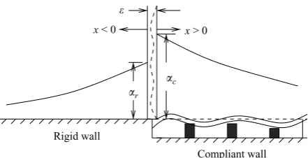
We believe that aspects of our method are generic, but it is presented in the context of a specific problem that is illustrated in figure 1. This depicts a Tollmien–Schlichting (TS) wave incident on a junction at x=1 between a plane channel flow with rigid

and compliant walls. The compliant section of the channel is finite in length, and so there is a second junction at x=2 between the compliant and rigid sections.

This problem was investigated by Davies & Carpenter (1997) using direct numerical simulations.

† Email address for correspondence: [email protected]

Undisturbed velocity profile

Compliant Wall Rigid wall

y = y1 y = h

x = 2 x = ₁

Rigid wall

x = 0

Rigid TS

Rigid TS Compliant TS

Figure 1.Schematic sketch of the problem under study. The figure is taken from figure 2 of Davies & Carpenter (1997).

ε

Rigid wall

Compliant wall

x < 0 x > 0

αr αc

Figure 2.Schematic sketch defining the notation used to analyse the behaviour of the incident and transmitted waves in the neighbourhood of the junction. The broken sinuous curve depicted within the narrow junction zone is intended to depict the wave driver created by the interaction of the incident wave and the junction.

Although the numerical simulations provided a satisfactory solution to the problem, they exhibited certain puzzling features that could not be explained. One of these concerned the spatial development of the perturbation enstrophy and kinetic energy integrals across the two junctions. When the incident wave is below the cutoff frequency of the compliant wall, the only propagating mode is the TS wave (see schematic in figure 2). It is immediately evident from figure 6 of Davies & Carpenter (1997) that in this case there are sharp jumps at the leading-edge junction in the enstrophy and kinetic energy integrals, downwards for the former, upwards for the latter and vice versa at the trailing-edge junction. All simulations with the TS frequency below the cutoff frequency of the compliant wall displayed the same behaviour. Accordingly, the questions remaining unanswered by the numerical simulations are as follows: Why do the jumps occur and why is there a kind of reciprocity relationship between the leading- and trailing-edge junctions?

We now give a brief description of our novel analytical approach to this problem. For the present, to avoid unnecessary complication we shall consider the leading edge of the compliant panel to be the sole junction. Thus we write the perturbation streamfunction in the following form:

ψ(x, y, t) =f(x=x−1, y)e−i¯ωt, (1.1)

We expect the streamfunction to take different forms upstream and downstream of the junction, so we write

f(x, y) =H(−x)fr(x, y) +H(x)fc(x, y), (1.2) where H(x) is the Heaviside step function and suffices r and c denote rigid and compliant walls, respectively. Also plotted in figure 6 of Davies & Carpenter (1997) are the envelopes corresponding to the growing TS wave over an infinitely long rigid wall and the attenuating TS wave over an infinitely long compliant wall. These were obtained by solving the coupled Orr–Sommerfeld compliant-wall eigenproblems for the corresponding homogeneous systems. It is evident that only in the immediate vicinity of the junction do the growth rates of the incident and transmitted waves depart from those corresponding to the (homogeneous) eigenproblems. This suggests that the junction region is very narrow compared with the wavelength of the incident TS wave (see figure 2). If this is so, the functions in (1.2) can be written in the forms

fr(x, y) = Re[aφ¯r(y)ei¯αrx

far field

+f nr(ξ, y) near field

] : x<0, (1.3a)

fc(x, y) = Re[λaφ¯c(y)ei¯αcx

far field

+f nc(ξ, y) near field

] : x>0, (1.3b)

where Re indicates that the real part of the complex quantities is taken, a is the amplitude of the incident TS wave atx= 0 (hereafter taken as unity for the leading-edge junction) and ξ=x/; is assumed to be a measure of the non-dimensional width of the junction region. There is no loss of generality in the forms assumed in (1.3a,b). However, they will only be useful if =O(1). In fact, it will be shown later to be O(Re−1/3) whereReis the Reynolds number. The far-field eigenfunctions

¯

φr and ¯φc and eigenvalues ¯αr and ¯αc, upstream (rigid) and downstream (compliant) of the junction, correspond to suitably normalized eigenmodes of the respective homogeneous systems, andλis an unknown constant representing the amplitude ratio of the downstream to upstream far-field solutions. Assuming that the homogeneous eigenmodes are known, the problem we set out to solve is how to determine the amplitude ratio λwithout detailed knowledge of the near field.

By using half-range Fourier–Laplace transforms (HFLTs) of the governing equation, we show that the junction is equivalent to a virtual local wave driver. This concept is illustrated in figure 2. The problem then reduces to determining the strength of the wave driver. We use the classic theory for inhomogeneous ordinary differential equations, which makes use of the adjoint eigenfunctions, to determine the strength of the virtual driver and the amplitude ratioλ. It is known that near-field effects can be simulated exactly by a virtual wave driver for some simple problems. For example, Carpenter et al. (2002) and Carpenter & Sen (2003) show that this is so for elastic waves propagating along an elastic plate-spring system and incident on a pinned joint with another elastic plate-spring system.

part of the theory. Accordingly, in our theory the adjoint eigensolution plays a sort of reverse role compared with Hill, in that it determines the strength of the vorticity source (or driver) created at the junction by the incident TS wave.

Before presenting our wave driver theory in detail, it may be worthwhile to discuss briefly some other approaches to similar problems that do not work for vortical waves. Many problems involving waves incident on junctions can be solved by using conservation relations. A well-known example is waves along elastic tubes (Lighthill 1978). In this case the reflected and transmitted waves at a junction can be determined in terms of the incident wave by applying continuity of pressure and either conservation of mass or energy; these last two conditions lead to identical results. An example that is similar to the present problem and can be solved by conservation methods concerns waves propagating in a potential flow along a compliant wall with spatially varying stiffness (see Lucey, Sen & Carpenter 2003). At first sight it might appear that conservation of properties such as energy and enstrophy could be used to solve the present problem. It is immediately apparent from figure 6 of Davies & Carpenter (1997), however, that neither quantity is conserved across the junctions. As pointed out above there are jumps in the values of both quantities at the junctions. From the viewpoint of our theory, this is because the near field at the junction, of which the virtual wave driver is an idealization, creates positive, or negative, energy and enstrophy at the junctions.

Another approach that could appear viable is to confine attention to the flow regime downstream of the junction (i.e. over the compliant wall) and to take the upstream incident eigenstate as the initial condition. One might attempt to expand this initial condition in terms of a set of downstream eigenmodes. However, this approach will fail because although the eigenmodes for the two-dimensional Orr– Sommerfeld eigensystem for the rigid-wall channel are bi-orthogonal (Henningson & Schmid 1992), as also are the corresponding ones for the Orr–Sommerfeld compliant-wall eigensystem, neither set of eigenfunctions is complete and it is not possible to describe the compliant-wall eigenfunctions in terms of expansions of the rigid-wall ones or vice versa. In simple terms, the different forms of the wall boundary conditions plainly make it impossible, as can be seen from the forms of the eigenfunctions and their adjoints. Even if such an approach were feasible, it would still be invalid because the near field is completely neglected. That neglecting the near field in this way leads to errors is illustrated by comparing the results of Wiplier & Ehrenstein (2000) and Davies & Carpenter (1997). They adopted an approach whereby the incident TS wave was used as the initial condition at the junction for their direct numerical simulations. The flow fields downstream of the junction produced by their simulations differ significantly from the corresponding simulations obtained using the methods of Davies and Carpenter. This is not surprising because, in effect, the near field upstream of the junction is being ignored. (However, we are not suggesting that this in any way invalidates the study of Wiplier & Ehrenstein.)

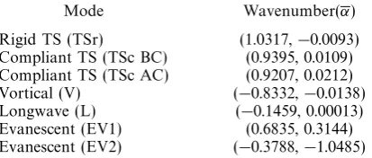
Rigid TS

Compliant TS

Leading edge EV1 Trailing edge EV2

Vortical (V) Long Wave (L)

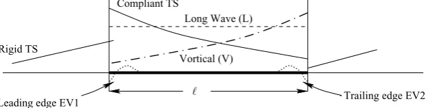
Figure 3. Schematic sketch of the eigenmodes for the case above cutoff frequency of the com-pliant panel. There are three propagating modes present over the comcom-pliant panel. The transmitted TS wave which is damped, a near-neutral almost irrotational damped long-wall wave (L) that propagates downstream from the leading-edge junction and a vortical damped-wall wave (V) that propagates upstream from the trailing-edge junction. There are also evanescent modes (EV1 and EV2) in the vicinity of the junctions.

integrals with respect to x of the jump in the Fourier transform of the potential at y= 0 and its normal derivatives over positive and negative half-infinite ranges. One of the integrals is zero and the boundary conditions at y= 0 and the form assumed for the transformed potential allow relationships to be derived between the remaining integrals. Solving these leads to a solution of the problem. This is typical of the application of the Weiner–Hopf technique. Our method is plainly quite different. Moreover, although we could not entirely rule out the Weiner–Hopf technique as a possible approach, we could see no way of applying it to our problem. A major difference is that the Weiner–Hopf technique leads to the exact solution of a problem, whereas our method seeks to determine the relationship between the far-field solutions without recourse to a detailed knowledge of the near field.

Ours is essentially a receptivity problem. Some specialists in receptivity have made unpublished attempts to solve it using receptivity techniques. For example, Manuilovich (2001), drawing on earlier work (Manuilovich 1992), conceives of the junction as being analogous to a controlled wall motion that creates a TS wave. This is evidently somewhat similar to a wave driver. However, Manuilovich does not actually solve the present problem, originating with Davies & Carpenter (1997). A brief description of his approach is given by Carpenter & Sen (2003). However, in more recent papers (Manuilovich 2003, 2004a, b) the present problem and other similar ones have been investigated.

not been completely suppressed by the time it reaches the trailing-edge junction, both it and the vortical wall mode create separate virtual wave drivers at the junction.

The study in Davies & Carpenter (1997) was mainly motivated by an interest in using a series of short compliant panels to suppress the growth of TS waves, thereby maintaining laminar flow at very high Reynolds numbers. But our problem is plainly related to many biomedical applications; for example, the use of stents to reinforce blood vessels, and pulsatile flows through a stenosis. There are also evident links with the study of collapsible tubes (see for example Heil & Jensen 2003; Grotberg & Jensen 2004), particularly the numerical studies of Luo & Pedley (1995, 1996) and Pedrizzetti (1998). However, these studies are nonlinear, whereas the general problem considered here is linear. In other branches of engineering, similar problems are found in a variety of applications (see for example Nguyen, Pa¨ıdoussis & Misra 1994; Howe 1998; Pa¨ıdoussis 1998).

The remainder of the paper is set out as follows. The formulation of the problem is described in detail in §2. The development of the theory based on modelling the junction as a local virtual wave driver, for the rigid-wall case, is discussed in§3. This problem is extended to the compliant cases in §4. Section 5 discusses the form of the wave driver function. The results are presented and discussed in §6. Finally the conclusions are given in§7.

2. Formulation of the governing equations

2.1. Statement of the fundamental problem

As mentioned earlier, in the present work a channel (plane Poiseuille) flow is considered as the model wave-bearing medium for demonstrating our novel approach to waves propagating across junctions. Also the numerical simulations of Davies & Carpenter (1997) are available for comparison. Furthermore, plane Poiseuille flow is a good choice for the model problem because it is a truly parallel flow with a simple parabolic velocity profile. As shown in figure 1, the rigid-compliant-rigid channel region is formed by having a compliant insert between two rigid sections. The streamwise and wall-normal coordinates are denoted by x and y respectively. The compliant wall properties are applicable in the region fromx=1 tox=2 as shown

in figure 1. The regionsx < 1andx > 2correspond to the rigid-wall channel sections.

The domain from y= 0 to y=h corresponds to the half-width of the channel. The reference length, velocity and time scales used for non-dimensionalization areh, Um and h/Um respectively, where Um is the centreline undisturbed velocity. Henceforth the variables and parameters are dimensionless unless explicitly indicated otherwise. The Reynolds number is given asRe=Umh/ν, where ν is the kinematic viscosity.

Since a two-dimensional parallel flow is being considered, a disturbance streamfunctionψ(x, y, t) can be introduced. The amplitudes of the disturbances are assumed to be sufficiently small for linearized theory to be used throughout. The non-dimensional governing equation, obtained by linearizing the Navier–Stokes equations, is written below in vorticity (∇2_{ψ) form in terms of the disturbance streamfunction:}

∂ ∂t(∇

2_{ψ) + ¯u} ∂ ∂x(∇

2_ψ)−u¯∂ψ ∂x −

1 Re∇

4_{ψ = 0, (2.1)}

where ¯uis the undisturbed laminar velocity profile given as ¯u= 2y−y2_.

and incident on the junction with the compliant section. We consider initially the case when ¯ω is below the cutoff frequency of the compliant wall. Thus the only wave propagating along the compliant section will be the transmitted TS wave. Under these circumstances the streamfunction can take the form of (1.1) and substituting this into (2.1) gives the operative differential equation for the problem, namely

−i¯ω(∇2f) + ¯u ∂ ∂x(∇

2_f)−¯u∂f

∂x − 1 Re∇

4_{f = 0. (2.2)}

Following Davies & Carpenter (1997) we restrict attention to normal disturbance velocity components v that are symmetrical (implying antisymmetrical streamwise disturbance componentsuand symmetrical disturbance streamfunction and vorticity), because disturbances of this type determine the stability in the case of rigid walls (Drazin & Reid 1981). Thus for the rigid- and compliant-wall sections alike of the channel, the boundary conditions at the centreline are

fy(x,1) =fyyy(x,1) = 0, (2.3a, b) where suffices y andx denote partial differentiation with respect to these variables.

On the rigid wall the usual no-penetration and no-slip conditions hold, i.e.

fx(x,0) =fy(x,0) = 0. (2.4a, b) On the compliant wall these, when linearized about y= 0, take the form (see for example Carpenter & Garrad 1985)

fx(x,0) = i¯ωη,ˆ fy(x,0) + ¯u(0) ˆη= 0, (2.5a, b) where η= ˆηexp(i¯ωt) is the wall displacement. Equations (2.5a) and (2.5b) can be combined in a single boundary condition of the form

fy(x,0)− i¯u(0)

¯

ω fx(x,0) = 0. (2.6)

The remaining boundary condition at the wall is derived from the equation of motion for the compliant wall. Following Davies & Carpenter (1997) we use the plate-spring compliant-wall model of Carpenter & Garrad (1985). Accordingly the wall displacement η is only in the y direction and is governed by the following equation of motion:

m∂ 2_η

∂t2 +d ∂η ∂t +B

∂4η

∂x4 +Kη = −pw, (2.7)

where pw is the unsteady hydrodynamic pressure acting on the wall and the non-dimensional wall parameters are defined as follows in terms of non-dimensional quantities denoted by an asterisk:

m= m

∗

ρh, d∗ ρUm ≡

1 Re

d∗ρh

ν ≡

d Re, B∗

ρh3_U2 m

≡ 1

Re2 B∗ ρhν2 ≡

B Re2,

K∗h ρU2 m

= 1

Re2 K∗h3

ρν2 = K

Re2, (2.8)

wherem∗,d∗, B∗ andK∗ are respectively the mass per unit length, damping, flexural rigidity and spring stiffness of the plate-spring system.

If the plate is pinned at each junction,

η= ∂

2_η

whereas for clamped end conditions

η= ∂η

∂x = 0 at x=1, 2. (2.10a, b) Pinned joints were assumed in Davies & Carpenter (1997), but there is no difficulty in carrying out numerical simulations for clamped end conditions, and some results for such end conditions will be presented below.

Two things are required to convert (2.7) into a boundary condition for the streamfunction f. First, we need to replace η as the variable with ˆη, and then substitute for ˆη using (2.5a). Second, we need a way of determining the wall pressure pw= ˆpwexp(−i¯ωt). In Davies & Carpenter (1997) we used the linearized y-momentum equation to determine pw as an integral with respect to y across the channel. This is very convenient for our particular form of numerical simulation. In the present context, however, it has the disadvantage of leading to a non-standard form for the boundary condition that makes it difficult to apply the classic theory for inhomogeneous systems of ordinary differential equations (see for example Ince 1926). So, as an alternative, we follow Carpenter & Garrad (1985) and use the linearized x-momentum equation that takes the form

ˆ pwx+

1

Re(fyxx(x,0) +fyyy(x,0)) = 0. (2.11) Note that the inertial terms are omitted in (2.11) because they sum to zero aty= 0 on account of the no-slip condition, as given in (2.5b).

In§2.2 below, the final forms of the boundary conditions are formulated after the HFLTs have been taken.

The two-dimensional TS wave incident on the leading-edge junction at x = 1

undergoes a jump in amplitude, as discussed above. Another apparently near-reciprocal jump in amplitude occurs at the trailing-edge junction at x=2 (see

figure 1 and Davies & Carpenter 1997). One needs to understand the conditions at the junctions, x=1 and x=2, to understand why these jumps occur and to

determine the transmitted wave and, in some applications, the reflected wave at each junction. Figure 2 also depicts schematically typical growth curves for the disturbance waves either side of the junctions. This behaviour will be explained in later sections.

2.2. The Fourier–Laplace transformed system of equations

Half-range Fourier–Laplace transforms (HFLTs) in terms of wavenumberα are now defined for f(x, y) =fr(x, y)H(−x) +fc(x, y)H(x), again in two halves, for either side of the junction. (For simplicity we will work with a shifted streamwise variable x=x−1 that has its origin at the junction.)

Fr(y, α) = 0

−∞

fr(x, y)e−iαx

dx, (2.12a)

Fc(y, α) = +∞

0

fc(x, y)e−iαx

dx. (2.12b)

The form of the solutions must be such that away from the immediate vicinity of the junction they reduce to the far-field TS waves. Thus we expect them to take the forms given in (1.3a,b). The inverse transforms are also defined separately for −∞< x60 and 06x<∞ and can be evaluated as follows:

fr(x, y) = 1 2π

Cr

Fr(y, α)eiαx

fc(x, y) = 1 2π

Cc

Fc(y, α)eiαx

dα, 06x<∞, (2.13b)

where Cr and Cc are suitable contours enclosing the poles. The above method of representation is most convenient for showing that the junction can be modelled as a local virtual wave driver. This is demonstrated below.

First, it is important to note how derivatives with respect to x are dealt with for HFLTs. Thus, using integration by parts, the HFLT of the first derivative of the stream functions,fr,c(x, y), upstream and downstream of the junction are given by

0

−∞

∂fr ∂xe

−iαx_d

x=fr(0, y) + iαFr(y;α), (2.14a)

_∞

0 ∂fc ∂xe

−iαx

dx=−fc(0, y) + iαFc(y;α), (2.14b)

using repeated integration by parts, the HFLTs of the corresponding higher derivatives are given by

0

−∞

∂nfr ∂xne

−iαx dx =

n

k=1

(iα)k−1f_r(n−k)(0, y) + (iα)nFr(y;α), (2.15a)

_∞

0 ∂n_f

c ∂xne

−iαx

dx =− n

k=1

(iα)k−1f_c(n−k)(0, y) + (iα)nFc(y;α). (2.15b)

Other variables are dealt with in a similar fashion.

Taking the HFLT of the operative differential equation (2.2), and making use of the results given in (2.14a,b) and (2.15a,b), we obtain the following pair of equations:

L(α)Fr,c=±ω¯ ⎧ ⎪ ⎪ ⎪ ⎨ ⎪ ⎪ ⎪ ⎩

αfr,c+ i

∂fr,c ∂x

O(1/)

⎫ ⎪ ⎪ ⎪ ⎬ ⎪ ⎪ ⎪ ⎭

x=0

±¯u ⎧ ⎪ ⎪ ⎪ ⎨ ⎪ ⎪ ⎪ ⎩

−α2fr,c+ iα

∂fr,c ∂x

O(1/)

+

∂2_f

r,c ∂x2

O(1/2₎

⎫ ⎪ ⎪ ⎪ ⎬ ⎪ ⎪ ⎪ ⎭

x=0

∓¯u{fr,c}x=0

∓ 2 Re ⎧ ⎪ ⎪ ⎪ ⎨ ⎪ ⎪ ⎪ ⎩

iαfr,c +

∂f_r,c ∂x

O(1/)

⎫ ⎪ ⎪ ⎪ ⎬ ⎪ ⎪ ⎪ ⎭

x=0

∓ 1 Re ⎧ ⎪ ⎪ ⎪ ⎨ ⎪ ⎪ ⎪ ⎩

−iα3fr,c−α2

∂fr,c ∂x

O(1/)

+iα

∂2_f r,c ∂x2

O(1/2₎

+

∂3_f

r,c ∂x3

O(1/)3

⎫ ⎪ ⎪ ⎪ ⎬ ⎪ ⎪ ⎪ ⎭

x=0

whereL(α) is the linear Orr–Sommerfeld operator, namely

L(α)F = i(αu¯−ω¯)(F−α2F)−iα¯uF − 1 Re(F

_−2α2_F+α4_{F). (2.17)}

In the above, (2.16a) and suffix r correspond to x<0 whereas (2.16b) and suffix c correspond tox>0. Also, when ±and∓are used the upper symbol corresponds to (2.16a) and the lower to (2.16b). Also, assuming for now that the form proposed in (1.3a,b) is valid, the order of magnitude of each derivative off with respect tox, at x= 0, is indicated below the respective terms. These follow from the forms assumed in (1.3a,b). Superscript prime denotes derivatives with respect toy.

As it is a solution of the Navier–Stokes equations, f and all its derivatives are continuous everywhere within the fluid domain including at the junction. This does not, however, strictly apply at the point (x= 0, y= 0) where, depending on the type of joint assumed between the rigid and compliant walls, any of the second and higher derivatives of f could be discontinuous. For example, recalling from (2.5a) that η ∝ fx(x,0), for pinned joints (see (2.9a,b)), fx(x,0) =fxxx(x,0) = 0 as x →0+ _{and so are continuous along the wall at the junction, but f}

xx(x,0) is not. This minor difficulty arises because in the immediate vicinity of the pinned joint the natural coordinate system is polar centred at the joint, rather than Cartesian. It is straightforward, using a polar coordinate system, to demonstrate that all derivatives of the streamfunction are continuous functions of the azimuthal coordinate as the radial coordinate tends to zero and that the streamfunction is well behaved. Accordingly, for the general case we shall write (2.16a,b) in the form

L(α, ω)Fr =Rr, (2.18a)

L(α, ω)Fc=−Rr−(1−H(y−0+)) ⎛ ⎜ ⎝u Δ¯1

O(−2₎ − 1

Re(iαΔ1 O(−2₎

+Δ2) O(−3₎

⎞ ⎟

⎠, (2.18b)

whereRr denotes the right-hand side of (2.16a),Δ1=fc,xx(0,0) andΔ2=fc,xxx(0,0); Δ1= 0 for clamped joints but is non-zero for pinned ones, whereas for Δ2 it is the

other way round. This is somewhat similar to flow past a corner. It will be seen later on that the right-hand sides of (2.18a,b) are used only as weighted definite integrals in the domain y= 0 to y= 1; therefore, towards this end owing to the presence of the term (1−H(y−0+)), the last term on the right-hand side of (2.18b) makes little contribution. Hence the term involving (1−H(y−0+)) is neglected from hereon and not brought up in future discussions.

It is also necessary to determine the boundary conditions for the transformed streamfunction. For the centreline the end conditions atx= 0 make no contribution and the boundary conditions (2.3a,b) become

Fr,c (1;α) =Fr,c(1;α) = 0. (2.19a,b) Likewise forx<0, the wall boundary conditions (2.4a,b) become

Fr(0;α) =Fr(0;α) = 0. (2.20a,b) Forx>0, (2.6) becomes

Fc(0;α) + i αu¯(0)

¯

Taking the HFLT of the expression (2.11) for wall pressure, after minor rearrangement we obtain

Pc(0;α) =− i αRe[F

c (0;α)−α 2_F

c(0;α)], (2.22) wherePc is the HFLT of ˆpw.

After substituting (2.22), the HFLT of (2.7) for the wall motion becomes

iα

2

¯ ω(α

4

B+K−i d¯ω−mω¯2)Fc(0;α) + 1 Re[F

c (0;α)−α 2

Fc(0;α)] = 0. (2.23)

A fully equivalent alternative formulation of (2.23) could be derived using the concept of admittance introduced by Landahl (1962) (see Carpenter & Garrad 1985; Sen & Arora 1988). This approach was used in the earlier versions of our theory (see Carpenter et al. 2002; Hegde 2002; Sen, Hegde & Carpenter 2002, 2003; Carpenter & Sen 2003). The present approach has been adopted to show more clearly how the boundary conditions are treated in the analysis.

To proceed further, we take an important step forward to replace the near-field derived termRr on the right-hand side of (2.18a,b) by a discrete structure inxlocated at x= 0 having an amplitude distribution in y as F(y). This step is analogous to replacing the thin viscous shock wave in compressible flow by an inviscid discontinuity. The function F(y) is called the wave driver function, or driver function. Thus we can restate the governing system of linear ordinary differential equations (2.16a,b) with boundary conditions (2.19a,b), (2.20a,b), (2.21) and (2.23) in the following more succinct forms:

L(α, ω)Fr =CF(y), (2.24a)

L(α, ω)Fc=−CF(y), (2.24b)

whereF(y) is anO(1) function, the form of which remains to be determined, andC is a constant, called later the driver strength, the order of magnitude and values of which remain to be determined. It will be shown later that C∼O(Re2/3_{). Also note}

the opposite signs for F(y) respectively on the right-hand sides of (2.24a, b). This is because the wave driver is not a discrete ‘source’ in the conventional sense of the term. Rather, it is a novel discrete structure which is a ‘half source cum half sink’; a ‘source’ for the outgoing wave and a ‘sink’ for the incoming wave. Other properties of the wave driver will be brought out later on. At the moment we note that the wave driver represents a strongly vortical structure, since it is a discretization of the (highest order) termu(∂2_f)/(∂x2_)|x

= 0, in (2.16a,b).

The boundary conditions, for the rigid side and for the compliant side, may be gleaned from (2.19) to (2.23), which are respectively given as follows:

Fr(1) =Fr(1)= 0, Fr(0), Fr(0) = 0. (2.25a,b,c,d)

Fc(1) =Fc(1)= 0; (2.26a,b)

The key questions now are: How can a suitable driver functionFbe determined? And, givenFhow can the constantC and the amplitude of the downstream far-field wave be determined? Before these questions are addressed in §4, we first apply our basic method immediately below in§3 to the much simpler case of finding the far-field solution for the case of a known driver function.

3. Tollmien–Schlichting waves generated by a known driver

In order to provide a relatively simple illustration of our basic approach we shall first consider the generation of TS waves in a rigid-wall plane Poiseuille flow. Let us suppose that the driver is located at x= 0 and that it varies harmonically in time with frequency ¯ω just as in the case of the problem described in §2. In the far field downstream of the driver, providing ¯ω and the Reynolds number Re lie within the region of instability, we would expect to find a spatially propagating TS wave. We shall show below that the amplitude of this downstream-propagating wave can be determined in terms of the known driver function without determining all the details of the near field. In many respects this problem is similar to the one involving the generation of a TS wave in a boundary layer by an idealized driver representing a vibrating ribbon. This problem was first investigated by Gaster (1965) and revisited by Ashpis & Reshotko (1990). Here the problem is simpler because the flow is truly parallel and the continuous spectrum is absent.

The governing equation in the Fourier–Laplace domain is similar to (2.24), namely L(α,ω¯)F =−CF(y), (3.1a) which can be written in the form

[L1(α) + ¯ωL2(α)]F =−CF(y), (3.1b)

where

L2(α)F =−i(F−α2F), L1(α)F = [L(α,ω¯)−ωL¯ 2(α)]F, (3.1c,d)

where, in (3.1a, b), the minus sign appears on the right-hand side because we are interested in the domain x >0 and propagation downstream. Let us suppose that CF(y) represents a known function that is specified in advance. The far-field solution forF is expected to take the form

aφ¯(¯α,ω¯) α−α¯ ,

where ¯α is the appropriate spatial rigid-wall eigenvalue and ¯φ the corresponding normalized eigenfunction. The object of the exercise is to determine a value of the amplitudeaof the far-field TS wave in the physical domain in terms ofCF(y). Here a is proportional toa. Further, since we will be confining ourselves to the rigid wall in this section, we will omit using the subscript ‘r’.

3.1. The theory

way would be if we could expand CF(y) as a suitable eigenfunction expansion. In fact we were able to do just this, and also so, in a very convenient way. At this stage we introduce the concept of generalized temporal eigenstates. It will become clear why this is advantageous. For every complex value of α there exists an infinite number of eigenstates characterized by complex values of ω. Let us denote these by

˜

φk(α,ω˜k), k= 1,2, . . . ,∞; L(α,ω˜k) ˜φk= 0, (3.2a,b) such that ˜φk → φ¯k and ˜ωk → ω¯k (k= 1,2, . . . ,∞) as α → α¯. Note that ¯ω1( = ¯ω),

which is the driver frequency, is actually real and is not the conventional temporal eigenvalue of hydrodynamic stability theory, although the absolute values will be close. We remember further that all the ˜φk,φ¯k are normalized eigenfunctions. Henceforth we shall use the following convention regarding notation: ¯q will denote quantity, q, corresponding to the imposed or driver frequency ¯ω and far-field wavenumber ¯α, whereas ˜qwill denote quantities corresponding to the generalized temporal eigenstates corresponding to α= ¯α.

It is known for plane Poiseuille flow that any arbitrary transverse distribution of the perturbation streamfunction can be expressed as an infinite sum of the discrete temporal eigenfunctions,φk(k= 1,2,3, . . .),or, equivalently, of the setφk−α2φk. No equivalent theorem appears to have been established for the spatial eigenfunctions. It is widely assumed (see for example Schmid & Henningson 2001) that provided the appropriate set is chosen depending on whether one is computing upstream or downstream response, the perturbation streamfunction in this case also can be represented as an infinite sum of spatial eigenfunctions. It has been mentioned in the previous section that our driver function is not completely arbitrary, and is strongly vortical in content. There will be some discussions in the next section as to how the actual form of the driver function may be educed. It can however be seen from (2.16a,b) that the largest contribution to the driver should come from the term

CF(y)∼u¯ ∂

2_f

∂x2

x=0

. (3.3)

Accordingly, it seems perfectly reasonable to represent the driver function in the present case in terms of the temporal eigenfunctions ˜φk. But before we proceed further we must hasten to answer the question ‘why do we use a temporal eigenfunction expansion, in terms of ˜ωk, rather than a spatial eigenfunction expansion?’ The answer is direct and straightforward. There is an algebraic nonlinearity in α in the basic Orr–Sommerfeld equation (2.17) which renders a simple decomposition analogous to (3.1b) unfeasible. The advantage of using a decomposition like (3.1b) will become obvious in the next few steps because the solutions can be virtually read off. Hence we expand the driver function in the following form, at any α, not necessarily equal to ¯α:

CF(y) =

∞

k=1

˜

bk˜gk, (3.4)

where

˜

gk=−i( ˜φk−α 2_φ˜

k). (3.5)

˜

φk(α,ω˜k), so that

1

0

˜

θk˜gjdy =δj k

1

0

˜

θkg˜kdy, (3.6)

whereδj k= 1 whenj=k and is zero otherwise. Thus the coefficients in (3.3) are given by

˜ bk=

1

0 CF(y)˜θkdy 1

0 ˜θk˜gkdy

. (3.7)

Next we will develop the solution asα→α¯ and ˜ωk →ω¯k. Particularly we will call ¯

ω1= ¯ω, where ¯ω is the actual physical driver frequency. Further we note from (2.17)

that

Lω(α,ω˜k) ˜φk =L2(α) ˜φk= ˜gk, L2(¯α) ¯φk = ¯gk. (3.8) We proceed further as follows:

L(α,ω¯)F = [L1(α) + ¯ωL2(α)]F =−

∞

k=0

˜

bk˜gk. (3.9)

The above step is a precursor to the introduction of the generalized eigenfunctions ˜

φk (k= 1,2,3, . . .). We now expandF in terms of ˜φk (see (3.2a, b)) as follows:

F =

∞

k=1

˜

akφ˜k(α,ω˜k) =

∞

k=1

˜ a_k ˜ ωk−ω¯1

˜

φk(α,ω˜k), (3.10a, b)

where allak areO(1). Note that asα→α¯ then ˜ω1 →ω¯1 = ¯ω and only the first term

in the series is singular (as will be shown below, it has to take this form in order to recover the correct form of the far-field downstream wave after taking the inverse Fourier–Laplace transform); it is only for convenience that the coefficients of the remaining terms are written with denominators in the forms of differences in complex frequency. We now substitute forF from (3.10) into (3.9). Thereafter, for each value ofk we have

˜

akL(α,ω¯) ˜φk= ˜ak[L1(α) + ˜ωkL2(α)] ˜φk

−(˜ωk−ω¯)˜akg˜k= ˜bkg˜k, (3.11a) where, by definition, the terms in underbrace, viz.

[L1(α) + ˜ωkL2(α)] ˜φk =L(α,ω˜k) ˜φk = 0. (3.11b) We now get a formal solution for ˜ak, from (3.11a, b), as follows:

˜ ak =

˜ bk (˜ωk−ω¯)

, (3.12a)

and remembering (3.10) we have ˜

ak = ˜bk. (3.12b)

It therefore appears that the solution to (3.9) can virtually be read off, in terms of the generalized eigenstates ofL(α,ω˜k) ˜φk= 0. Now we go to an important limit when α→α¯and ˜ω1→ω¯1(= ¯ω). This leads to the singular term in (3.1) fork= 1. Moreover,

The singular solution Fs, corresponding to the far-field downstream TS wave, is given by settingk= 1 in (3.10), and going to the limitα→α¯, which also gives ˜φ1→φ¯.

Hence we obtain the following:

Fs = ¯φ I2

(˜ω1−ω¯)I1

= ¯φ I2 (α−α¯)cgI1

, (3.13a)

where

I1 =

1

0

¯

θg¯dy, I2=

1

0

CF¯θdy, cg = dω

dα, (3.13b, c, d) wherecg is the complex group velocity.

In order to determine the far-field solution in the physical plane we need to carry out an inverse Fourier–Laplace transformation of (3.13a). Calling the Fourier–Laplace inverseF−, we have

F−[Fs] =f(x, y), f(x, y)e−i¯ωt =aφ¯ei(¯αx−ωt¯), (3.14a, b) where a is the amplitude of the normalized far-field eigenfunction ¯φ. Also, from (3.13–3.14) we have the inverse transform as

aφ¯ei(¯αx−ωt¯)= φ¯e

−i¯ωt

2πcg I2 I1

Cr eiαx

α−α¯dα, (3.15a)

Cr eiαx

α−α¯dα= 2iπe

i¯αx

, (3.15b)

whereCr is an appropriate contour of integration. Therefore, we have

aφ¯ei(¯αx−ωt¯) = i cg

I2 I1

¯ φei

¯ αx−ωt¯

. (3.15c)

Hence the all important amplitude a of the normalized far-field eigenfunction ¯φ is given as

a= iI cg

, I = I2 I1

. (3.15d, e)

Thus the amplitude of the downstream TS wave is now given in terms of the driver function by (3.1a, b, c, d). In the end we see that the procedure comes out to be astonishingly simple. Given a driver function F(y) (of strength C) all we need to determine the amplitude aof the far-field solution are the integralsI1 andI2 and the

group velocity cg.

3.2. Application of theory to a known driver

To illustrate the application of the theoretical approach outlined above let us consider a driver that takes the form of an oscillating velocity imposed at the wall taking the form

vw= ˆvwδ(x)eiωt. (3.16a) A driver of this form was used by Gaster (1965). For numerical simulations it is necessary to approximate the delta function and write the driver as

ˆ vw √πe

−(x/)2

Using the methods described in Davies & Carpenter (1997) we carried out a numerical simulation using this driver with Re= 12 000, ¯ω= 0.24, = 0.125 and ˆ

vw= √

π. As expected, a growing TS wave was generated downstream with a complex wavenumberα= (1.0317,−0.0093) in good agreement with the values we determined from hydrodynamic stability theory. This far-field solution,

v(x, y, t) =−∂ψ

∂x =−iaαφ¯r(y) ˆ v

ei(αx−ωt)_{, (3.17)}

can be extrapolated backwards to the origin in order to determine the corresponding amplitude of the normal velocity on the centreline, namely−iaα, provided we adopt a normalization whereby ¯φr(1) = (1.0,0.0). (Again we introduce the generic subscript ‘r’ for the rigid wall). Hence we obtain the value of the amplitude of the streamfunction asa= (−0.19,−0.06) = 0.20ei1.1π_.

We shall now calculate this quantity using our theoretical result, (3.15d, e), with the driver function approximated in the form given in (3.3). It will be shown in §5 that this approximate form relies for its validity on the width of the driver region being sufficiently narrow to drop all the terms but one on the right-hand side of (2.16). Note, however, that the width of the present driver, namely = 0.125, is an order of magnitude greater than that of the virtual wave driver in§5. Thus, although the neglected terms on the right-hand side of (2.16) will remain secondary, their contribution cannot be expected to be completely negligible.

A further subtlety concerns the approximation of the delta function. If we were actually using a delta function then d ˆvw/dx=δ(x). Thus we need to find a suitable approximation to δ(x) that corresponds to the numerical simulation. This can be given from the form in (3.16), from which it follows that the driver wall-normal perturbation velocity is given by

v(x, y) = vˆ(y) √πe

−(x/)2

(vˆ(y)δ(x)). (3.18)

It may be seen in (2.16) earlier, and also later on in discussions following (5.4), that when a stationary narrow vortical structure exists in the fluid side, the largest order term is as given by (3.3). The vibrating ribbon-like disturbance, given by (3.18), is also expected to create a vortical structure above itself in the fluid side. The existence of such a vortical structure is confirmed by the numerical simulations. Remembering in (3.3) that the quantityf is the streamfunction, we therefore have the driver function approximated as follows:

¯ u∂

2_f

∂x2 ¯u(y) ˆv(y)

1 √π

∂ ∂x(e

−(x/)2 )

δ(x)

. (3.19)

Thus the generalized function δ(x) is approximated and replaced by the regular function

1 √π

∂ ∂x

e−(x/)2

=−√2

π2 _x

e−(x/)2

. (3.20)

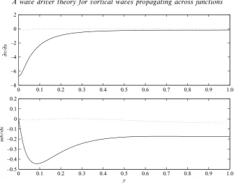
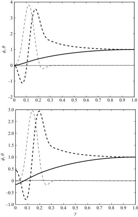
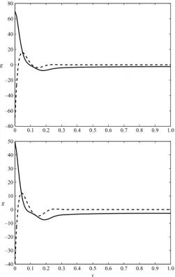
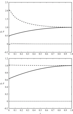
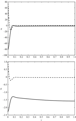
The variation in y of ∂v/∂xˆ and ¯u∂v/∂xˆ are obtained from the numerical simulations, and are plotted in figure 5; the corresponding eigenfunction ¯φr, adjoint eigenfunction ¯θrand the vorticity function ¯gr are plotted in figures 6 and 7 respectively. The value of the integral in the numerator of (3.7), i.e (3.13c), is determined numerically using the data given in figure 5 and a complex value of (0.308,0.153) obtained, when the approximation (3.18), for δ(x), is kept in. The integral in the denominator of (3.7), i.e (3.13d), is similarly found to have a complex value of (−1.847,6.285), and the complex group velocity is obtained as cg= (0.325,−0.042). Thus (3.15a) gives a(−0.17,−0.045)0.18ei1.07π_{. Given that the driver is relatively}

wide, the theoretical value of a seems to be in reasonable agreement with the value ofa= 0.20ei1.1π _{given above, which was determined from the numerical simulation.}

4. The wave driver theory

4.1. Characteristics of the wave driver

We begin this section by listing out some of the important characteristics of the wave driver. Some of these have already come in the previous discussions. Some more characteristics will come forth in the subsequent discussions. The main characteristics are the following:

1. The wave driver is an idealized discrete structure, formed in the fluid side, at the junction of two different wave-bearing media, like rigid-compliant or compliant-rigid walls.

2. The wave driver is an idealized discrete structure that purports to capture some important features of the narrow viscous interface that is known to form when a disturbance wave crosses a junction. Thus the wave driver is associated with an incoming wave and an outgoing wave, respectively belonging to the different wave-bearing media on either side of the junction, like rigid-compliant or compliant-rigid. 3. The wave driver is strongly vortical in content and is neither associated with nor causes any wall displacement at its point of location at the junction.

4. The wave driver is a discrete structure hitherto not used in any past work. It is actually a ‘half source cum half sink’. It behaves like a sink for the incoming wave, and like a source for the outgoing wave. The ‘source’ part of the wave driver is similar to the classically known, and used, sources, for example the vibrating ribbon, from which near-neutral waves (both amplified or damped) can tune out and reach the far field. The ‘sink’ part is something new and its precise nature will come out in the course of subsequent discussions.

5. The wave driver cannot support, nor is by itself responsible for, any wave reflection. This is because it is essentially a structure in the fluid side, and there is no natural barrier in the fluid side that can support a wave reflection.

6. Both the incoming wave and the outgoing wave at a wave driver must be strongly vortical; it is then that the vortical structure, viz. the wave driver, actually comes to exist.

7. The wave driver, being strongly vortical in content, cannot be formed by an incoming near-inviscid wave, i.e. by an incoming wave that has very small vorticity. Likewise, a near-inviscid, or nearly non-vortical, wave cannot tune out of an already existing wave driver. Inviscid waves come to exist because of wall displacement or can tune out from a wall-displacement source (cf. Lucey et al. 2003).

waves tuning out of this existing wave driver. However, such specific possible cases need to be considered individually and carefully.

9. Across a wave driver at a junction the direction of energy propagation must be consistent. This point will be discussed in greater detail later on in this section.

10. Conservation of energy between the incoming and outgoing waves across the wave driver is not addressed to in the present wave driver theory. It is well known from the simulations in Davies & Carpenter (1997) that the near field at a junction comprises complex production and dissipation processes. However, detailed study of the near field is not part of the present work.

4.2. The incoming rigid-side TS wave at the leading-edge junction

Next we consider the incoming rigid-side TS wave that approaches the leading-edge junction. The analysis is very similar to what has been outlined earlier in§3.1, except that there is a sign reversal throughout because the relevant base equation is (2.24a). Using the generic subscript ‘r’ for the rigid side, we have the amplitudear of the rigid side, in relation to the driver functionCF(y), given from (3.15d,e) as follows:

ar =− iCIr

cgr

, Ir = I2r I1r

, (4.1a,b)

I1r = 1

0

¯

θrg¯rdy, I2r =

1

0

F¯_{θrdy, cgr =} dω

dα, (4.1c,d,e) wherecgr is the group velocity of the rigid-side TS wave. Note the slight difference in forms between (3.13c) and (4.1d) and between (3.15d) and (4.1a),C having been kept outside the integrals in (4.1a) and (4.1d). If we specify the rigid-side wave amplitude ar to be the reference amplitude, we may put ar= 1. Then, we are able to estimate the driver strengthC, from (4.1a–e), as follows:

C=icgr Ir

. (4.2)

A rough estimate of the order of C may be made using the Tollmien scale for the viscous critical layer which gives the width of the viscous critical layer in the Orr– Sommerfeld solution,c, asc∼O(Re−1/3). This gives the order of ¯φr as ¯φr∼O(Re

2/3_).

Further, ¯gr is dominated by ¯φr, and also it is well known that ¯θr∼φ¯r. Hence it is easy to estimate from (4.1) and (4.2) that the order of the driver strengthC is given as

C∼OR2/3. (4.3)

The adjoint Orr–Sommerfeld equation for the adjoint eigenfunction θ together with its boundary conditions over a compliant wall are given in the Appendix.

4.3. Wave driver theory for the compliant side

We now focus attention on the compliant side. The basic equation in the Fourier– Laplace domain for the compliant side is given from (2.24a,b) as follows:

of the compliant-wall boundary conditions, which need to be considered very carefully. We must also note that Fc can have only one unique set of boundary conditions. Thus, if we think of an eigenfunction expansion forFc, like ˜φck (k= 1,2,3, . . .), then, all the ˜φckneed to satisfy the same set of boundary conditions. For the rigid-wall case this was not a problem because all the ˜φrk satisfy the same homogeneous boundary conditions at the wall, viz. ˜φrk(0),φ˜rk (0) = 0. For the compliant case the boundary conditions are given by (2.26a–d), reproduced here below:

F_c(1) =Fc(1)= 0, (2.26a,b& 4.5a,b) F_c(0) +a(α, ω)Fc(0) = 0, Fc(0) +b(α, ω)Fc(0) = 0. (2.26c,d & 4.5c,d) It was mentioned in the discussions following (2.26c,d) that ‘the specific choices of α and ω, in a(α, ω) and b(α, ω), will depend on specific situations’. It is time now to address this issue. As α → ¯α, then α and ω, in a(α, ω) and b(α, ω), should also approach ¯α and ¯ω. There are two routes by which this may happen, respectively called ‘Route A’ and ‘Route B’. These are discussed next.

Route A: Suppose that (α, ˜ωc1) is a compliant (and physically possible) eigenvalue

pair, with the corresponding eigenfunction ˜φc1. This is an eigensolution neighbouring

the far-field eigenvalue pair (¯α,ω¯). Also, suppose, as previously described in §3 earlier, we have a system of eigenfunctions ˜φck(k= 1,2,3, . . .) satisfying the following equation and boundary conditions:

L(α,ω˜ck)˜φck= 0, k= 1,2,3, . . . , (4.6) ˜

φck (1) = ˜φck(1)= 0, (4.7a,b)

˜

φck (0) +a(α,ω˜c1)˜φck(0) = 0, φ˜ck(0) +b(α,ω˜c1)˜φck(0) = 0. (4.7c,d) The key feature in the above wall boundary conditions (4.7c,d) is that all the wall boundary conditions, for all the ˜φck (k >1), correspond to a,b being frozen to a(α,ω˜c1) andb(α,ω˜c1). This way, only ˜φc1 is a physically possible eigenfunction. The

remaining eigenfunctions ˜φck (k >1) are non-physical eigenfunctions that have been introduced to be able to solve (4.4a,b), for Fc, in Fourier–Laplace space. We now write an eigenfunction expansion forFc, on the lines of (3.10a,b), as follows:

F =

∞

k=1

˜

ackφ˜ck(α,ω˜ck) =

∞

k=1

˜ a_ck ˜

ωck−ω¯c1

˜

φck(α,ω˜ck). (4.8a,b)

Note that the expansion retrieves the singular and regular parts of Fc= [Fc]s+ [Fc]r, viz. [Fc]s,[Fc]r respectively, as α → α¯c, when also ˜ωc1 → ω¯, ˜φck → φ¯ck and ˜φc1 →

¯

φc1( = ¯φc). The other point to note is that, in view of (4.7c,d) and (4.7a,b), both [Fc]s and [Fc]r satisfy the same wall boundary conditions and same outer boundary conditions. The solution is therefore legitimate and approaches the limitα→α¯c in a natural way.

The rest of the analysis is similar to that in §3.1, and in §4.1 above, for the rigid case, except that the generic subscript ‘c’ is used throughout. Also the equivalents of (3.4) for the expansion of F(y) and the Fourier–Laplace inversion integral (3.15b) are given respectively as

F(y) =

∞

k=1

˜

bckg˜ck, (4.9)

Cc eiαx α−α¯c

where Cc is an appropriate integration contour for the Fourier–Laplace inversion integral in (4.10). The final answer for the amplitude ac for the far-field compliant wave is given similarly as in (4.1a,b) and (4.1c–e) for the rigid case, that is

ac= iCIc

cgc

, Ic= I2c I1c

, (4.11a,b)

I1c= 1

0

¯

θc¯gcdy, I2c=

1

0

F¯_{θcdy, cgc=} dω

dα, (4.11c,d,e) where cgc is the regular group velocity for the far-field compliant wave. For the present ‘Route A’, where the pair (α,ω˜c1) is a neighbouring physical eigenvalue to the

far-field compliant eigenvalue pair (¯αc,ω¯), it is obvious that the regular group velocity cgcfor the far-field compliant wave needs to be used in (4.11a). Also the sign reversal in (4.11a), as compared to (4.1a) for the rigid case, is because it is being assumed that we are at the leading-edge junction where the rigid-side wave is the incoming wave and the compliant-side wave is the outgoing wave.

We now have a method of determining the amplitude ratioλc of the compliant-side to rigid-side amplitude. This is also called the ‘jump in amplitude’. Remembering that we determined the driver strength C in (4.2) above, by keeping the rigid-side amplitudear asar= 1, we have the amplitude ratioλc given as follows:

λc=

ac ar

= iCIc cgc

=−cgr cgc

Ic Ir

. (4.12a,b,c)

In closing we mention that we have considered the above example with reference to the leading-edge junction. However, at this point we are not saying that Route A is appropriate, or not, to the leading-edge junction. This point will come up in a natural way after Route B is discussed.

Route B: We begin the description of Route B by introducing the generic circumflex accent, i.e. ‘(ˆ)’, for all the associated quantities in this route. Analogous to the case in Route A we have a system of eigenfunctions ˆφck (k= 1,2,3, . . .) satisfying the following equation and boundary conditions:

L(α,ωˆck) ˆφck= 0, k= 1,2,3, . . . , (4.13) ˆ

φck(1) = ˆφck(1)= 0, (4.14a,b) ˆ

φ_ck(0) +a(¯α,ω¯) ˆφck(0) = 0, φˆck(0) +b(¯α,ω¯) ˆφck(0) = 0. (4.14c,d) The key feature in the Route B wall boundary conditions (4.14c,d) is that all the wall boundary conditions, for all the ˆφck (k >1), correspond to a,b being frozen to a(¯α,ω¯) andb(¯α,ω¯). This way, none of the eigenfunctions ˆφck (k >1) is a physically possible eigenfunction. Also we remember that ˆφc1→φ¯c, and ˆωc1 →ω¯ when α→¯αc. Moreover, we emphasize that ˆφc1 is also not a physically possible eigenfunction when α= ¯αc. Again, the fact that all the ˆφck are not physical eigenfunctions is not of much consequence because these non-physical eigenfunctions have been introduced to be able to solve (4.4a,b), forFc, in Fourier–Laplace space. The rest of the mathematics is very similar to Route A and is reproduced below for the sake of reference. As before, we write an eigenfunction expansion forFc as follows:

Fc=

∞

k=1

ˆ

ackφˆck(α,ωˆck) =

∞

k=1

ˆ a_ck ˆ

ωck−ω¯c1

ˆ

Again the above expansion retrieves the singular and regular parts of Fc, viz. [Fc]s,[Fc]r respectively, as α → α¯c, when also ˆωc1 → ω¯, ˆφck → φ¯ck and ˆφc1 →

¯

φc1( = ¯φc). Again one may note that, in view of (4.14c,d) and (4.14a,b), both [Fc]s and [Fc]r satisfy the same wall boundary conditions and same outer boundary conditions. The solution is therefore legitimate and approaches the limit α → ¯αc in a natural way. Also (4.9) in Route A carries over in a natural way to Route B as follows:

F(y) =

∞

k=1

ˆ

bckgˆck. (4.16)

Also (4.10) for Route A is identical in Route B.

However, the major difference between Route A and Route B is in the group velocity. This point needs careful attention. If we look at the equivalent of (3.13a), as adapted to the present case, we have

[Fc]s= ¯φc

CIˆc2

( ˆωc1−ω¯) ˆIc1

, (4.17a)

ˆ Ic1=

1

0

¯

θc¯gcdy, Iˆc2 =

1

0

F¯_{θcdy. (4.18a,b)}

Now the question is how do we relate δω= ( ˆωc1 −ω¯) to δα= (α−αc) so that the singular solution [Fc]s may be inverted to the physical domain. Can we use the compliant-side group velocity cgc as we did in the case of Route A? The answer to the last question is a plain and simple ‘no’, because ˆφc1 is no doubt a neighbouring

eigenfunction, but it is not a neighbouring physical eigenfunction.

We set to answer the above question, regarding group velocity, by considering two neighbouring eigenvalues and eigenfunctions. Dropping the generic subscript ‘c’ and the circumflex accent (ˆ) we write the pair of neighbouring eigenvalues as (¯α,ω¯) and (α, ω), and the corresponding eigenfunctions as ¯φ and φ. The above quantities are related as below:

α= ¯α+δα, ω= ¯ω+δω, φ = ¯φ+δφ. (4.19a,b,c) Both ¯φ and φ are solutions of the compliant Orr–Sommerfeld equation, satisfying the boundary conditions (4.14a,b) and (4.14c,d). In view of (4.19c), δφ also satisfies the same boundary conditions. We therefore write the equation for φ as a variation of that for ¯φ as follows:

L(¯α,ω¯) ¯φ= 0, L(α, ω)φ= 0, L(¯α+δα,ω¯+δω)( ¯φ+δφ) = 0. (4.20a,b,c) Remembering (4.20a), we may now expand (4.20c) as follows:

L(¯α,ω¯)δφ+δαLα(¯α,ω¯) ¯φ+δωLω(¯α,ω¯) ¯φ = 0. (4.21) We now look at the solvability of (4.21). Had the boundary conditions for ¯φ, φ and δφ been different, as was the case in Route A, then (4.21) would not be of much use to us, with different terms in the differential equation satisfying different boundary conditions. However, for the present case (Route B), all of ¯φ, φ and δφ satisfy the same set of boundary conditions. (Incidentally this is so for the rigid-wall case also). Therefore we may obtain the solvability condition for (4.21) as follows:

δα

1

0

¯

θ Lα(¯α,ω¯) ¯φdy+δω

1

0

¯

αi

αi

ωi

αr

ωi

α–plane ω–plane

α–plane ω–plane

α

αc

ω~ r1

ω~ c1

ωˆ_c1

ω

ω

ωr

ωr

(a)

(b)

Rigid wall

Compliant wall αr

αr

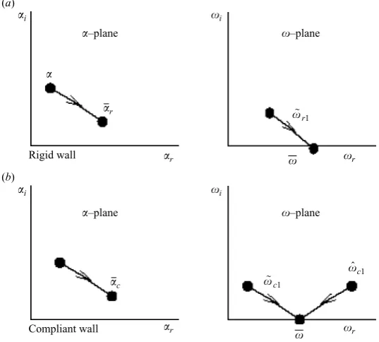
Figure 4.A schematic sketch illustrating the relationship between the eigenstates in the

α-plane and the generalized temporal eigenstates in theω-plane. Subscripts ‘r’ and ‘i’ refer to real and imaginary parts.

The relationship betweenδα andδω, obtained from (4.22), gives us the pseudo group velocitycp, the expression for which is given below:

cp = δω δα =−

1

0 ¯θ Lα(¯α,ω¯) ¯φdy 1

0 θ L¯ ω(¯α,ω¯) ¯φdy

. (4.23)

Finally, the equation for the jump λc for the present case, i.e. Route B, is given similarly as in (4.12c) as follows:

λc=−

cgr cp

Ic Ir

, (4.24)

wherecp has been put in place of cgc.

Incidentally, for the rigid-wall case,cp andcg are the same; but for the compliant-wall case these are different. The pseudo group velocity is a new concept, the physical ramifications of which will be described in the next two subsections.

The two routes by which the singular solution is approached for the compliant-wall cases as α → α¯c, viz. ˜ωc1 → ω¯ for Route A and ˆωc1 → ω¯ for Route B, are shown

in figure 4(b). Figure 4(a)shows how the singular solution is approached for the rigid-wall case as α → α¯r, and that ˜ωr1 → ω¯. The route for the rigid-wall case is

unique becausecg=cp.