http://wrap.warwick.ac.uk/
Original citation:
Pennycook, Simon J., Mudalige, Gihan R., Hammond, Simon D. and Jarvis, Stephen A.,
1970- (2010) Parallelising wavefront applications on general-purpose GPU devices. In:
26th UK Performance Engineering Workshop (UKPEW10), University of Warwick,
Coventry, UK, 8-9 July 2010. Published in: Proceedings of the 26th UK Performance
Engineering Workshop (UKPEW 2010) pp. 111-118.
Permanent WRAP url:
http://wrap.warwick.ac.uk/47468
Copyright and reuse:
The Warwick Research Archive Portal (WRAP) makes this work by researchers of the
University of Warwick available open access under the following conditions. Copyright ©
and all moral rights to the version of the paper presented here belong to the individual
author(s) and/or other copyright owners. To the extent reasonable and practicable the
material made available in WRAP has been checked for eligibility before being made
available.
Copies of full items can be used for personal research or study, educational, or
not-for-profit purposes without prior permission or charge. Provided that the authors, title and
full bibliographic details are credited, a hyperlink and/or URL is given for the original
metadata page and the content is not changed in any way.
A note on versions:
The version presented in WRAP is the published version or, version of record, and may
be cited as it appears here.
Parallelising Wavefront Applications on General-Purpose GPU Devices
S.J. Pennycook, G.R. Mudalige, S.D. Hammond, S.A. Jarvis
Department of Computer Science University of Warwick
CV4 7AL
{sjp,g.r.mudalige,sdh,saj}@dcs.warwick.ac.uk
Abstract—Pipelined wavefront applications form a large portion of the high performance scientific computing workloads at supercomputing centres such as LANL in the United States and AWE in the United Kingdom. This paper investigates the viability of utilising graphics processing units (GPUs) for the acceleration of these codes, using NVIDIA’s Compute Unified Device Architecture (CUDA). Wavefront applications differ from the massively data-parallel codes typically selected for execution on GPUs in that their computation must obey a strict data dependency, limiting the achievable level of parallelism. In this work, we identify a number of optimisations suitable for wavefront codes ported to this new architecture and attempt to quantify the characteristics of those codes that are most likely to experience speedups.
Keywords-CUDA; GPU Computing; Wavefront; Hyperplane
I. INTRODUCTION
The high performance computing (HPC) community is cur-rently experiencing an increased interest in the utilisation of massively data parallel architectures. Graphics process-ing units (GPUs), in particular, have attracted significant attention as an alternative low-cost commodity platform for general-purpose HPC work that would traditionally be run on multi-core processors. With the introduction of program-ming models such as NVIDIA’s Compute Unified Device Architecture (CUDA) [1] and the Open Compute Language (OpenCL) [3], GPU devices are emerging as a viable al-ternative for the acceleration of select HPC applications. Given the potential of GPU accelerated platforms but the apparent complexities associated with the porting of codes,
significant interest remains in understanding theachievable
performance of full applications, not only at individual device level but also multi-node scale.
The research presented in this paper investigates the utilisation of general-purpose GPUs for improving the per-formance of pipelined wavefront applications, which form a large portion of the HPC workloads at supercomputing centres such as the Los Alamos National Laboratory (LANL) in the United States and the Atomic Weapons Establishment (AWE) in the United Kingdom. This class of application differs from general data-parallel problems in that there are significant dependencies between grid-points, which limits achievable level of parallelism from the outset.
A range of different implementations of Lamport’s orig-inal parallel pipelined wavefront “hyperplane” algorithm [9] now exist for a multitude of application domains (e.g. NAS-LU [7], ASCI Sweep3D [4], AWE Chimaera [13] and Smith-Waterman [19]). Considerable effort continues to be spent on the selection of suitable HPC architectures to ensure performant execution of these codes, as witnessed by the continued development and application of high fidelity performance models.
The purpose of this study is to identify which wavefront codes are suitable to be ported to general-purpose GPU
computing. Using an implementation of ageneralwavefront
code on the GPU, we illustrate the potential benefits of a number of optimisations. In so doing, we identify the charac-teristics of wavefront codes which make them amenable for porting. Specifically, we make the following contributions:
• We present an incremental strategy for accelerating
general pipelined wavefront applications on modern high-end GPU hardware. The work utilises a gener-alised demonstrator code that is not specific to any application domain, but replicates the behaviour of real-istic wavefront applications. The utility of this approach allows us to arbitrarily scale the problem size and complexity, permitting flexible exploration of a range of realistic memory access patterns.
• The GPU accelerated code is compared to an equivalent
CPU implementation running on an efficient HPC-capable multi-core processor. We present the runtime of the code for different numbers of processor cores com-municating via the Message Passing Interface (MPI).
• The different behaviours of a range of realistic
wave-front codes are simulated by means of the demonstrator code. These results are used to determine the key char-acteristics of a given wavefront code that can benefit from GPU acceleration.
CPU implementation; and Section VI offers conclusions and suggestions for future work.
II. RELATEDWORK
There have been several previous attempts to accelerate wavefront codes using data-parallel architectures.
In [16], the IBM Cell Broadband Engine (Cell/BE) is utilised to accelerate the Sweep3D benchmark code. The benchmark is migrated to the Cell/BE exploiting five levels of parallelisation: MPI level (which is already implemented on the original benchmark), thread-level, data-streaming level, vector and pipelining. The performance benefits of implementing each of these parallelisation levels are shown in order, demonstrating a path to porting the Sweep3D code to the target architecture. Additionally, a further set of fine-tuning operations are carried out that specifically target the Cell architecture. The Cell/BE implementation is shown to be approximately 4.5 and 5.5 times faster than Sweep3D on a 1.9GHz POWER 5 processor and a 2.6 GHz AMD Opteron processor respectively. It is not made clear how many cores the Opteron processor has, nor whether the Cell/BE’s performance is compared against a single processor core, or multiple cores utilising MPI.
Similarly, [6] presents a parallelisation of a two-dimensional wavefront code – the Smith-Waterman string-matching algorithm – on the Cell/BE. Linear speedup is shown, comparing a single dedicated dual-processor Cell/BE
blade to a serial implementation running on 2.8GHz
dual-core Intel processor. This implementation of the Smith-Waterman algorithm is used to evaluate a performance model for general tiled wavefronts running on the Cell/BE.
In [5], the Smith-Waterman algorithm is implemented on an NVIDIA GeForce GTX 280 using CUDA. The optimi-sation process is described stage-by-stage, identifying four important techniques: the mapping of a one-dimensional thread-block to two-dimensional tiles, coalescence of mem-ory accesses, tiled wavefronts and inter-block synchroni-sation. The issue of inter-block synchronisation is further explored in [20]. The authors report a 9x speedup over a
serial implementation running on a 2.2GHz Intel Core 2 Duo E4500.
Another CUDA implementation of the Smith-Waterman algorithm [11], making use of an NVIDIA GeForce 8800 GTX, reports a 2x to 30x speedup compared to several previous implementations: a traditional implementation run-ning on a 3GHz Pentium 4 processor and an implementation running on the same GPU using OpenGL.
With the exception of [6], these works differ from our own because they are concerned with the acceleration of one wavefront application in particular, rather than the class of wavefront applications in general. Though [6] presents a performance model for general tiled wavefronts, it is not ap-plicable to GPUs and concerned only with two-dimensional wavefronts. Additionally, none of these works demonstrate
t o p = ( i , j , k−1) n o r t h = ( i , j−1 , k ) w e s t = ( i−1 , j , k )
r e s u l t = ( i , j , k )
r e s u l t = fmod ( r e s u l t + t o p + n o r t h + w e s t , c )
Listing 1:Computation per grid-point in the demonstrator wavefront code.
the porting of a three-dimensional wavefront code to the GPU, yet the majority of high-complexity scientific codes operate on three-dimensional data grids. Three-dimensional wavefronts present a challenge because, though they provide
the opportunity of more parallelism, they occupy O(N3)
memory rather than O(N2) which in turn may require
different optimisation strategies or present difficulties in the memory limited context of a GPU. Finally, this work compares a GPU implementation to a parallel multi-core solution, providing a more accurate representation of per-formance than many previous studies. From the outset, this paper compares the potential performance of two devices, not just a full GPU device to a single CPU core. We note that, traditionally, GPU-based porting studies rarely compare against multiple cores, which is how many HPC users will in fact make the comparison.
III. WAVEFRONTAPPLICATIONS ON THEGPU
Typical three-dimensional implementations of the parallel
wavefront algorithm operate over a grid ofNx×Ny×Nz
grid-points. Computation starts at one of the grid’s vertices and progresses to the opposite. By way of example, we
consider a sweep through the data-grid from (0,0,0) to
(Nx −1, Ny −1, Nz −1), in which the computation
re-quired by each grid-point (i, j, k) is dependent upon the
values of three neighbours: (i−1, j, k), (i, j−1, k) and
(i, j, k−1). In [9], Lamport showed that, for a given value
of f, all grid-points that lie on the hyperplane defined by
i+j+k = f can be computed in parallel. Furthermore,
all of the grid-points upon which this computation depends
satisfyi+j+k=f −1; by stepping in f and computing
all satisfied grid-points, the dependency is preserved. To investigate the wavefront algorithm without being specific to any application domain, we have developed a generalised wavefront demonstrator code that replicates the behaviour of a realistic wavefront application. The demon-strator code is capable of performing three-dimensional
sweeps through data grids of sizeN×N×N, where it is
CPU GPU Model Intel Xeon X5550 Tesla C1060
PEs 4 x86 64 Cores 30 SMs
SMT enabled 240 SPs
Clock Rate 2.66GHz/Core 1.3GHz/SP
Memory 12GB RAM 4GB DRAM
Runtime 64-bit Debian CUDA v3.0
[image:4.612.57.295.69.172.2]Environment gcc 4.3.2 Driver 195.36.15
Table I:Experimental setup.
Listing 1 details the computation performed for each grid-point – the wavefront results from the dependency upon the grid-points above, to the north and to the west.
Given the availability of an infinite number of processing elements (PEs), an implementation of the algorithm would assign one grid point per PE and solve the hyperplane
de-fined byi+j+k=fforf = 0...Nx+Ny+Nz−3. However,
realistic data parallel systems will have limited resources, such as the number of available PEs and available memory per device. Thus, decomposing the problem into manageable chunks of work is necessary if any GPU implementation is to scale up to many processor cores, allowing the solution of an arbitrarily large problem size.
A. CUDA Programming Model
In this paper, we implement the wavefront algorithm using the NVIDIA CUDA programming model [1] on a CUDA-capable GPU. The CUDA programming model is, at the time of this research, the most mature programming model compared to its alternatives. There are a wider range of programming and debugging tools available and a CUDA program is more likely to better represent the peak per-formance of an NVIDIA GPU than one written with a third-party API. However, due to the similarities between CUDA and OpenCL, it should be noted that the optimisation strategy detailed here is applicable to all GPUs based upon the CUDA architecture, irrespective of which is used for development.
A CUDA-capable GPU is a collection of relatively low-powered stream multiprocessors (SMs), each consisting of a number of stream processors (SPs) that share control logic and an instruction cache [18]. The amount of global memory (DRAM) and shared memory (SMem) available differs by model; as shown in Table I, the Tesla C1060 used in our experiments provides 4GB of DRAM for the entire GPU and 16KB of SMem per SP. All communication between the CPU and GPU is carried out across a 16x PCI Express (PCIe) 2.0 bus, which has a theoretical bandwidth of 8GB/s. It should also be noted that the Tesla C1060 is optimised for single precision floating-point operations. Though it supports double precision, the difference in performance be-tween single and double precision is known to be significant,
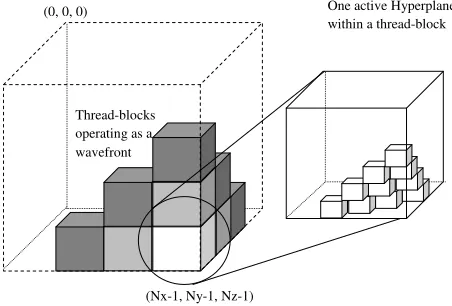
(0, 0, 0)
(Nx-1, Ny-1, Nz-1)
One active Hyperplane within a thread-block
[image:4.612.322.548.72.225.2]Thread-blocks operating as a wavefront
Figure 1:A three-dimensional wavefront operating at two levels of parallelism.
with NVIDIA quoting peak performance figures of 933 and 78 GFLOP/s respectively [2]. As we are interested in the suitability of the GPU architecture for general wavefront codes, both single and double precision performance is discussed in Section V. However, for the sake of simplicity, Section IV lists results from single precision runs exclu-sively.
GPU functions in the CUDA programming model are
written as kernels which, when launched, are executed
simultaneously in a single-instruction-multiple-data (SIMD) fashion by a large number of threads. These threads are
arranged into one-, two- or three-dimensional blocks, with
blocks forming a one- or two-dimensional grid. Thus the
programming model allows for parallelism at two levels – the thread-blocks are assigned to SMs and executed in parallel, whilst the threads themselves are scheduled for
execution in groups of 32 known as warps.
B. A Na¨ıve Port
In order to implement the hyperplane algorithm using the CUDA programing model, we decompose the parallelisation in such a way that we benefit from both levels of parallelism. Figure 1 shows a three-dimensional wavefront mapping when executed under the CUDA programming model.
At the first level, the total problem grid is decomposed into coarse sub-grids, solved via a coarse wavefront op-eration over thread-blocks. The thread-blocks coloured in Figure 1 represent the last three wavefront steps of a
sweep starting at cell (0,0,0) and progressing towards
(Nx−1, Ny−1, Nz−1)– the least recent step is dark grey,
0 0.5 1 1.5 2 2.5 3 3.5
0 5e+07 1e+08 1.5e+08 2e+08 2.5e+08 3e+08
Ex
ecution
T
ime
(in
Seconds)
Number of Grid-Points CPU (1-Core)
[image:5.612.389.485.69.233.2]GPU (Naive) CPU (4-Core)
Figure 2:Graph of execution times for the na¨ıve GPU and CPU implementations operating in single precision.
function for block synchronisation, we implement it through multiple kernel calls. For each wavefront step, a different kernel is launched and only those thread-blocks lying on the wavefront are scheduled for execution.
At the second level, each thread-block is solved by threads operating in a wavefront over the local grid-points assigned to each subgrid. In this na¨ıve implementation, there is a one-to-one mapping from threads to grid-points – each thread in a thread-block is responsible for computing the value of a single grid-point and therefore active in only one wavefront step. The amount of parallelism at this level is further limited by the resources allocated to a thread-block by a GPU; for devices of compute capability 1.3 and below, each
thread-block can contain a maximum of512 threads. Parallelising
at both levels is necessary to overcome this limitation and allow the solution of arbitrarily large problem sizes.
IV. OPTIMISATIONS
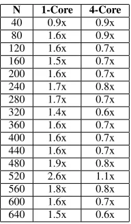
Figure 2 compares the performance of the na¨ıve GPU implementation described in Section III-B to that of single-and quad-core CPU implementations utilising MPI. The execution times shown include the overheads of message passing via MPI for multi-core CPU implementations and of moving data to and from the device via the PCIe bus for the GPU implementation. It should also be noted that due to the difficulty of predicting the effect of a change in block size upon execution time, the fastest times were selected from experiments repeated across all valid launch configurations.
At small problem sizes the speedup is negligible, as the amount of computation is not sufficient to hide the overheads of communication via the PCIe bus and kernel invocation. The speedup figure is more impressive for larger problem
sizes, such as 320×320×320, and we list speedups for
several different values ofN in Table II to account for this.
Though the GPU implementation of the demonstrator code is consistently between 1.5x to 2x faster than the
N 1-Core 4-Core
40 0.9x 0.9x 80 1.6x 0.9x 120 1.6x 0.7x 160 1.5x 0.7x 200 1.6x 0.7x 240 1.7x 0.8x 280 1.7x 0.7x 320 1.4x 0.6x 360 1.6x 0.7x 400 1.6x 0.7x 440 1.6x 0.7x 480 1.9x 0.8x 520 2.6x 1.1x 560 1.8x 0.8x 600 1.6x 0.7x 640 1.5x 0.6x
Table II: Speedup of the na¨ıve GPU implementation, corresponding to the results in Figure 2.
equivalent CPU implementation on a single core, it is approximately 2x slower than a quad-core implementation, even at large problem sizes. Furthermore, there are some problem sizes for which execution time is up to 2.7x times
slower than four CPU cores, typically those for whichN is
a power of two. This slowdown is caused by an inefficient
memory layout, which results in partition camping [17].
Partition camping occurs when some of the threads of a
givenhalf-warpattempt to access memory locations within
the samepartitionof global memory. In these situations, all
such memory requests will be serialised, resulting in poor performance.
It is clear that the performance of the na¨ıve port is sub-optimal. In the following sections, we describe three targeted optimisations designed to decrease execution time and smooth the spikes in performance. Previous works [11], [10] have shown that thread recycling, data rearrangement for coalesced memory accesses and utilisation of shared memory are applicable to two-dimensional wavefront codes; we demonstrate how they can be adapted to a general three-dimensional case.
A. Thread Recycling
The maximum thread-block size permitted under the
one-to-one mapping used by the na¨ıve port is8×8×8, owing to the
limit of 512 threads per SM. This mapping is significantly inefficient; even at the sweep’s most active wavefront step, less than 10% of the threads in the block will be carrying out any computation.
In order to increase efficiency, it is necessary to recycle
[image:5.612.60.291.71.226.2]0 0.5 1 1.5 2 2.5 3 3.5
0 5e+07 1e+08 1.5e+08 2e+08 2.5e+08 3e+08
Ex
ecution
T
ime
(in
Seconds)
Number of Grid-Points GPU (Naive)
[image:6.612.315.566.69.233.2]GPU (Thread Recycling) GPU (Data Rearrangement) GPU (Shared Memory)
Figure 3:Graph of execution times for GPU implementation at different stages of the optimisation
process, operating in single precision.
𝑇6
𝑇6
𝑇6
𝑇7
𝑇7
𝑇6
𝑇8
𝑇7
𝑇6
𝑇3
𝑇3
𝑇3
𝑇1
𝑇4
𝑇3
𝑇5
𝑇4
𝑇3
𝑇0
𝑇0
𝑇0
𝑇1
𝑇1
𝑇0
𝑇2
𝑇1
[image:6.612.60.291.70.227.2]𝑇0
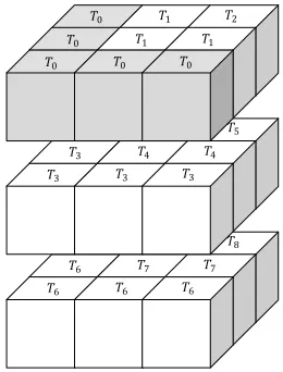
Figure 4: A mapping of threads to a three-dimensional sub-grid.
a block should be equal to the number of grid-points on the largest hyperplane. However, such a complicated mapping is difficult to implement (with support for variable block sizes) without utilising a lookup table stored in global or constant memory.
We have instead opted for a less complicated but sub-optimal thread mapping. In this mapping, as demonstrated
for a3×3×3sub-grid by Figure 4,Nthreads are responsible
for the computation at any given level of the sub-grid. Consider the threads that map to the first of these levels,
namely threads T0, T1 and T2 – T0 is active at every step
and computes the values of the grid-points shaded in grey,
whilst threads T1 and T2 become active only for steps that
update enough grid-points to warrant their execution. This system essentially models the hyperplane as a series of two-dimensional wavefronts operating in parallel, each one step behind that of the previous level. The mapping
N Thread Recycling Data Rearrangement Shared Memory
40 1.1x 0.7x 0.9x
80 1.3x 1.2x 1.4x
120 1.3x 1.7x 2.1x
160 1.2x 2.1x 2.5x
200 1.1x 1.9x 2.4x
240 1.2x 1.9x 2.3x
280 1.1x 2.0x 2.5x
320 1.2x 2.4x 3.0x
360 1.1x 2.1x 2.5x
400 1.2x 2.3x 2.7x
440 1.1x 2.3x 2.8x
480 1.1x 1.9x 2.2x
520 1.3x 1.4x 1.6x
560 1.1x 2.1x 2.5x
600 1.2x 2.2x 2.7x
640 1.6x 2.5x 3.0x
[image:6.612.110.240.286.457.2]Table III: Cumulative speedup yielded by each stage of the GPU optimisation, corresponding to the results in
Figure 3.
of threads to each of these two-dimensional wavefronts is optimal, as the number of threads at each level is equal to the number of grid-points on a level’s leading diagonal. However, in a three-dimensional wavefront, these leading diagonals are never computed simultaneously; there is no wavefront step in which all threads of a block will be active. The resulting decrease in the number of threads (from
N3 to N2) sufficiently demonstrates the effects of thread
recycling upon execution time. As shown by Table III, we see a speedup of between 1.1x and 1.6x over the original na¨ıve GPU implementation. In our experience, it is the
ability to run larger blocks (up to22×22×22) that makes
the most significant difference. By way of example, we see
that solving a16×16×16grid using a single thread-block is
1.8x faster than solving its decomposition into four8×8×8
sub-grids.
For large block sizes, the threads in a single warp still access memory locations in different segments; in the worst case, each memory request will be served by a separate 32-byte transaction. For best performance, memory accesses
should be coalesced according to the coalescence
crite-ria outlined by NVIDIA in [15]. Coalescence of memory accesses requires the rearrangement of the data in global memory.
B. Data Rearrangement
0 0.5 1 1.5 2 2.5 3 3.5
0 5e+07 1e+08 1.5e+08 2e+08 2.5e+08 3e+08
Ex
ecution
T
ime
(in
Seconds)
Number of Grid-Points CPU (1-Core)
[image:7.612.57.293.69.233.2]CPU (4-Core) GPU (Shared Memory)
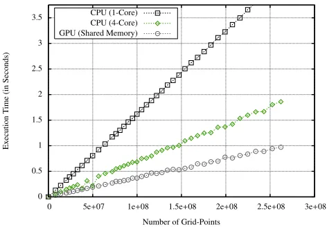
Figure 5:Graph of execution times for the optimised GPU and CPU implementations.
the location of a given grid-point by way of a lookup table stored in constant memory.
However, a rearrangement of this nature is non-trivial. Reading from, and writing to, different data layouts means that one of the two steps cannot be coalesced; the problem of inefficient memory accesses is moved from the
wave-front kernel and into a separatedata rearrangement kernel.
However it is still beneficial for two reasons: firstly, the rearrangement kernels access each memory location only once and secondly, the execution time of the rearrangement kernel is insignificant for large problem sizes.
In addition to this re-ordering of data points, the rear-rangement step introduces two contiguous buffers represent-ing the east and south planes of each sub-grid. The main benefit of this to the demonstrator code is that it becomes simpler to compute the memory locations of a grid-point’s north and west neighbours when it lies upon a thread-block boundary. For wavefront codes operating at scale, these buffers also allow border data to be easily shared across processors using MPI.
Data rearrangement enables each thread’s memory access requests to be served efficiently, leading to a 1.5x speedup over thread recycling and a 1.9x speedup over the na¨ıve implementation. As shown by Figure 2 and Table III, the code also performs much more consistently.
However, each memory location is accessed four times on average – once during its own computation and once by each of the three neighbours whose values depend upon it. This problem is largely an issue with devices of CUDA compute capability below 2.0; NVIDIA’s newest Fermi architecture introduces a caching mechanism that is likely to improve the performance of such codes. For devices without such a cache, it is possible to use the 16KB of shared memory available to each SM for the same purpose.
Single Precision Double Precision N Loops 1-Core 4-Core 1-Core 4-Core
[image:7.612.337.537.70.238.2]40 1 0.8x 0.8x 0.6x 0.4x 80 1 2.2x 1.2x 1.3x 0.8x 160 1 3.8x 1.7x 1.8x 0.8x 320 1 4.3x 1.9x 2.1x 0.9x 640 1 4.4x 1.9x 2.2x 0.9x 40 5 2.5x 0.9x 1.4x 0.7x 80 5 7.5x 2.5x 2.6x 0.9x 160 5 12.9x 3.3x 4.2x 1.4x 320 5 15.6x 4.9x 4.9x 1.6x 640 5 17.2x 5.7x 5.4x 1.8x 40 10 2.9x 1.1x 1.8x 0.7x 80 10 9.1x 3.0x 3.4x 1.1x 160 10 16.9x 5.4x 4.9x 1.6x 320 10 20.1x 6.7x 5.8x 1.8x 640 10 21.3x 7.0x 5.7x 1.8x
Table IV: Speedup of the optimised GPU implementation, operating in both single and double precision.
C. Shared Memory
If one element of shared memory is allocated for each grid-point of sub-grid, then the entire sub-grid and its borders can be pre-fetched with a single contiguous memory access. After a thread-block carries out the computation for its sub-grid, the results can then be transferred back to global memory, again with a single contiguous memory access.
However, this approach requires O(N3) shared memory,
which is large enough to have an adverse affect upon the GPU’s ability to schedule blocks efficiently. For the demon-strator code, the effects of this shared memory overhead are twofold; due to the 16KB memory limit per SM, the maximum thread-block size and the number of thread-blocks running concurrently per SM are both reduced.
An alternative and more flexible approach is to recycle shared memory in a similar way to that of recycling threads, where each thread is assigned three shared memory loca-tions, representing each of the three neighbours from which it must read values. At the end of a given wavefront step, each thread then writes its result into those locations in shared memory that belong to its neighbours.
The utilisation of shared memory leads to a 1.2x speedup over a coalesced thread recycling solution, which yields a combined 2.3x speedup overall. As shown by Table III, this is not as impressive a gain as from the other optimisations, which we believe to be the result of an increase in the number of branching instructions introduced by our shared memory recycling strategy.
V. PERFORMANCERESULTS
Figure 5 and Table IV compare the performance of the fully-optimised GPU implementation of the demonstrator wave-front code with the CPU implementation running on one and
four cores. For the largest problems size (640×640×640)
r e s u l t = ( i , j , k )
f o r ( i = 0 ; i < m a x i t e r a t i o n s ; i ++) {
r e s u l t = fmod ( r e s u l t + t o p + n o r t h + w e s t , c )
t o p = ( t c ∗ t o p ) + t d ; n o r t h = ( nc ∗ n o r t h ) + nd ; w e s t = ( wc ∗ w e s t ) + wd ; r e s u l t = ( r c ∗ r e s u l t ) + r d ;
}
Listing 2:Computation per grid-point in the modified demonstrator code.
double precision, however, we see only a 2.2x and 0.9x speedup – the performance of the GPU is roughly equal to that of the four Nehalem cores.
These speedups are not as high as those that have pre-viously been reported in the literature. It is possible that this is due to the latency of global memory, as the number of floating-point operations performed by the demonstrator code is not high enough to facilitate latency hiding. A sufficient ratio of computation to global memory accesses is required to permit the GPU’s thread scheduler to hide la-tency by executing arithmetic instructions from other warps [14]. The demonstrator code carries out approximately six point operations per grid-point, or three floating-point operations for each memory access, which is not sufficient. It should be noted that these numbers discount setup costs and the extra memory accesses required for border cases; the computation at each grid-point is modelled as one read, one write, three additions and one floating-point modulo operation.
To investigate whether a more realistic wavefront code performing heavier computation would experience more impressive speedups, we increase the per-cell computation in the code by introducing an arbitrarily extensible for loop as
shown in Listing 2. In this modified code,tc,td,nc,nd,
wc,wd,rcandrdare all arbitrary floating-point constants
defined at run-time, preventing the compiler from carrying out any constant-based code optimisations.
An iteration of the loop requires seven additions, four multiplications and one floating-point modulo, which we model as 14 floating-point operations in total. Adjusting the maximum number of iterations allows this number to be in-creased artificially, and Table IV lists the GPU speedup over the CPU implementations for one, five and ten iterations. These iteration counts are equivalent to 7, 35 and 70 floating-point operations per memory access respectively. Though such a large number of floating-point operations may appear unrealistic, it is not an unusual level of computation for scientific codes. For example, ASCI Sweep3D requires 40 floating-point operations per grid-point [8], [12], whilst the NAS-LU benchmark requires approximately 150. The table shows that as the number of loop iterations increases, so too
does the relative speedup. In single precision, the speedup increases to a maximum of 21x for a single core and 7x for four; in double precision, the speedup increases to a maximum of 6x for a single core and 2x for four.
Also of interest is the effect of an increase in the number of loops upon the earlier, unoptimised, GPU implementa-tions. As with the optimised code, the GPU is better able to schedule warps to hide memory latencies; the effects of memory optimisations (discussed in Sections IV-B and IV-C) become less noticeable as global memory loads be-come more efficient. For certain problem sizes and launch configurations, the extra mathematical operations required for index calculations and extra writes to shared memory appear to dominate – a thread recycling solution is up to 1.2x faster than one utilising shared memory.
VI. CONCLUSIONS
This paper has detailed an incremental strategy for the port-ing and acceleration of three-dimensional wavefront codes to general-purpose GPU devices. It has shown that, despite the limited level of parallelism presented by Lamport’s hyperplane method, there is the potential for such codes to experience considerable speedups over traditional serial implementations. However, speedup is less impressive when compared to that of an existing parallel solution utilising MPI, highlighting the necessity of comparing the full po-tential performance at a device to device level.
The performance of the code was examined when using both single and double precision floating-point arithmetic, and the maximum speedup for double precision shown to be reasonable at best. This is significant, as single precision is not sufficient for the majority of scientific codes.
As part of the porting process, we have demonstrated the importance of thread recycling, data rearrangement and the utilisation of shared memory by examining their cumulative effects upon execution time. It is clear that the porting of a three-dimensional wavefront code requires that significant attention be paid to its memory access pattern. In particular, a na¨ıve GPU implementation of such a code is likely to suffer performance degradations not only as a result of inefficient half-warp alignment, but also due to partition camping. The global memory cache introduced in NVIDIA’s new Fermi architecture should go some way to increasing the performance of such unoptimised code ports, however we do not expect such codes to outperform those with data layouts adjusted to target a specific application.
We have also investigated the effects of a change in the amount of computation per grid-point upon speedup. These results conclusively show that wavefront codes with a high ratio of compute to global memory access will be more amenable to porting than other, more memory-intensive codes.
benchmark, such as NAS-LU or Sweep3D. By producing a performance model of its execution, we intend to be able to predict the behaviour of such codes across different CUDA architectures and specific GPU chipsets. These models will also enable us to comment upon the performance of these codes at scale, such as when run in a GPU cluster environ-ment in which nodes communicate via MPI.
REFERENCES
[1] The NVIDIA Compute Unified Device Architecture. http: //www.nvidia.com/cuda/, 2010.
[2] NVIDIA Tesla C1060 Computing Processor - Many Core Supercomputing for Workstations. http://www.nvidia.co.uk/ object/tesla c1060 uk.html, 2010.
[3] OpenCL - The Open Standard for Parallel Programming of Heterogenous Systems. http://www.khronos.org/opencl/, 2010.
[4] The ASCI Sweep3D Benchmark. http://www.llnl.gov/asci benchmarks/asci/limited/sweep3d/asci sweep3d.html, 2010.
[5] A. M. Aji and W. Feng. Accelerating Data-Serial Applications on Data-Parallel GPGPUs: A Systems Approach. Technical Report TR-08-24, Computer Science, Virginia Tech, 2008.
[6] A. M. Aji, W. Feng, F. Blagojevic, and D. S. Nikolopoulos. Cell-SWat: Modeling and Scheduling Wavefront Computa-tions on the Cell Broadband Engine. InCF ’08: Proceedings of the 5th Conference on Computing Frontiers, pages 13–22, New York, NY, USA, 2008. ACM.
[7] D. Bailey, T. Harris, W. Saphir, R. Wijngaart, A. Woo, and M. Yarrow. The NAS Parallel Benchmarks 2.0. Technical Report NAS-95-020, NASA, December 1995.
[8] D.J. Kerbyson, A. Hoisie, and H.J. Wasserman. A Compar-ison Between the Earth Simulator and AlphaServer Systems using Predictive Application Performance Models.Computer Architecture News (ACM), December 2002.
[9] L. Lamport. The Parallel Execution of DO Loops. Commun. ACM, 17(2):83–93, 1974.
[10] Y. Liu, D. Maskell, and B. Schmidt. CUDASW++: Op-timizing Smith-Waterman Sequence Database Searches for CUDA-Enabled Graphics Processing Units. BMC Research Notes, 2(1):73, 2009.
[11] S. Manavski and G. Valle. CUDA Compatible GPU Cards as Efficient Hardware Accelerators for Smith-Waterman Se-quence Alignment. BMC Bioinformatics, 9(Suppl 2):S10, 2008.
[12] G. R. Mudalige, S. A. Jarvis, D. P. Spooner, and G. R. Nudd. Predictive Performance Analysis of a Parallel Pipelined Syn-chronous Wavefront Application for Commodity Processor Cluster Systems. In Proc. IEEE International Conference on Cluster Computing - Cluster2006, Barcelona, September 2006. IEEE Computer Society.
[13] G. R. Mudalige, M. K. Vernon, and S. A. Jarvis. A Plug-and-Play Model for Evaluating Wavefront Computations on Parallel Architectures. In IEEE International Parallel and Distributed Processing Symposium (IPDPS 2008). IEEE Computer Society, April, 2008.
[14] NVIDIA. CUDA Best Practices Guide, Version 3.0. Technical report, NVIDIA Corporation, 2010.
[15] NVIDIA. CUDA Programming Guide Version 3.0. Technical report, NVIDIA Corporation, 2010.
[16] F. Petrini, G. Fossum, J. Fernndez, A. L. Varbanescu, M. Kistler, and M. Perrone. Multicore Surprises: Lessons Learned from Optimizing Sweep3D on the Cell Broadband Engine. In International Parallel and Distributed Process-ing Symposium (IPDPS 2007), pages 1–10. IEEE Computer Society, July 2007.
[17] G. Ruetsch and P. Micikevicius. Optimizing Matrix Transpose in CUDA. Technical report, NVIDIA Corporation, 2009.
[18] S. Ryoo, C. I. Rodrigues, S. S. Baghsorkhi, S. S. Stone, D. B. Kirk, and W. W. Hwu. Optimization Principles and Application Performance Evaluation of a Multithreaded GPU using CUDA. In PPoPP ’08: Proceedings of the 13th ACM SIGPLAN Symposium on Principles and practice of parallel programming, pages 73–82, New York, NY, USA, 2008. ACM.
[19] T.F. Smith and M.S. Waterman. Identification of Common Molecular Subsequences. Journal of Molecular Biology, 147(1):195–197, 1981.